A Machine Learning Approach to Correlation Development Applied to Fin-Tube Bundle Heat Exchangers


1
Department of Energy and Process Engineering, Norwegian University of Science and Technology, NO-7491 Trondheim, Norway
2
Department of Chemical Engineering, Carnegie Mellon University, Pittsburg, PA 15213, USA
*
Author to whom correspondence should be addressed.
Energies 2018, 11(12), 3450; https://doi.org/10.3390/en11123450
Submission received: 18 October 2018
/
Revised: 20 November 2018
/
Accepted: 6 December 2018
/
Published: 10 December 2018
(This article belongs to the Special Issue Fluid Flow and Heat Transfer)
Abstract
:Heat exchanger designers need reliable thermal-hydraulic correlations to optimize heat exchanger designs. This work combines an adaptive sampling method with a Computational Fluid Dynamics (CFD) simulator to obtain increased accuracy and validity range of heat transfer and pressure drop predictions using a limited number of data points. Correlation efficacy was evaluated based on a steam generator case study. The sensitivity to the design parameters was analyzed in detail. The RMSE (root mean square error) of the developed correlations were reduced, through CFD sampling, from 28% to 15% for pressure drop, and from 33% to 25% heat transfer, compared to regression on experimental data only. The best reference correlations have RMSE values of 43% and 33% on pressure drop and heat transfer, respectively, on an independent validation set. Indeed, a radically different fin-tube geometry was suggested for the case study, compared to results using the Escoa correlations.The developed correlations show good to excellent agreement with trends in the CFD model. The quantitative error of predicted heat transfer and pressure drop coefficients at the case study optimum, however, was as large as those of the Escoa correlations. More data are likely needed to improve accuracy for compact heat exchanger designs further.
Dataset License: CC-BY-SA
1. Introduction
Increased energy efficiency is a key strategy to reduce anthropogenic CO emissions, and often the most economical one in the industrial sector. Many energy intensive industries have already implemented measures such as heat integration and bottoming cycles up to its economic potential. An exception to this rule is the offshore oil and gas sector, where space and weight restrictions put severe limits to the amount of equipment that can be placed on each installation.
Volume and weight optimization of an offshore bottoming cycle is contingent on accurate thermal-hydraulic correlations. This is particularly true for the large and heavy waste heat recovery unit (WHRU), which typically consists of a circular fin-tube bundle. Numerical methods such as Computational Fluid Dynamics (CFD) can be used to predict the performance of such heat exchangers, but direct optimization is usually not feasible due to the large number of design variables and constraints and the computational cost (lead time) of each function evaluation.
Many thermal-hydraulic correlations for fin-tube bundles have been presented in the literature over the last half-century. Typically, correlations are algebraic expressions of non-dimensional groups with model constants fitted to experimental data by regression. The underlying data are derived from the authors’ own published experimental work (e.g., [1]), from proprietary databases (e.g., [2]) or from a collection of several literature sources (e.g., [3]). In the two former cases, correlations tend to have a rather limited (or unknown) range of applicability. In the latter case, the underlying data are inherently scattered due to differences in experimental setups, data reduction methods and tube geometry details. This is particularly true for pressure drop measurements, where uncertainties are larger. Earlier work has shown that the WHRU skid weight can be reduced by scaling down the tube diameter to about 10 [4]. This requires new correlations with an extended validity range, to avoid extrapolation. There may also be a need to verify the accuracy of previously published work in a consistent manner.
Machine learning methods represent a contrasting approach to model building, where the model structure is less restricted. Artificial Neural Networks (ANN), Radial Basis function Neural Networks (RBNN) and Support Vector Regression (SVR) models have been used successfully to predict the thermal performance of a number of heat exchanger types. As shown in Table 1, most published studies utilize fully connected ANN models trained on experimental data. More recent publications have also considered other model setups, as well as sampling from a CFD model.
CFD models are increasingly being used for predictive design, even in critical applications such as nuclear reactor thermal-hydraulics [14], provided that rigorous verification and validation practices are adhered to. In the context of fin-tube bundles, CFD models can provide heat transfer and pressure drop coefficients in a consistent and time efficient manner. Comparisons with experimental data has shown good agreement, close to or within the experimental uncertainty, for a wide range of geometries [15]. CFD models are also able to provide data for extreme geometries that may not be possible to manufacture and test experimentally, but still add valuable data in the correlation development process. This includes “adversarial examples”, i.e., geometries where small changes in parameters cause large changes in model output.
Given these developments, we propose to combine predictive CFD simulations with adaptive sampling and automated correlation building methodologies based on machine learning theory. We hypothesize that correlation accuracy and validity range can be increased simultaneously, with reasonable computational effort, by leveraging publicly available experimental work in conjunction with new, adaptively sampled simulation points. This paper provides the underlying simulated data points, in addition to the improved thermal-hydraulic correlations, to foster and accelerate further developments in the field. The presented methodology is applicable to a wide range of multivariate design problems where direct optimization with CFD is infeasible.
Specifically, the novelty of the investigation, as applied to fin-tube thermal-hydraulic correlation development, is the following:
- application of error estimation and adaptive sampling
- direct inclusion of predictive CFD model data in model regression
- extended validity range of geometric parameters towards the weight optimum indicated by earlier work
2. Method
The overall correlation building and verification process used in this article is shown in Figure 1. A design space relevant for waste heat recovery units was firstly defined (see Table 2). An initial database of experimental work from the open literature was fed into the model building software ALAMO version 2018.4.3 [16]. A correlation was generated and improved through adaptive sampling of data points from the CFD simulator. The correlation was then evaluated using a separate validation set, as well as a case study where the optimal point was compared to an independent CFD simulation. The validation set consists of 30 CFD simulations selected through Latin hypercube sampling of the design space, as indicated in Figure 1. Finally, the trends in the different input variables were evaluated using CFD simulations and compared to correlations from the present and earlier work. The remainder of this section describes the components of the methodology in further detail.
2.1. Initial Database
A database of published experimental work has previously been established at the Norwegian University of Science and Technology [17].The database contains data for 248 different fin-tube bundles from 21 publications, including both plain and serrated fin geometries. Several criteria were used to single out and prepare relevant data points for this study:
- Data points outside the ranges defined in Table 2 were omitted. The upper limit on was relatively restrictive since kinematic viscosity for air is about three times higher at 500 compared to usual test conditions (∼ 100 ). Hence, many experimental data points were excluded, but the resulting Reynolds number range (cf. Table 2). was considered representative of the possible operating conditions of a WHRU
- Geometries with only heat transfer or only pressure drop data were removed. A power law function was fitted to the heat transfer data of each remaining geometry and interpolated to the Reynolds numbers at which the (adiabatic) pressure drop was measured. This is necessary because the chosen model building method requires both outputs to be defined at each data point.
- A tube bank array of 30 was considered in this work, as it is the most compact arrangement. Tube banks with array angles in the range 25–35 were corrected using Equation (1), derived from the Escoa correlation [18], to obtain data corresponding to . The maximum applied corrections were 5% for the heat transfer data and 9% for the pressure drop data, respectively. Other tube bank data were discarded.
- The number of streamwise tube rows was not considered as a parameter in this work. Data point duplicates were removed such that only data for the largest number of tube rows were retained.
After this procedure, the remaining database contained 108 experimental data points.
2.2. Correlation Development (ALAMO)
ALAMO is a learning software that identifies simple, accurate surrogate models (correlations) using a minimal set of sample points from black box emulators such as experiments, simulations, and legacy code. ALAMO initially builds a low-complexity surrogate model using a best subset technique that leverages a mixed-integer programming formulation to consider a large number of potential functional forms. The model is subsequently tested, exploited, and improved through the use of derivative-free optimization solvers that adaptively sample new simulation or experimental points. For more information about ALAMO, see Cozad et al. [16,19] and Wilson and Sahinidis [20].
The functional form of a regression model was assumed to be unknown to ALAMO. Instead, several simple basis functions were proposed, e.g., x, , , , and a constant. Once a set of potential basis functions was collected, ALAMO attempted to construct the lowest complexity function that accurately models the initial training data. This model was obtained by minimizing the Bayesian information criterion, , where p is the number of included basis functions, is the sum of squared residuals for the selected model, and is an estimation for the variance of the residuals, which is obtained using the least squares solution of the full basis set or can be specified a priori. The model fitness metric was rigorously minimized using a combination of enumeration, heuristics, and eventual global optimization using the BARON solver [21].
Combinations of linear terms and fractions of the input variables were considered for this particular application, as well as selected powers of these functions with an exponent smaller than unity. Binomial terms, and powers of these, were also considered in modeling the Nusselt number. Once a model was identified, it was improved systematically in ALAMO using an adaptive sampling technique that added new simulation or experimental points to the training set. New sample points were selected to maximize model inconsistency in the original design space, as defined by box constraints on x, using derivative-free optimization methods [22]. It was observed that a higher correlation accuracy was obtained if the outputs and the velocity-related input were log-transformed. It is well known that the velocity dependence is essentially logarithmic and therefore easier to model in log space. As an additional benefit, correlation terms become multiplicative rather than additive. This facilitates interpretation of the correlation as consisting of one velocity-dependent term multiplied with a number of “geometry correction” terms.
2.3. Numerical Model
Numerical simulations in this work followed the methodology described in a previous article [15], where thorough validation with experimental data are given. The main characteristics of the numerical model are as follows:
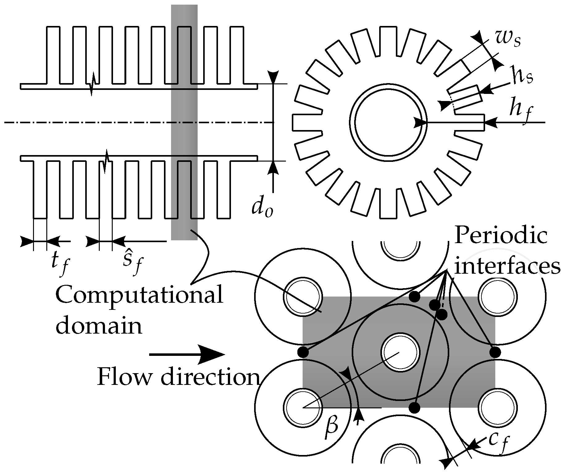
- Fully periodic computational domain (Figure 2) was discretized primarily with hexahedral cells. A graded boundary layer grid was used in the wall normal direction in the space between the fins ().
- Density and thermophysical properties were considered constant, properties for air were used for the external fluid and the fin thermal conductivity was set corresponding to carbon steel ( //).
- The steady-state Reynolds Averaged Navier–Stokes (RANS) equations were solved together with the energy equation and the Spalart–Allmaras turbulence model equation [23] using the open source CFD toolbox OpenFOAM v4.1.
- The Spalart–Allmaras turbulence model was selected due to its simplicity, robustness and suitability for simulating boundary layers under adverse pressure gradient conditions. It also yields similar results as other eddy viscosity turbulence models when applied to finned tube bundles [24]. Model constants were kept at their default value, including the turbulent Prandtl number.
- Second order upwind discretization was used for all convective terms.
- The conjugate heat transfer between the fin and the external fluid was modeled explicitly, resolving the temperature field in the fin. The tube wall thermal resistance was neglected—a uniform temperature was applied at the fin root and on the tube surface. The fluid bulk temperature was specified at the leftmost periodic boundary, avoiding source terms in the energy equation.
- Fin efficiency was evaluated by solving the energy equation a second time, subsequent to RANS model convergence, assuming a frozen flow field and a uniform temperature boundary condition on one fin-tube row. The resulting heat flux was used to compute the fin efficiency in the first simulation having finite thermal conductivity in the fin.
- The computed heat flux, bulk temperature and total pressure drop were normalized into Nusselt and Euler numbers according to standard practice (see, e.g., [17]).
2.4. Accuracy Evaluation
The accuracies of the correlations were evaluated based on the coefficient of determination () and root mean square error (RMSE) values on an independent dataset sampled using CFD (). Some samples struggled to reach iterative convergence during CFD simulation, in which case the flow velocity was reduced. The RMSE is expressed in terms of the deviation from the observed values, viz.
for the predicted values (from correlations) and the observed values (from CFD simulations). Note that the RMSE is equal to the standard deviation for an unbiased estimator.
2.5. Case Study and Verification of Optimal Point
A case study was defined to test the developed correlation on a realistic optimization task and compare the computed optimal point to that obtained using a reference correlation. The predicted heat transfer and pressure drop coefficients were also compared to those predicted by CFD simulations. A boiler section of a generic offshore heat recovery steam generator was considered, with the steam and exhaust gas specifications and constraints given in Table 3. The tube wall temperature was considered constant, and heat conduction through the tube wall, as well as steam/water pressure drop, was neglected. This leads to a computationally cheap heat balance, which can be evaluated using the -NTU method as a function of the exhaust mass flow, cold end temperature difference, and gas side heat transfer coefficient. The objective function is the fin-tube bundle weight, where the tube wall thickness is calculated as
where is the steam pressure and is the yield stress of carbon steel at 500 . The fins were assumed to be made from carbon steel (, ). A theoretical fin efficiency according to Hashizume et al. [25] was used. The ideal gas law was used to evaluate the exhaust gas density at the average bulk temperature, and all other physical properties were considered constant.
The number of tube rows in the transverse and longitudinal directions were modeled as real numbers to obtain a smooth objective function. was calculated directly from the pressure drop constraint, whereas was a free variable. Remaining free variables and bounds were equal to the design variables and bounds in Table 2, with the fin thickness lower bound set to and adjusted to give 20 segments per revolution for serrated fins. A tube bundle layout angle of 30 was used throughout.
The optimization problem was solved in MATLAB R2017a using the built-in function fmincon that implements the SQP algorithm. The optimization was repeated 100 times for a given case, using random starting points within the design space, to ensure that a global, feasible optimum point was reached.
3. Results and Discussion
3.1. Correlation Development
The accuracy evaluation (Table 4) confirmed a relatively good fit between the developed correlations and the independently sampled validation set. The coefficient of determination is high for the Euler number, but less impressive for the Nusselt number. The RMSE is acceptable for the Euler number, but quite large for the Nusselt number, particularly when considering that the 95% confidence interval is much wider than the RMSE.
The difficulty in modeling the Nusselt number may be due to complex changes in the flow field, whereby the flow bypasses the aperture between the fins and flow outside the fin diameter for certain geometric configurations (typically low fin apertures and large fin tip clearances). This phenomenon has been more thoroughly discussed in [27], but ultimately necessitates a different modeling approach than the current one due to the large nonlinearity involved.
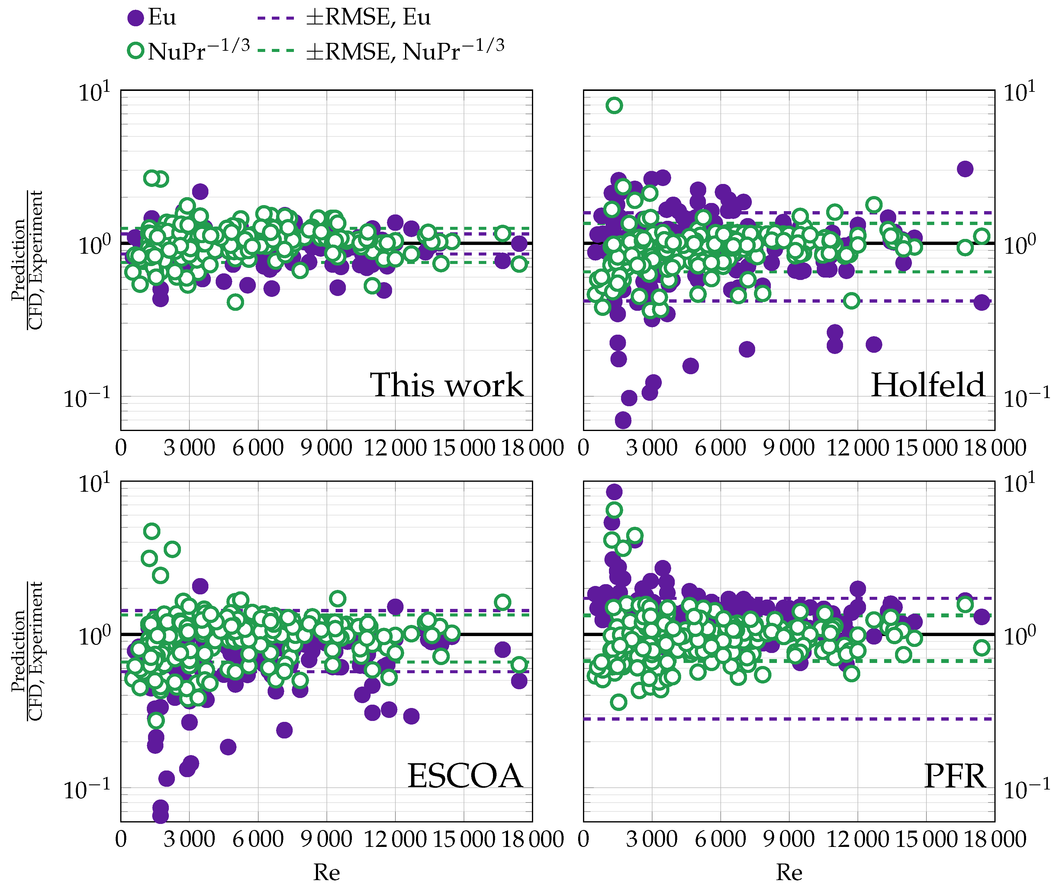
The predictive accuracies for the reference correlations (Holfeld [17], Escoa [18] and PFR [26]) are, in general, poor due to the severe extrapolation induced by the design space definition. As shown in Figure 3, the general scatter for the reference correlations on all data in this work (empirical database, adaptively sampled simulations and simulations used for validation) is large, particularly for low Reynolds numbers. The PFR correlation for Eu has a relatively high coefficient of determination compared to the Escoa and Holfeld correlations, indicating that the hydraulic diameter (which is the unique feature of the PFR Eu correlation) may be a more robust length scale than the tube diameter. The high RMSE associated with the PFR Eu correlation is due to a positive bias (overprediction) that would be simple to rectify with a constant correction factor.
The detailed functional form of the developed correlations is further discussed in Section 3.3. Algebraic expressions of the correlations are provided in the Appendix A.
3.2. Case Study
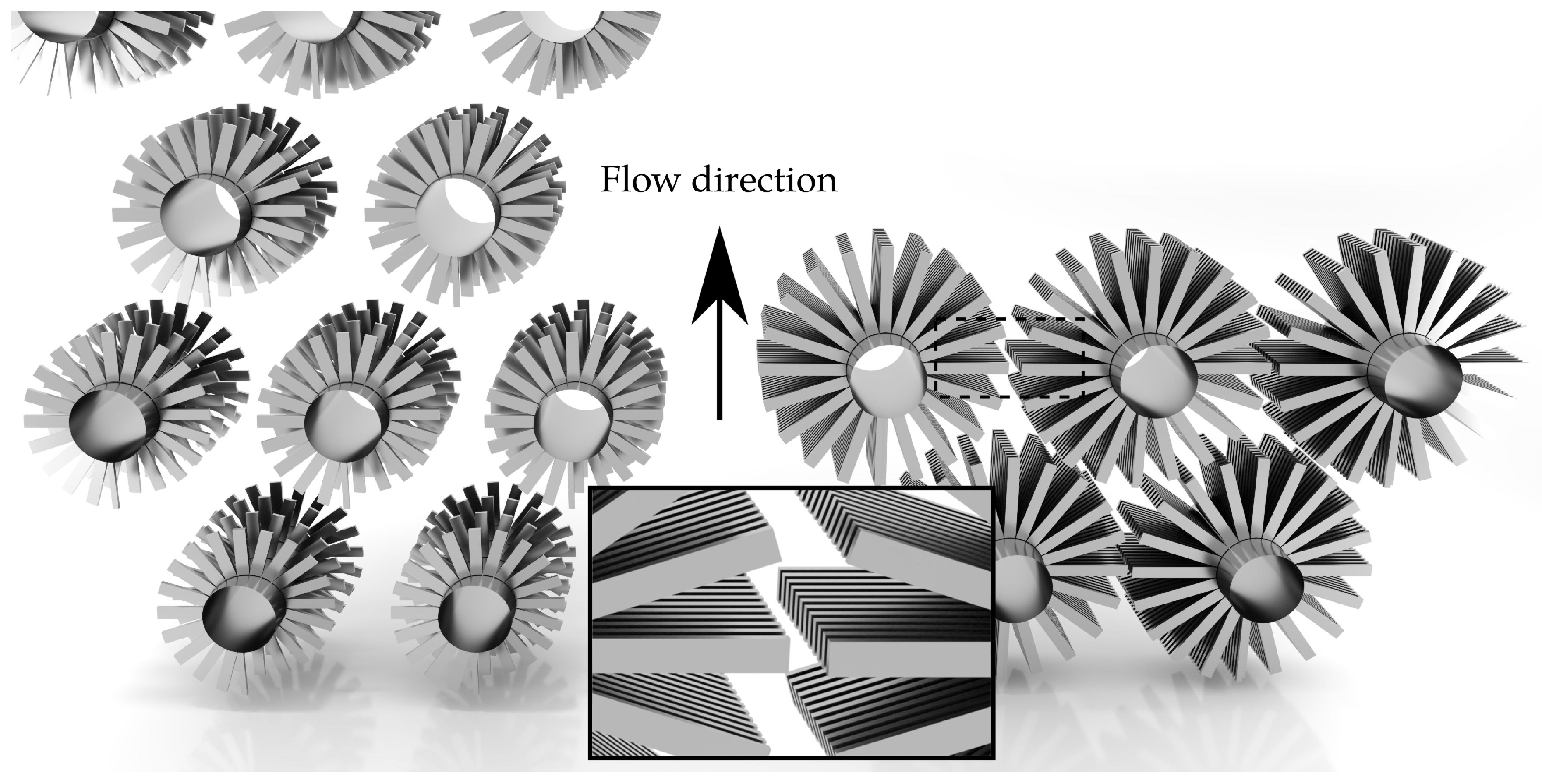
Results from the case study consist of four optimized geometries, two for each correlation with and without an explicit tube diameter constraint, respectively. Geometries and thermal-hydraulic results are given in Table 5 and 3D representations of the two geometries without diameter constraints are shown in Figure 4.
Clearly, two different strategies towards fulfilling the heat duty under a pressure drop constraint emerge for the two different correlations. The optimal geometry for the correlations developed in this work is extremely compact (dense) with a few number of tube rows and a high surface area per tube, but a large frontal area. The optimal geometry using the Escoa correlations, on the other hand, aim to reduce the Euler number such that a larger number of tube rows can be afforded under the pressure drop constraint. This results in a smaller frontal area and a more “open” geometry with less heat transfer area per tube.
Note that the tube diameter reaches its lower bound, and the flow velocity its upper bound, for both correlations. This result is as expected, since the Nusselt number (=) scales with approximately and therefore for a constant velocity. The heat transfer area scales with the perimeter of the tube (disregarding the fins for a moment), leading to . The Euler number (i.e., the pressure drop), on the other hand, scales with at best. This mean that the heat transfer coefficient decreases at the same rate as the pressure drop. A hypothetical doubling of the tube diameter changes the transferred heat by a factor of and the pressure drop by a factor of . If the number of tube rows are increased accordingly (to utilize the available pressure drop), the transferred heat can be increased to and the transferred heat per unit surface area is the same as for the smaller tubes. The weight of the larger tubes, however, is higher than the smaller tubes due to a larger wall thickness and larger internal fluid volume. The only caveat to the argument for a small tube diameter is that restrictions on the steam side pressure drop, steam side heat transfer coefficient, boiling stability and heat exchanger frontal area are not considered here. Moreover, large diameter tubes are less susceptible to flow induced vibrations due to a higher bending stiffness.
Optimization with a fix tube diameter show that similar geometries are obtained as when the tube diameter is free, only with larger frontal area, fewer tube rows and a higher total weight.
The correlation accuracy at the optima, quantified by the deviations from the CFD simulation results, showed mixed performance. The pressure drop was grossly overpredicted by the correlation developed in this work, whereas the heat transfer coefficient was grossly overpredicted by the Escoa correlation. The normalized objective function should therefore be interpreted with care. The optimized geometry using correlations from this work turn out to be conservative (would satisfy heat duty and pressure drop constraints), whereas the optimized Escoa geometries would transfer too little heat.
However, the trends in the prediction of the design variables may be just as important as the accuracy at the optimum, since these trends determine the location of the optimum to begin with. This is the topic of the sensitivity analysis.
3.3. Sensitivity Analysis
The trends in Eu and Nu with respect to the flow velocity and the five geometric variables are shown, for perturbations around the midpoint of the design space, in Figure 5 and Figure 6. These figures also include independent CFD simulations (not included in the training data) at the optimum and at perturbations around the optimum (with remaining variables held constant). Corresponding figures for perturbations around the optimal point in the case study are Figure 7 and Figure 8.
The Euler number exhibits a high sensitivity to the flow velocity and the fin aperture compared to the other four variables (Figure 5 and Figure 7). The velocity dependence can be explained as a transition from friction dominated drag to a mix of friction and form drag as velocity increases. At the design space midpoint, both of these pressure losses seem to be of equal importance, since the sensitivity to increases in wake size () and increases in friction area () is about the same. At the optimum point, a higher sensitivity to the wake size relative to friction area can be noticed (Figure 7, top middle and top right panels) due to the higher flow velocity.
The sensitivity to the fin aperture at constant mean flow velocity should be interpreted in light of the small fin pitches used in this work. Not only does a smaller fin aperture mean more friction area per unit tube length, but also corresponds to a higher maximum flow velocity between the fins required to maintain the same mean velocity. In other words, the blockage caused by the boundary layers on the fins is significant compared to the available cross-sectional (flow) area for the considered range of fin apertures. The lack of a positive correlation between the Euler number and the degree of serration () is unexpected, given that serrations break up the fin boundary layer and hence decrease the average boundary layer thickness. On the other hand, the correlation between and the Nusselt number is also small and, therefore, consistent with the Euler number results. These observations point towards a conclusion that the thermal-hydraulic benefit of serrated fins lie primarily in the increased fin efficiency.
The Nusselt number is primarily a function of the flow velocity and the tube diameter (Figure 6 and Figure 8). Considering that , i.e., linear in , the heat transfer coefficient is approximately constant with the tube diameter as well as with the other geometric parameters. This can be expected in this case, since the heat transfer resistance consists of external boundary layers.
A trend change in can be noted when comparing sensitivities at the midpoint and the optimal point (lower middle panels, Figure 6 and Figure 8): The Nusselt number is relatively constant at the midpoint, but shows a clear negative trend at the optimal point. A possible explanation involves the already mentioned bypass effect. At the midpoint, a decrease in increases the pressure drop (Figure 5), but also redistributes the flow to the passage outside the fin perimeter. The increased pressure drop does not translate to an increased heat transfer coefficient (Figure 6). A small fin tip gap on the other hand, such as at the optimal point, suppresses the bypass effect and forces the flow to pass through the fin aperture. Hence, a decrease in does translate into both increased pressure drop and heat transfer coefficient. The effect is further discussed in [27].
The reference correlations exhibit the correct variable trend in most cases. The PFR correlations captures the trend around the optimal point to a surprising degree, given its simplicity. The quantitative accuracy of the reference correlations, however, is not satisfactory at the optimal point. The Holfeld correlations, which are the most recently developed, grossly underpredict the pressure drop and show incorrect trends for Eu as a function of and Nu as a function of .
The correlations developed in this work generally agree well with the CFD simulations. Trends in and are exaggerated at the case study optimum, most likely due to limited amount of data in the design space, but generally provides improved prediction accuracy.
4. Conclusions
Machine learning methods, including adaptive sampling using a CFD simulator, has been used to improve the accuracy and validity range of thermal-hydraulic correlations for fin-tube bundles, in terms of both the coefficient of determination () and the root mean square error. The applicability to geometry optimization was verified through a case study and the accuracy of the modeling of trends in the design space was confirmed by comparison with CFD simulations. The following specific conclusions can be drawn:
- The choice of correlation is decisive for the outcome of tube bundle weight optimization, at least for the boiler section considered in the case study. The developed correlations suggest a radically different design compared to the Escoa correlations.
- The trends of the developed correlations generally match well with data from the CFD model. The sensitivity to the design variables close to the optimal point for the case study is, however, exaggerated for some variables.
- The PFR correlation for the Euler number is the most robust reference correlation with regards to the trends in the design variables, indicating that the hydraulic diameter can be an appropriate length scale for pressure drop modeling.
- The Nusselt number is relatively insensitive to all design parameters other than the flow velocity and the tube diameter (i.e., the Reynolds number) around the studied design points.
- In general, the Nusselt number appears more difficult to model accurately, compared to the Euler number. A possible explanation, given the preceding bullet point, is that particular geometries cause complex flow redistribution that only a highly nonlinear model can represent.
- Quantitative accuracy on the case study is good for the developed heat transfer correlation, but disappointing for the pressure drop correlation. The accuracy of the Escoa correlations is also poor at the case study optimum. More data are most likely needed in the range of compact designs with low tube diameter, if further accuracy improvements are to be achieved.
The machine learning approach appears to be a viable method to extend the validity range of thermal-hydraulic correlations, with relatively moderate resource usage. As ever, the dataset size limits the model nonlinearity that can be used without overfitting to the training data. Further increase in accuracy will, most likely, require significantly larger datasets created by a combination of structured sampling methods (e.g., Latin hypercube) and adaptive sampling methods.
A limitation of the current study is that the correlation accuracy is restricted to the accuracy of the numerical model. The numerical model is successfully validated over a large range of geometric parameters for which experimental data exist [15]; Future directions of this work should therefore include experimental investigations of previously untested geometries indicated by the correlations, such as at the case study optimum indicated in this work.
Supplementary Materials
The following are available online at https://www.mdpi.com/1996-1073/11/12/3450/s1, Table S1: Underlying CFD simulation data: regression data points, Table S2: Underlying CFD simulation data: validation data points.
Author Contributions
Conceptualization, K.L., E.N. and N.V.S.; Methodology, Z.W., N.V.S. and K.L.; Software, Z.W. and N.V.S.; Formal analysis, K.L. and Z.W.; Investigation, K.L. and Z.W.; Data curation, K.L. and E.N.; Writing—original draft preparation, K.L. and Z.W.; Writing—review and editing, N.V.S. and E.N.; Visualization, K.L.; and Supervision, N.V.S. and E.N.
Funding
K.L. and E.N. acknowledge the partners: Neptune Energy Norge AS, Alfa Laval, Equinor, Marine Aluminium, NTNU, SINTEF and the Research Council of Norway, strategic Norwegian research program PETROMAKS2 (#233947) for their support KL further acknowledges the travel support from Hans Mustad og Robert og Ella Wenzins legat ved Norges teknisk- naturvitenskapelige universitet that enabled the visit at Carnegie Mellon University.
Conflicts of Interest
The authors declare no conflict of interest. The funding sponsors has approved the decision to publish the results, but had no role in the design of the study; in the collection, analyses, or interpretation of data or in the writing of the manuscript.
Abbreviations
The following abbreviations are used in this manuscript:
| ALAMO | Automated Learning of Algebraic Models for Optimization |
| ANN | Artificial Neural Network |
| BIC | Bayesian Information Criterion |
| CFD | Computational Fluid Dynamics |
| RANS | Reynolds Average Navier–Stokes |
| RBNN | Radial Basis function Neural Network |
| RMSE | Root Mean Square Error |
| SVR | Support Vector Regression |
| WHRU | Waste Heat Recovery Unit |
Nomenclature
| Roman symbols | |
| fin heat transfer area [] | |
| tube heat transfer area [] | |
| fin tip-to-tip clearance [] | |
| outer tube diameter [] | |
| total fin height [] | |
| segmented height [] | |
| number of streamwise tube rows [-] | |
| number of transverse tube rows [-] | |
| p | total pressure [] |
| transverse tube pitch [] | |
| longitudinal tube pitch [] | |
| fin pitch [] | |
| fin aperture (=) [] | |
| fin thickness [] | |
| tube wall thickness [] | |
| mean velocity in minimum free flow area [] | |
| segment width [] | |
| Greek symbols | |
| outer heat transfer coefficient [] | |
| tube bundle layout angle [] | |
| fin efficiency [-] | |
| thermal conductivity [] | |
| kinematic viscosity [] | |
| modified turbulent viscosity [] | |
| density [] | |
| yield stress [-] | |
| Dimensionless numbers | |
| Reynolds number | |
| Euler number | |
| Nusselt number | |
| Prandtl number | |
Appendix A
Algebraic expressions for the regression models developed in this work are given in Equations (A1) and (A2). All dimensions (, , etc.) must be in millimeters due to the dimensional nature of some of the regression constants.
References
- Ma, Y.; Yuan, Y.; Liu, Y.; Hu, X.; Huang, Y. Experimental investigation of heat transfer and pressure drop in serrated finned tube banks with staggered layouts. Appl. Therm. Eng. 2012, 37, 314–323. [Google Scholar] [CrossRef]
- Weierman, C. Correlations ease the selection of finned tubes. Oil Gas J. 1976, 74, 10–94. [Google Scholar]
- Nir, A. Heat transfer and friction factor correlations for crossflow over staggered finned tube banks. Heat Transf. Eng. 1991, 12, 43–58. [Google Scholar] [CrossRef]
- Skaugen, G.; Walnum, H.T.; Hagen, B.A.L.; Clos, D.P.; Mazzetti, M.; Nekså, P. Design and optimization of waste heat recovery unit using carbon dioxide as cooling fluid. In Proceedings of the ASME 2014 Power Conference, Baltimore, MD, USA, 28–31 July 2014; pp. 1–10. [Google Scholar]
- Pacheco-Vega, A.; Sen, M.; Yang, K.T.; McClain, R.L. Neural network analysis of fin-tube refrigerating heat exchanger with limited experimental data. Int. J. Heat Mass Transf. 2001, 44, 763–770. [Google Scholar] [CrossRef]
- Islamoglu, Y. A new approach for the prediction of the heat transfer rate of the wire-on-tube type heat exchanger - Use of an artificial neural network model. Appl. Therm. Eng. 2003, 23, 243–249. [Google Scholar] [CrossRef]
- Islamoglu, Y.; Kurt, A. Heat transfer analysis using ANNs with experimental data for air flowing in corrugated channels. Int. J. Heat Mass Transf. 2004, 47, 1361–1365. [Google Scholar] [CrossRef]
- Xie, G.N.; Wang, Q.W.; Zeng, M.; Luo, L.Q. Heat transfer analysis for shell-and-tube heat exchangers with experimental data by artificial neural networks approach. Appl. Therm. Eng. 2007, 27, 1096–1104. [Google Scholar] [CrossRef]
- Peng, H.; Ling, X. Predicting thermal-hydraulic performances in compact heat exchangers by support vector regression. Int. J. Heat Mass Transf. 2015, 84, 203–213. [Google Scholar] [CrossRef]
- Hassan, M.; Javad, S.; Amir, Z. Evaluating different types of artificial neural network structures for performance prediction of compact heat exchanger. Neural Comput. Appl. 2017, 28, 3953–3965. [Google Scholar] [CrossRef]
- Thibault, J.; Grandjean, B.P.A. A neural network methodology for heat transfer data analysis. Int. J. Heat Mass Transf. 1991, 34, 2063–2070. [Google Scholar] [CrossRef]
- Koo, G.W.; Lee, S.M.; Kim, K.Y. Shape optimization of inlet part of a printed circuit heat exchanger using surrogate modeling. Appl. Therm. Eng. 2014, 72, 90–96. [Google Scholar] [CrossRef]
- Shi, H.N.; Ma, T.; Chu, W.X.; Wang, Q.W. Optimization of inlet part of a microchannel ceramic heat exchanger using surrogate model coupled with genetic algorithm. Energy Convers. Manag. 2017, 149, 988–996. [Google Scholar] [CrossRef]
- Bauer, R.C. A framework for implementing predictive-CFD capability in a design-by-simulation environment. Nuclear Technol. 2017, 200, 177–188. [Google Scholar] [CrossRef]
- Lindqvist, K.; Næss, E. A validated CFD model of plain and serrated fin-tube bundles. Appl. Therm. Eng. 2018, 143, 72–79. [Google Scholar] [CrossRef]
- Cozad, A.; Sahinidis, N.V.; Miller, D.C. Learning surrogate models for simulation-based optimization. AIChE J. 2014, 60, 2211–2227. [Google Scholar] [CrossRef]
- Holfeld, A. Experimental Investigation of Heat Transfer and Pressure Drop in Compact Waste Heat Recovery Units. Ph.D. Thesis, Norwegian University of Science and Technology, Trondheim, Norway, 2016. [Google Scholar]
- ESCOA Fintube Corp. ESCOA Engineering Manual (Electronic Version). Technical Report. 2002. Available online: http://www.fintubetech.com/escoa/ (accessed on 1 September 2005).
- Cozad, A.; Sahinidis, N.V.; Miller, D.C. A combined first-principles and data-driven approach to model building. Comput. Chem. Eng. 2015, 73, 116–127. [Google Scholar] [CrossRef]
- Wilson, Z.T.; Sahinidis, N.V. The ALAMO approach to machine learning. Comput. Chem. Eng. 2017, 106, 785–795. [Google Scholar] [CrossRef] [Green Version]
- Kılınç, M.; Sahinidis, N.V. Exploiting integrality in the global optimization of mixed-integer nonlinear programming problems in BARON. Optim. Methods Soft. 2019, 33, 540–562. [Google Scholar] [CrossRef]
- Rios, L.M.; Sahinidis, N.V. Derivative-free optimization: A review of algorithms and comparison of software implementations. J. Glob. Optim. 2013, 56, 1247–1293. [Google Scholar] [CrossRef]
- Spalart, P.; Allmaras, S. A one-equation turbulence model for aerodynamic flows. La Reserche Aérospatiale 1994, 1, 5–21. [Google Scholar]
- Nemati, H.; Moghimi, M. Numerical Study of Flow Over Annular-Finned Tube Heat Exchangers by Different Turbulent Models. CFD Lett. 2014, 6, 101–112. [Google Scholar]
- Hashizume, K.; Morikawa, R.; Koyama, T.; Matsue, T. Fin Efficiency of Serrated Fins. Heat Transf. Eng. 2002, 23, 6–14. [Google Scholar] [CrossRef]
- PFR Engineering Systems Inc. Heat Transfer and Pressure Drop Characteristics of Dry Tower Extended Surfaces; Technical Report, PFR Report BNWL-PFR-7-100; PFR Engineering Systems Inc.: Sante Fe Springs, CA, USA, 1976. [Google Scholar]
- Lindqvist, K.; Næss, E. On correction factors in thermal-hydraulic correlations for compact fin-tube bundles. Heat Mass Transf. 2018. submitted. [Google Scholar]
Figure 1.
Process for correlation development, testing and benchmarking. Green boxes indicate where CFD simulations are employed.
Figure 1.
Process for correlation development, testing and benchmarking. Green boxes indicate where CFD simulations are employed.

Figure 2.
Geometric parameters of the fin-tube bundle and CFD computational domain.

Figure 3.
Predictive accuracy on regression and validation data (208 data points): correlations developed in this work (Supplementary Materials) and correlations from Holfeld [17], Escoa [18] and PFR [26].
Figure 3.
Predictive accuracy on regression and validation data (208 data points): correlations developed in this work (Supplementary Materials) and correlations from Holfeld [17], Escoa [18] and PFR [26].

Figure 4.
Optimized boiler geometry using the Escoa correlations (left) and correlations developed in this work (right), without explicit diameter constraints.
Figure 4.
Optimized boiler geometry using the Escoa correlations (left) and correlations developed in this work (right), without explicit diameter constraints.

Figure 5.
Trends in correlations and CFD simulator around the midpoint in the design space (marked by a circle). CFD simulations were independently sampled (not part of the dataset used for model development). Each parameter was varied independently, with remaining parameters held constant.
Figure 5.
Trends in correlations and CFD simulator around the midpoint in the design space (marked by a circle). CFD simulations were independently sampled (not part of the dataset used for model development). Each parameter was varied independently, with remaining parameters held constant.

Figure 6.
Trends in correlations and CFD simulator around the midpoint in the design space (marked by a circle). CFD simulations were independently sampled (not part of the dataset used for model development). Each parameter was varied independently, with remaining parameters held constant.
Figure 6.
Trends in correlations and CFD simulator around the midpoint in the design space (marked by a circle). CFD simulations were independently sampled (not part of the dataset used for model development). Each parameter was varied independently, with remaining parameters held constant.

Figure 7.
Trends in correlations around the case study optimum found using correlations developed in this work (marked by a circle). CFD simulations were independently sampled (not part of the dataset used for model development). Each parameter was varied independently, with remaining parameters held constant at the optimum.

Figure 8.
Trends in correlations around the case study optimum found using correlations developed in this work (marked by a circle). CFD simulations were independently sampled (not part of the dataset used for model development). Each parameter was varied independently, with remaining parameters held constant at the optimum.


Table 1.
Published work on thermal-hydraulic heat exchanger modeling using machine learning methods.
Table 1.
Published work on thermal-hydraulic heat exchanger modeling using machine learning methods.
| Data Source | Experimental | Correlation or CFD |
|---|---|---|
| Fully connected ANN | [5,6,7,8,9,10] | [11] |
| SVR, RBNN, Kriging | [9] | [12,13] |
Table 2.
Considered design space for compact fin-tube bundles. Ancillary variables are adjusted to achieve a reasonable number of segments per fin revolution and a representative fin efficiency. Geometric parameters are shown in Figure 2.
Table 2.
Considered design space for compact fin-tube bundles. Ancillary variables are adjusted to achieve a reasonable number of segments per fin revolution and a representative fin efficiency. Geometric parameters are shown in Figure 2.
| Design Variables | Min | Max |
|---|---|---|
| [m/s@500 C] | 2.53 | 30.4 |
| [mm] | 9.65 | 50.8 |
| [mm] | 1.4 | 25.4 |
| [-] | 0.0 | 1.0 |
| [mm] | 0.49 | 4.9 |
| [mm] | 0.39 | 8.0 |
| Ancillary and Derived Variables | ||
| Re [-] | 310 | 19,000 |
| [mm] | 0.3 | 0.75 |
| [mm] | 2.0 | 4.0 |
| [deg] | 30.0 | 30.0 |
The tube bundle layout angle is defined as .
Table 3.
Boiler section case study: Definitions and constraints.
| Exhaust mass flow [kg/s] | 75.0 |
| Exhaust pressure drop [Pa] | 1500 |
| Steam pressure [Pa] | 25 × 10 |
| Steam/water temperature [C] | 224 |
| Cold end temperature difference [C] | 20 |
| Transferred heat [W] | ≥15× 10 |
| Narrow gap flow velocity [m/s] | ≤30 |
| Frontal cross-section | square |
Table 4.
Accuracy on validation dataset, computed from Latin hypercube sample of design space (30 CFD simulations).
Table 4.
Accuracy on validation dataset, computed from Latin hypercube sample of design space (30 CFD simulations).
| Model | Eu | NuPr | |||
|---|---|---|---|---|---|
| RMSE | RMSE | ||||
| [-] | [%] | [-] | [%] | ||
| This work | |||||
| database only | 0.75 | 28 | 0.70 | 33 | |
| after sampling | 0.94 | 15 | 0.76 | 25 | |
| Holfeld [17] | −0.08 | 58 | 0.75 | 35 | |
| Escoa [18] | −0.05 | 43 | 0.42 | 34 | |
| PFR [26] | 0.79 | 72 | 0.59 | 33 | |
Table 5.
Case study: Geometry optima for correlations from this work and Escoa, without (left column) and with explicit diameter constraint of 25.4 mm (right column). Eu and NuPr data are computed at the closest geometry possible to simulate with CFD.
Table 5.
Case study: Geometry optima for correlations from this work and Escoa, without (left column) and with explicit diameter constraint of 25.4 mm (right column). Eu and NuPr data are computed at the closest geometry possible to simulate with CFD.
| Correlations: | This Work | Escoa | ||
|---|---|---|---|---|
| Geometry | ||||
| Re [-] | 3600 | 9400 | 3600 | 9400 |
| [mm] | 9.65 | 25.4 | 9.65 | 25.4 |
| [mm] | 10.9 | 12.7 | 6.28 | 15.8 |
| [mm] | 1.0 | 1.0 | 0.96 | 1.0 |
| [mm] | 0.50 | 0.50 | 0.50 | 0.50 |
| [mm] | 0.49 | 0.49 | 4.90 | 4.90 |
| [mm] | ||||
| [mm] | 0.39 | 0.39 | 8.00 | 8.00 |
| [-] | 2.2 | 1.2 | 21.8 | 17.1 |
| [-] | 140 | 102 | 105 | 52 |
| Normalized objective function | 1.00 | 1.49 | 0.87 | 2.33 |
| Eu [-] | ||||
| This work | 5.64 | 10.8 | ||
| Escoa | 0.594 | 0.76 | ||
| CFD | 3.81 | 6.28 | 0.52 | 0.75 |
| Deviation [%] | +48 | +72 | +13 | −2.2 |
| NuPr [-] | ||||
| This work | 66.6 | 125.0 | ||
| Escoa | 56.8 | 96.5 | ||
| CFD | 67.7 | 136 | 38.9 | 74.4 |
| Deviation [%] | −1.7 | −8.0 | −46 | +30 |
© 2018 by the authors. Licensee MDPI, Basel, Switzerland. This article is an open access article distributed under the terms and conditions of the Creative Commons Attribution (CC BY) license (http://creativecommons.org/licenses/by/4.0/).
Share and Cite
MDPI and ACS Style
Lindqvist, K.; Wilson, Z.T.; Næss, E.; Sahinidis, N.V. A Machine Learning Approach to Correlation Development Applied to Fin-Tube Bundle Heat Exchangers. Energies 2018, 11, 3450. https://doi.org/10.3390/en11123450
AMA Style
Lindqvist K, Wilson ZT, Næss E, Sahinidis NV. A Machine Learning Approach to Correlation Development Applied to Fin-Tube Bundle Heat Exchangers. Energies. 2018; 11(12):3450. https://doi.org/10.3390/en11123450
Chicago/Turabian StyleLindqvist, Karl, Zachary T. Wilson, Erling Næss, and Nikolaos V. Sahinidis. 2018. "A Machine Learning Approach to Correlation Development Applied to Fin-Tube Bundle Heat Exchangers" Energies 11, no. 12: 3450. https://doi.org/10.3390/en11123450
Note that from the first issue of 2016, this journal uses article numbers instead of page numbers. See further details here.