Economic Multiple Model Predictive Control for HVAC Systems—A Case Study for a Food Manufacturer in Germany

Department for Sustainable Products and Processes (upp), University of Kassel, 34125 Kassel, Germany
*
Author to whom correspondence should be addressed.
Energies 2018, 11(12), 3461; https://doi.org/10.3390/en11123461
Submission received: 31 October 2018
/
Revised: 29 November 2018
/
Accepted: 7 December 2018
/
Published: 11 December 2018
(This article belongs to the Collection Smart Grid)
Abstract
:The following paper describes an economical, multiple model predictive control (EMMPC) for an air conditioning system of a confectionery manufacturer in Germany. The application consists of a packaging hall for chocolate bars, in which a new local conveyor belt air conditioning system is used and thus the temperature and humidity limits in the hall can be significantly extended. The EMMPC calculates the optimum energy or cost humidity and temperature set points in the hall. For this purpose, time-discrete state space models and an economic objective function with which it is possible to react to flexible electricity prices in a cost-optimised manner are created. A possible future electricity price model for Germany with a flexible Renewable Energies levy (EEG levy) was used as a flexible electricity price. The flexibility potential is determined by variable temperature and humidity limits in the hall, which are oriented towards the comfort field for easily working persons, and the building mass. The building mass of the created room model is used as a thermal energy store. Considering the electricity price and weather forecasts as well as an internal, production plan-dependent load forecasts, the model predictive controller directly controls the heating and cooling register and the humidifier of the air conditioning system.
1. Introduction and Problem Description
A constantly increasing scarcity of resources, increasing emissions, and the global warming that has been proven in many scientific studies require differentiated and comprehensive solutions [1,2,3]. In addition to a more efficient use of resources, the conversion of the energy supply system to an increased use of renewable energies is also decisive for achieving these goals, which in turn leads to an increase in balancing fluctuating residual loads in the electricity grid. With regard to the global energy demand, about one-third is caused by the building sector [4], of which about half of the energy demand is accounted for by building heating, ventilation, and air conditioning (HVAC) [5,6]. In view of these circumstances, energy efficiency measures and the use of more flexible energy supply technologies in the building sector and in the field of building air conditioning are substantial solutions.
In the field of building HVAC, high energy saving potentials can be exploited in many ways. Scientific research focuses on measures on the building structure and insulation, different air routing concepts, the further development of the various components of an air conditioning system and, above all, the improvement of control technology [7,8,9,10]. Due to the volatile nature of wind and solar, energy demand requires more flexibility. Hence, energy demand can be adapted to energy supply. It stabilises the energy system through the demand response on the one hand and increases the utilisation rate of renewable energy systems on the other hand [11,12]. Several different energy market designs and economic incentives are discussed in both the scientific literature and the political and regulatory decision-making bodies dealing with flexible pricing models [13,14]. For these economic models, smart controllers are needed which react automatically to e.g., real-time pricing.
By developing and implementing an economical, multiple model predictive control (EMMPC), this flexibility potential is realised in an energy- or cost-optimised manner. Demand response can be fulfilled by integrating future, flexible electricity price models based on electricity supply and demand. For the flexible operation of the air conditioning, the air mass of the hall is used as thermal energy storage. Allowing a range of temperature and humidity specifications is a key requirement [15,16,17]. Especially in industries, these ranges are often not applied due to fixed settings and strict specifications of the product. The flexible and efficient control of full air conditioning systems require the solution of complex tasks. Time-varying internal and external disturbances affect the controlled system. Many processes involve time delays, the system goes through many operating conditions, and the required energy has variable price structures. An efficient control approach is able to consider time-dependent disturbances, map a wide range of operating conditions and process variable price structures.
With regard to the current state of research, this paper applies an advanced EMMPC approach for the flexible operation of air conditioning systems in industrial productions. Hereby, the EMMPC approach combines both, the approach of multiple and economic model predictive control to control and optimise non-linear systems under several constraints. The realisation of the flexible air conditioning is shown for a real case of a packaging hall for chocolate bars. The product has strict temperature and humidity specifications. Therefore, the implementation of a new, local conveyor belt air conditioning system is indispensable to achieve these specifications for the hall [15,17,18].
2. State of Research
Due to the manifold tasks that an air conditioning system must fulfil, the system control is highly complex. Depending on the design and application, the air temperature, humidity, air volume flow, and air mixtures (fresh air/exhaust air ratio) must be adjusted and controlled. Since these variables influence each other, the degree of complexity increases significantly. For these reasons, a combination of different control approaches and sequence circuits, which control the respective sub-components is often necessary to ensure efficient plant operation.
In the field of efficient and flexible building air conditioning, which is the focus of the paper, a large number of scientific studies can be considered. The publication of Nardi et al. (2018) [10] provides a more detailed overview of the quantification of heat losses via the building envelope.
The publication of Afram and Janabi-Sharifi (2014) [19] gives a good overview of the control approaches used or under development for air conditioning systems. A distinction is made between “classic control”, “hard control”, “soft control”, and “hybrid control” for air conditioning systems as well as further approaches that cannot be assigned to these categories. The classic control corresponds to the state of the art and is widely and practically applied. The classic control methods for HVAC systems include two-point controllers (on/off), proportional (P), proportional integral (PI), and proportional integral differential (PID) controllers. The so-called “hard control” for air conditioning systems include gain scheduling, optimum control, robust control, model predictive control (MPC), and nonlinear and adaptive control. MPC uses previously created models of the system to be controlled to predict and optimise future system behaviour under changing boundary conditions. Such controllers are used both as a replacement for classic controllers and to perform higher-level control tasks.
So-called fuzzy controllers or the use of artificial neural networks are summarised under the term “soft” or “soft control”. These comparatively new methods for controlling HVAC systems can replace both higher-level and local controllers and perform a wide range of tasks. Fuzzy controllers are based on if-then-else instructions and require a sufficiently deep understanding of the system to be controlled. Artificial neural networks are trained with data and the understanding of the system is irrelevant [20]. Ruano et al. (2016) investigated a predictive control in which a neural network predicts building and system behaviour and is optimised by including weather forecasts [21]. “Hybrid control techniques” deal with a combination of soft and hard control approaches [20].
Furthermore, the hierarchical arrangement of different controllers is also the subject of some research. For example, MPC controllers can be used as so-called “supervisory controls”, which in turn transmit higher-level setpoints to underlying control structures—this can also be another MPC controller [22,23].
Publications dealing exclusively with the comparison of control methods for air conditioning systems and providing a comprehensive overview of the state of research favour the use of MPC to solve the challenges of flexible operation mentioned above [19,24]. In both studies, the authors summarise that classical regulatory approaches are primarily suitable for less complex regulatory tasks. Outside the previously defined operating point, classic controllers often work too slowly or react too aggressively. The soft methods require either a very extensive understanding of the system to be controlled or comprehensive measured value analyses. In addition, the acceptance of so-called “black-box” approaches, such as the soft approaches, is not widespread in industry; an introduction is usually very lengthy and impractical due to too little data. In contrast to that, hard methods like MPC require a complex and rigorous mathematical investigation of the system. The identification of linear subareas in the system behaviour, which is necessary for control using hard control techniques over non-linear operating ranges, often proves to be difficult and very complex. Nevertheless, the authors emphasize that the model predictive approach is particularly well suited for complex control tasks in the field of air conditioning due to its capabilities and can fulfil the aforementioned tasks.
- Via MPC, restrictions for manipulated and controlled variables in the control algorithm can be taken into account,
- The method is suitable for multi-variable controls with any number of manipulated and controlled variables,
- MPC can be used for dynamic controlled systems,
- An integration of disturbance variables is possible,
- It is possible to consider forecast data (weather, internal loads, electricity prices, etc.),
- Weighted multi-criteria optimization tasks can be solved over a freely selectable prediction horizon.
The many advantages are in contrast to the high and complex programming effort. A sufficiently precise understanding of the system is just as necessary as correspondingly modern hardware and software. The use of MPC controllers is primarily based on linear process models [19] while its definition is very challenging and not standardized. The use of MPC is complex, especially, for multi-variable systems with many non-linearities in the system behavior, as they often occur in building air conditioning and increase significantly due to the increasing complexity of an air conditioning system. However, the integration of so-called multiple MPC controllers or adaptive MPC control structures offers great prospects of success in controlling non-linear controlled systems in an optimised manner [25,26]. The novelty of this publication is the implementation and realisation of an EMMPC for HVAC systems.
3. Methodology and Fundamentals of the Used Model Predictive Control
The developed, model-predictive control uses a linear, time-invariant (LTI), and time-discrete prediction model of the system to be controlled (time-discrete state space models of an air conditioning system with a connected building) to calculate future state and output changes over a finite prediction horizon. The aim is to minimise the set point deviation (fixed controlled variable, energy, or costs) over the prediction horizon.
In order to determine the best possible control variable sequence for minimising the target function within a prediction horizon, an optimisation problem is solved. The prediction horizon describes the entire period under which the optimisation takes place. Up to a pre-determinable time step, optimised control signals of the MPC controller and adapted predicted boundary conditions are considered. The number of time steps over which predicted, optimised control signals are calculated is defined by defining the control horizon. The control horizon is at most as long as the prediction horizon, which usually corresponds to half of the prediction horizon based on the calculation duration. At the end of the control horizon, the last control signal is kept constant until the end of the prediction horizon [24,25].
Individually defined limitations of output and control variables are included in the optimisation problem via slack variables. The first optimum control variable value is used for controlling the system. The measured actual values, as well as current control and disturbance variables, are used for the subsequent time step for the new calculation of the optimum control variable sequence.
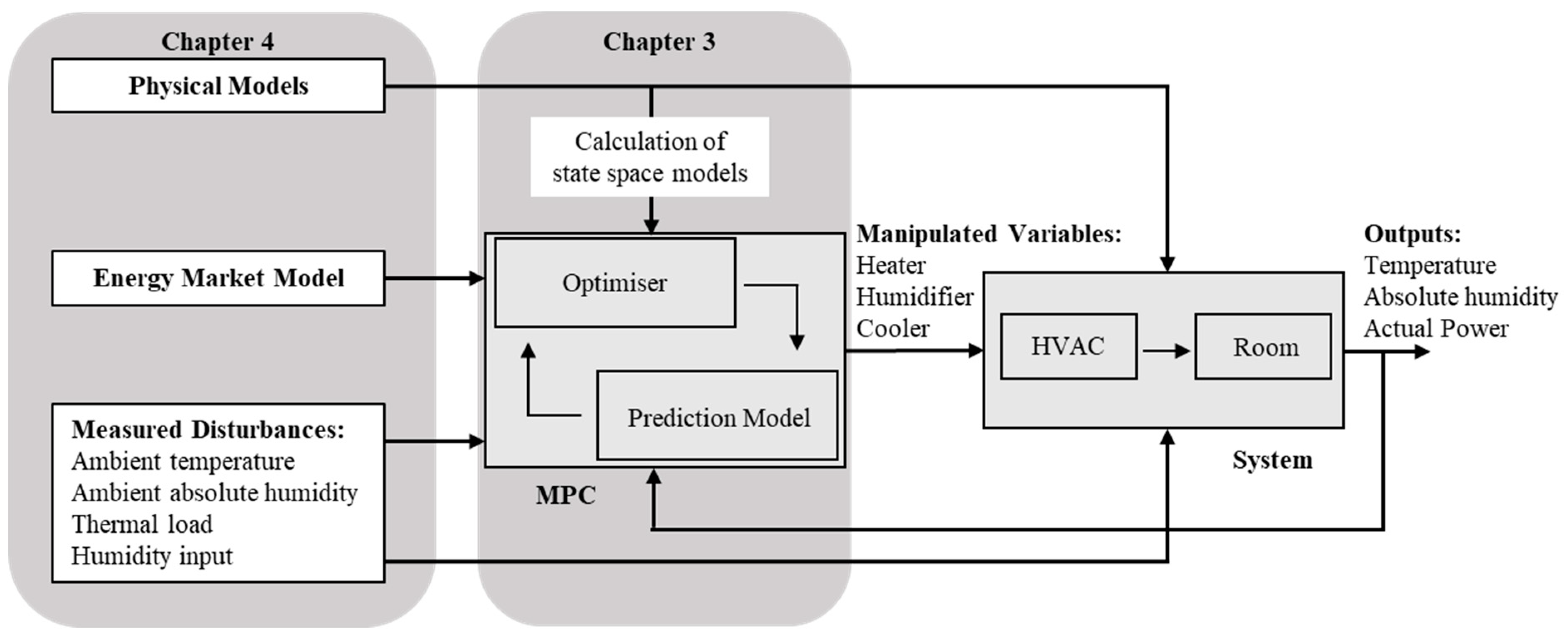
The system to be controlled consists of physical models of a building and an HVAC system, which are described in detail in Section 4. From these physical models, linear, time-discrete state space models are derived, which function as prediction models as part of the MPC, as shown in Figure 1. Using the optimisation algorithm, optimised control signals adapted to the boundary conditions are transmitted to the system to be controlled. The MPC directly controls the heating and cooling coil as well as the humidifier with control signals (manipulated variables). The control signals are limited between 0 and 1. The fans are not controlled via MPC and are operated with a constant volumetric flow of 2000 m3/h. The condition of the supply air is composed of fresh air conditions and the respective conditioning of the climate functions controlled via the control variables. The temperature and humidity of the indoor air are calculated from the proportion of indoor air, supply air, and outdoor temperature. The theoretical basis and configurations of the MPC are described in more detail in Section 3.
A schematic overview of the structure and the functionality of the MPC is given in Figure 1.
Air cooling in the model is realised with one of two processes: Either a dehumidification process (condensate formation) or dry cooling (without condensate formation) is applied. This behaviour cannot be represented in one linear system since a latent phase transition occurs after reaching the saturation temperature. Consequently, for both cases, a multiple model predictive controller with two different prediction models is used in the following. If condensate formation occurs, the prediction model A is switched over to the prediction model B. The two prediction models are based on a multiple model predictive controller. The two prediction models are generated around different operating points (with and without condensation) by linearizing the whole model. Due to the thermal inertia of the system, a time step of 900 s is applied.
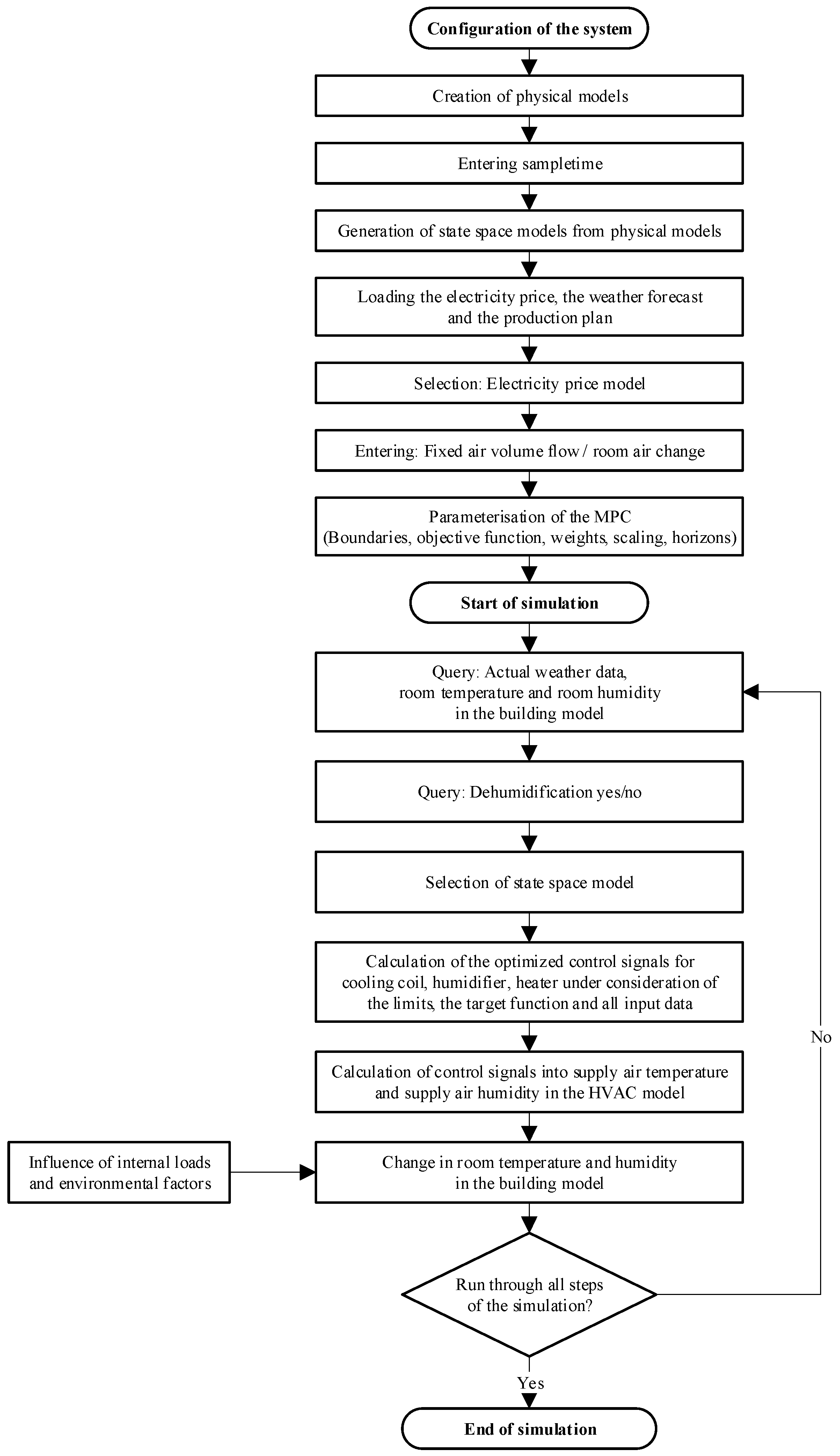
The following flowchart (Figure 2) provides a graphical overview of the procedure for creating, parameterizing, and the functioning of the MPC.
3.1. Time Discrete State Space Model
The developed MPC uses time-discrete LTI systems instead of time-continuous systems. Hence, the equation of state does not describe the derivative (t) of the states, but the states of discrete, future sampling times, x(k+1). The matrices AD (state matrix) and BD (input matrix) of the time-discrete state space representation result from the general solution of the temporal course of the state variable x from time t0.
Accordingly, the matrices AD and BD are formed at the sampling times T. The sampling time is the duration of a time step in the discrete system. The matrices C (output matrix) and D (feedthrough matrix) remain unchanged in comparison to the time continuous system [27,28]:
The time-discrete representation used is as follows:
3.2. Optimisation Problem and Solution Methods
The core of the developed MPC is an optimisation algorithm for calculating the optimal control variable sequence :
The deviations of the actual values from the target values of the controlled system are minimised over the prediction horizon, taking restrictions into account. The objective function ) consists of four parts:
Output Reference Tracking:
Manipulated Variable Tracking:
Manipulated Variable Move Suppression:
Constraint Violation:
The output variables can be described with the internal prediction model, the current states and inputs . From this, it follows that the objective function ) depends only on the decision variable [23].
In each step of a sequence , an approximate quadratic subproblem is formed from the first and second derivatives of the objective function at point .
By defining weights and scales, the aggressiveness of the control signals can be adjusted by defining the suppression of changes.
The described objective function is minimised by the method of sequential quadratic programming (SQP), which is an extension of quadratic programming (QP) and one of the most effective methods for solving nonlinear and nonlinear-restricted optimisation problems [29].
3.3. Multiple Model Predictive Control
In order to keep the deviations between a linear model for control and the real system small over a larger working range, there is the possibility of multiple model predictive control (MMPC). With the MMPC, several controllers with different internal models and parameters are combined in a block and selected via an additional input (“switch”). Depending on the environmental and operating conditions, the most suitable time-discrete state space model can be selected to calculate the optimum control variable sequence for the system.
3.4. Economic Model Predictive Control
The aim of the economic, model-predictive regulation is to minimise monetary costs. The objective function is formulated in such a way that the current and predicted electricity price multiplied by the current and predicted output over the prediction horizon, p, is minimised. The suppression of changes in the control variables, , and the minimisation of restriction violations, , remain the same in comparison to set point compliance or energy optimisation.
The room temperature and absolute humidity of the room air are kept above restrictions in the comfort field.
4. Model Description
In this section, the analysed system based on a real confectionery manufacturer and the models used to calculate flexibility and savings potentials are described. The system consists of a packaging hall for chocolate bars, which are cooled by a novel, local air-conditioning system introduced by Heidrich et al. [15] and a connected air-conditioning system for providing conditioned air to the rest of the hall within the limits of the comfort field for workers.
Without local air-conditioning of the chocolate bars, the entire hall must be air-conditioned to 18 °C and 50% relative humidity in order to avoid deformation of the chocolate, condensation effects on the chocolate bar, and problems with electrostatic charging of the packaging cardboard [17,30,31].
In the hall, there are also packaging machines and medium-heavy working staff emitting heat and water. The number of staff depends on the shift (production in operation, no production, cleaning shift).
In order to be able to model the hall, extensive measurements were carried out and physical models of the hall and the technical building equipment were created in MATLAB/SIMLUNK. The most important parameters for modelling the system can be found in Table 1.
The models used for the room, the air conditioning system and the boundary parameters (internal loads, electricity prices, weather) are described below.
4.1. Physical Building Model
The physical room model used is based on a building model from the open source CARNOT toolbox (Conventional and Renewable Energy Systems Optimisation Toolbox) [33].
The thermal heat-up and cooling behaviour is calculated by integrating the heat flow balance divided by the thermal storage capacity of the building mass over time.
The change of the absolute air humidity is calculated analogously to the thermal behaviour.
4.2. Physical Air Conditioning System Model
The HVAC system consists of an electric pre- and post-heater, a cooling register, which is supplied with cold water by a compression chiller, an electrically operated steam humidifier, and a supply and exhaust fan and is operated with 100% fresh air.
The HVAC simulation model is based on the physical laws of the Mollier diagram [34]. Furthermore, characteristic curves of the manufacturer are used for modelling the cooling supply (compression chiller with flow temperature of −1 °C) and steam humidification (3 bar of saturated steam).
4.3. Boundary Parameters—Internal Load
The internal thermal and water loads necessary for an optimised, model-predictive control of an air conditioning system are determined by real active power measurements of the machines in the hall, calculations for the heat of illumination according to VDI 2078 [34], humidity and heat emission of the persons in the hall according to VDI 2078, and the influence of the local air conditioning by transfer of laboratory results.
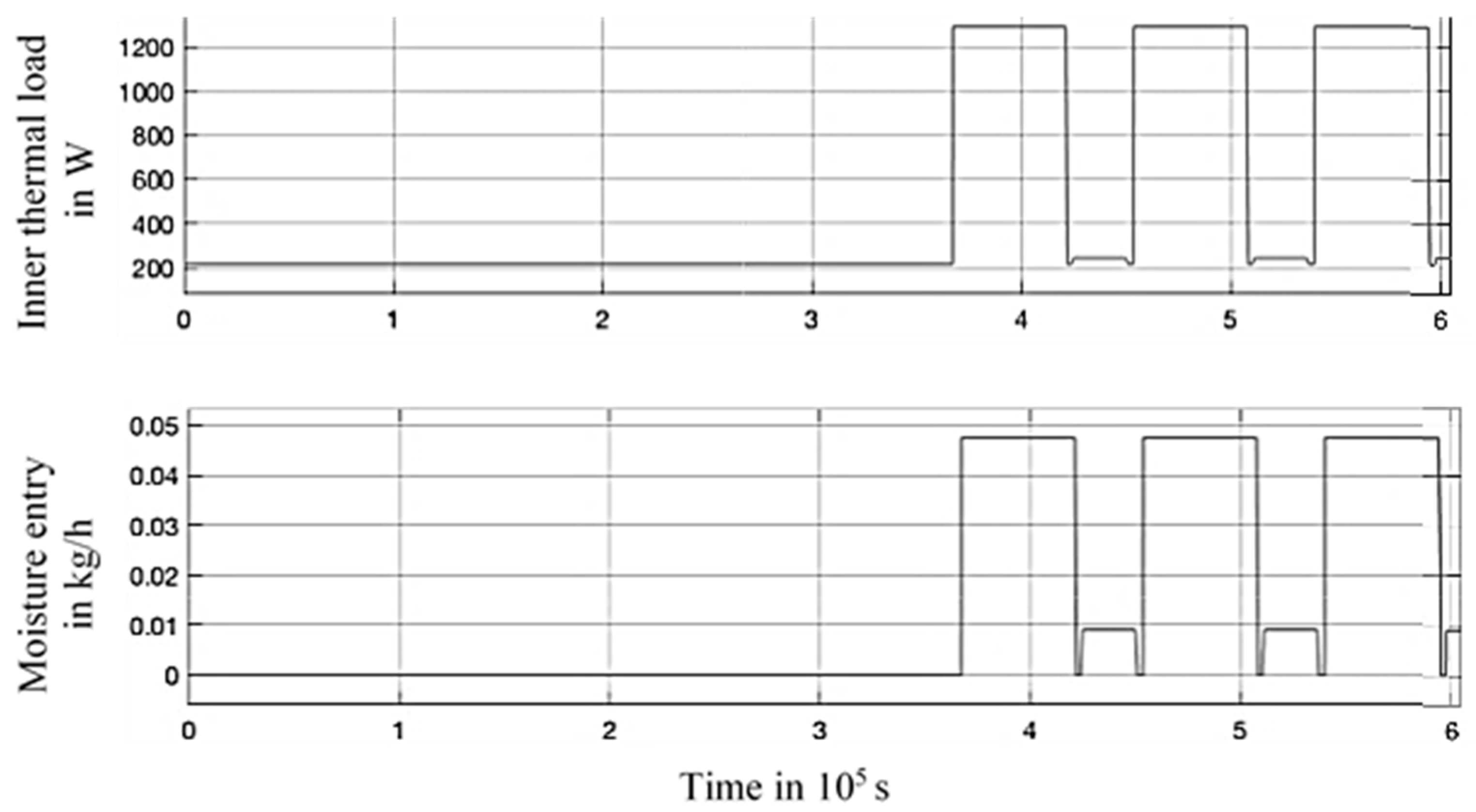
The following figure (Figure 3) shows the temporal course of the determined, smoothed, internal loads as a function of time depending on the production plan. The maximum is reached during running production (three days per week). When production is switched off there is only a low thermal load due to the standby operation of the switch cabinets and machines. During the cleaning shift after every production shift, the room lighting is switched on and a few employees, hard at work, are in the hall.
4.4. Boundary Parameters—Weather Data
The weather data used for simulation and prediction consist of historical hourly values for air temperature and absolute humidity of the surroundings. These are test reference year data of a central German city (i.e., Kassel) in the observation period 1988–2007. Averaged weather data sets are understood as test reference years, which represent a typical weather course of one year. Real forecast values are indispensable for a later, real application operation and can be considered by the developed control. However, historical weather data sets are used to determine savings and flexibility potentials, as these cover a long period of time and reflect the expected value without annual deviations.
4.5. Boundary Parameters—Electricity Price Data
Two electricity price scenarios are defined for the analysis of an economic, model predictive control–a constant and a flexible model:
- In the status quo scenario, a standard, constant total electricity price (13.18 ct/kWh) for industrial customers in Germany is chosen.
- In contrast to that, the second scenario reflects a possible future electricity price model of a dynamized renewable energy levy (EEG levy) and electricity procurement via the day-ahead exchange market in Germany. The current static EEG levy due in Germany, which is levied to promote renewable energies in Germany, is replaced by a dynamic EEG levy, which is calculated using the day-ahead exchange electricity price multiplied by a certain factor.Flexible EEG levy = Day-head electricty price · multipier
This multiplier must be successively recalculated and determined for the differential cost compensation for Germany. For the following simulations, a factor of 1.9 has been defined. Furthermore, limits of the flexible EEG allocation upwards and downwards are foreseen. The upper limit of the dynamic EEG levy consists of twice the German, static EEG levy, the lower limit is 0, and negative electricity prices are no longer possible according to this model [35,36].
In addition to the electricity price, incidental electricity costs are considered in all analysed scenarios corresponding to the average costs of 4.28 ct/kWh for German industrial customers with an annual consumption of 160 to 20,000 MWh [37].
The exchange electricity price generally has two maximums and two minimums per day. Since the loads are to be shifted from a high tariff to a tariff as low as possible, a prediction of at least 12 h is necessary. Regarding a time step of 900 s and a prediction horizon of 12 h, this results in 48 prediction steps. To reduce calculation efforts the control horizon is set to 20 steps, i.e., 5 h.
Comparable to the weather forecast, a real electricity price forecast is also indispensable for real operation. The electricity price forecast is included in the developed MPC approach by downloading real electricity prices from EEX for the next day (day-ahead electricity prices) and script-based further processing. However, as already described in the section on weather forecasting, historical electricity price time series over longer periods are better suited for calculating flexibility and savings calculations.
4.6. MPC Constraints
The constraints used to create the MPC do not vary in all considered scenarios. The constraints include the permissible temperature and humidity limits in the room as well as the control variable limitation. Both the temperature, as well as the air humidity, depend on the limits of an average comfort field. The control variable limitations resulting from the air conditioning system control are as follows:
16 °C ≤ room temperature ≤ 24 °C
0.005 kg/kg ≤ absolute humidity of the room ≤ 0.009 kg/kg
0 ≤ control variable heating/moisture/cooling ≤ 1
4.7. MPC Weights
The different weights of the sub-target functions that are required to create the MPC are described below. In all scenarios, the control variables should not adhere to a value and, therefore, have a weight of 0. The weight of the change suppression of the control variables is set to 0.1. This reduces the too fast upswing and downswing of the control values.
The weightings of the control variables vary depending on the scenarios, which are described in Section 5. A distinction is made between two cases:
- The energy-optimal control keeps the indoor temperature and humidity inside limits in the comfort field. The weights of the first two model outputs (indoor temperature and absolute humidity) are 0. The third output (i.e., power) is to be minimised; hence, it receives a weight of 1.
- The regulation with economic objective function receives the current electricity price as weight for the achievement. This is multiplied by 10, since this setting has a similar weight as that with the energy-optimal regulation and better results are obtained. The temperature and humidity of the room are no longer included in the target function.
5. Scenario Description and Results
In order to evaluate the flexibility and savings potentials, the previously described control variants of the MPC in different seasons are analysed.
The energy demand and the resulting costs of the status quo are given as a reference. In the status quo, PI cascade controllers are used for constant setpoint input of temperature and humidity; the electricity price remains constant at 13.18 ct/kWh. The power consumption and the resulting costs of the status quo are indicated as a reference.
First, three days in January are graphically examined in order to illustrate a possible load shift (scenario I–III). Subsequently, electricity consumption and costs incurred by the three different operating variants are compared over 20 days in January. Since the weather influences change strongly in the summer, the load management potential is finally illustrated by a flexible electricity price and EMMPC for 10 days in July.
The energy-optimal scenario I serves as a comparison for the scenarios in which load management is carried out. Scenarios II and III use the economic objective function in which the current system output multiplied by the current electricity price over the prediction horizon is minimized. In the second scenario, a constant electricity price is assumed, in the third scenario, a flexible electricity price as described above is used. Table 2 shows an overview of the simulated scenarios.
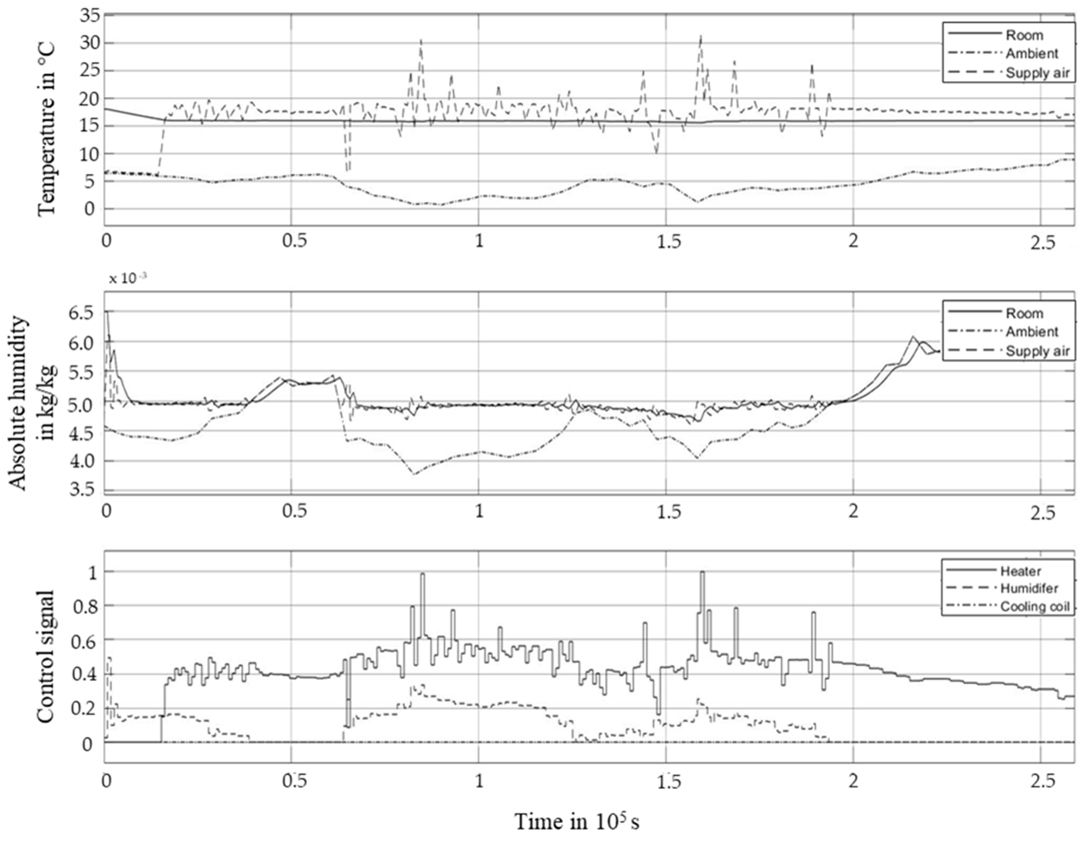
5.1. Scenario I: Energy-Optimised MMPC—3 Days in January
In this scenario, the energy consumption of the air conditioning system is minimized. The weights for temperature and absolute humidity are 0. The comfort field is maintained by the restrictions. The weight for the performance of the system components is 1. The weight for the output of the system components is 1. The target value for the output is 0. Thus, the summed quadratic deviation of the power from 0 over the prediction horizon is minimised.
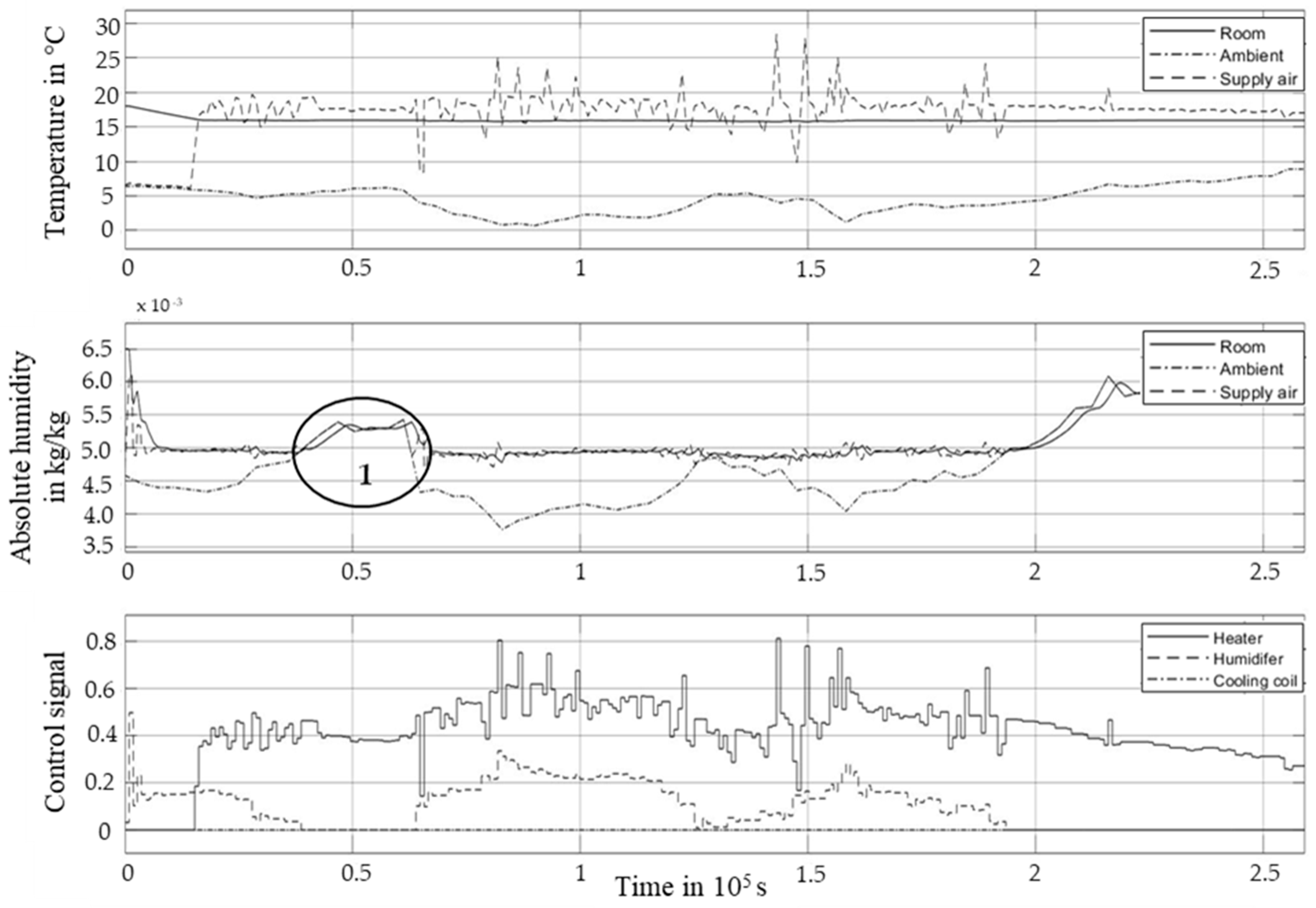
As shown in Figure 4, the room temperature is kept at the lowest limit (16 °C), as this is the least amount of energy required for supply air conditioning. The absolute humidity of the outside air is not raised by the humidifier if it is above the lower limit of 5 g/kg. Since the HVAC system is operated with 100% fresh air from the outside, the absolute humidity of the room, provided that it remains within the specified limits, depends on the conditions of the fresh air, as can be seen in area 1 of Figure 4.
5.2. Scenario II: Cost-Optimised EMMPC with Constant Electricity Price—3 Days in January
In this scenario, the economic objective function is used to minimize costs. The output is multiplied by the current costs in each time step and minimized by adding up the prediction horizon. The electricity price in this scenario is constant at 13.18 ct/kWh. Therefore, this is a simultaneous energetic and economic optimisation. The difference between this regulation and the regulation in scenario I is that the current power consumption of the air conditioning system is no longer included in the target function as a square but linear value. As a result, energy cost peaks are no longer minimized, as they no longer flow disproportionately into the target function.
The behaviour is very similar to the previous scenario I, with slightly changed current reference peaks during operation of the heater, as it is shown in Figure 5.
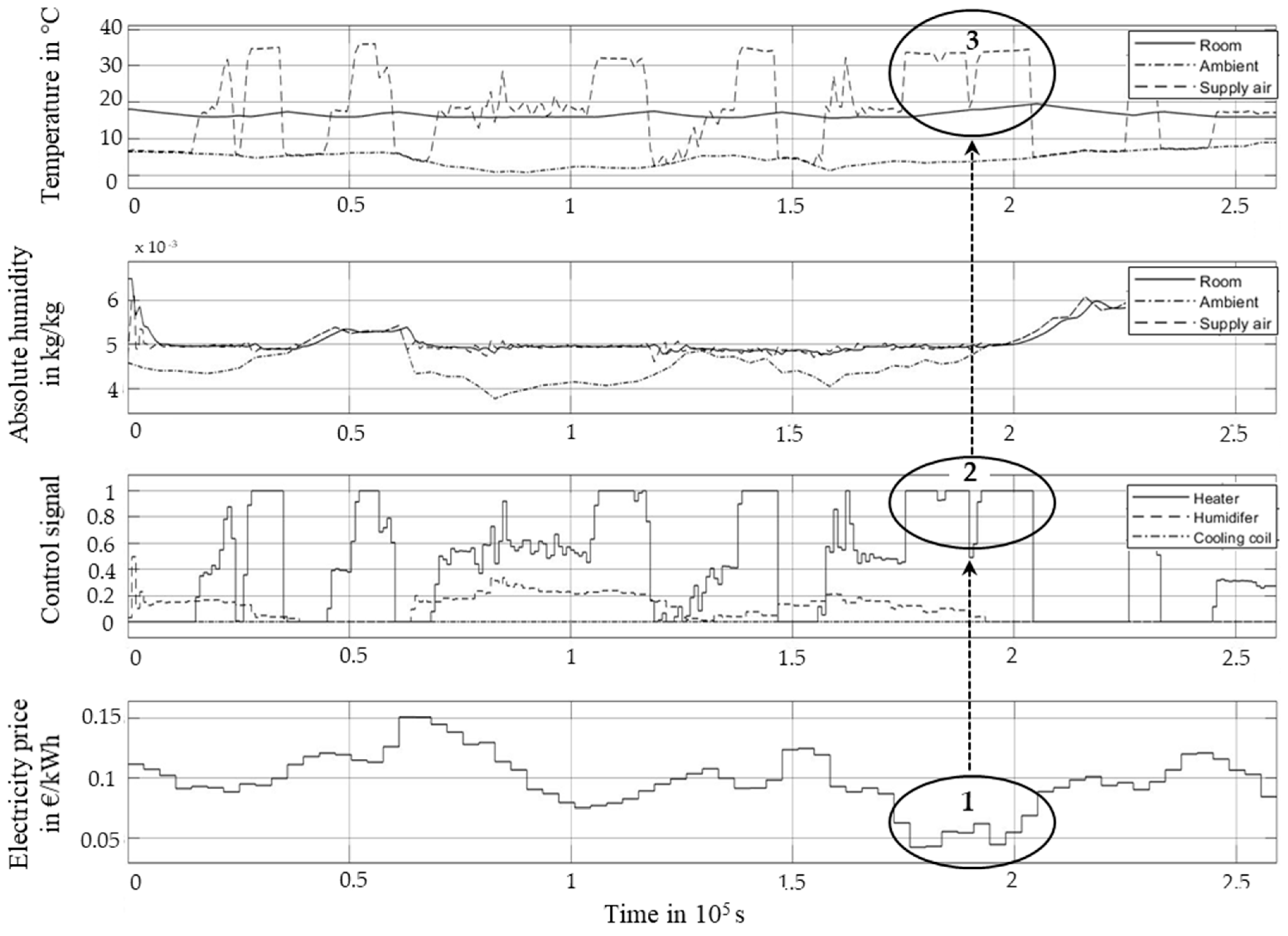
5.3. Scenario III: Cost-Optimised EMMPC with Flexible Electricity Price—3 Days in January
In this scenario, a flexible electricity price is used, as described in Section 4.5. This results in electricity price changes of up to 10 cents, see Figure 6. The indoor temperature varies between 16 and 21 °C. The control variables of the heating coil vary between 0 and 1. Especially in low-price phases, see area 1, Figure 6, and before a sudden price increase, the heating register, see area 2, Figure 6, prematurely heats up the room, see area 3, Figure 6. The humidifier is only activated when the absolute humidity falls below 5 g/kg. Load shifts are possible, as shown in Figure 6.
5.4. Winter Case—Comparison of Control Variants over 20 Days in January
Three scenarios—besides the status quo—were simulated over the first 20 days in January of the reference year. The energy consumption and the energy costs incurred by the air conditioning system are shown in Table 3. The relevant changes are also shown.
In comparison to the status quo, energy savings of around 35% are achieved in the winter case by extending the temperature and humidity limits and using a model-predictive controller. The results of the simulation with dynamic EEG allocation show a reduction in costs of 3.7% compared to the energy-optimal scenario with changed target function and constant electricity price. Compared to scenario II (EMPC with constant electricity price), energy consumption increases slightly using a flexible electricity price model. This higher energy consumption is due to the fact that the room temperature for storing the shifted energy is raised, resulting in higher heat losses which in turn also depend on the insulation of the building.
However, by varying the building weight between 90 and 120 [32], the cost savings increase from 40% to almost 43% compared to the status quo by the use of the EMMPC and a flexible EEG levy in 20 days of January.
5.5. Summer Case—EMMPC with Flexible Electricity Price over 10 Days in July
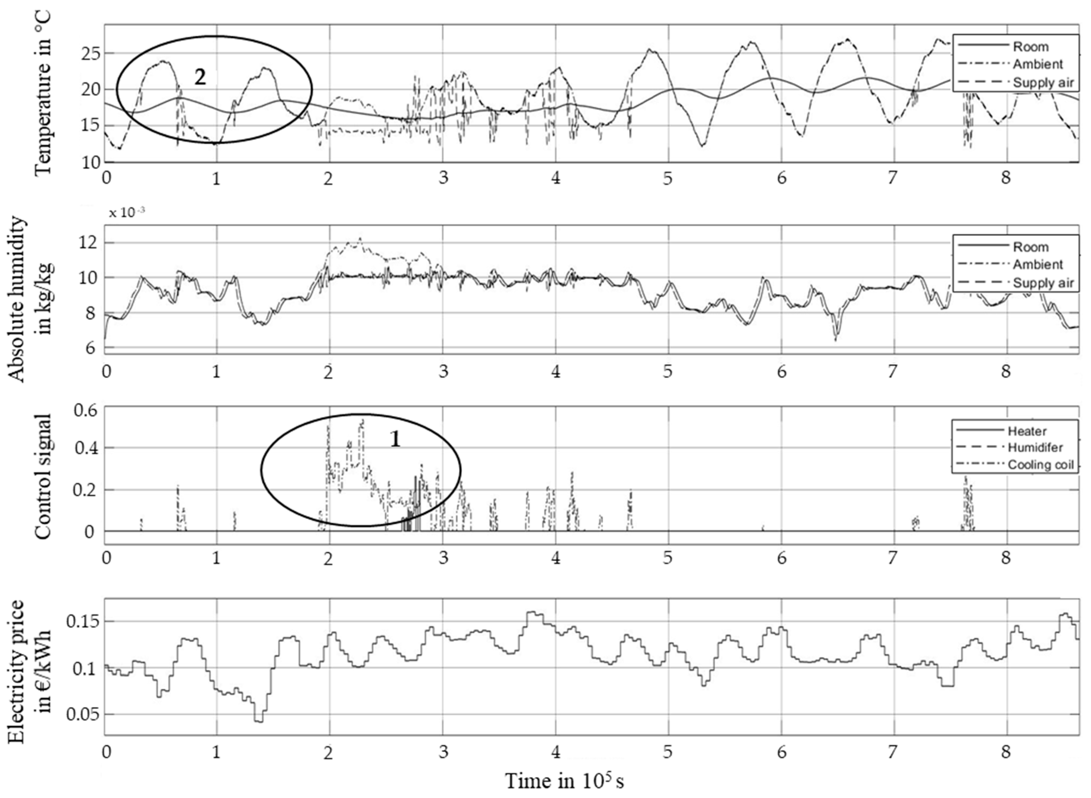
In addition to the winter case, 10 days in summer (days 191–200) are simulated with an electricity price including dynamic EEG allocation (see scenario III). The extent to which the cooling register can contribute to load management is investigated. The results are shown in Figure 7.
In summer, most of the energy is needed to dehumidify the supply air, see area 1, Figure 7. Since the room air is exchanged relatively fast, it is not possible to store energy by shifting the dehumidification output. There is no correlation between the electricity price and the control signal of the cooling register. The outside air is cooled by dehumidification. Therefore, despite high outside temperatures, low inside temperatures must be noted, see area 2, Figure 7. A shift before cooling loads is also not possible, and load management cannot be carried out under such weather conditions.
6. Conclusions and Outlook
The paper illustrates an economic multiple model predictive control of an HVAC that can either meet room temperature and humidity fixed set points targets, minimise energy consumption, or alternatively, minimise economic costs through a flexible electricity pricing model.
The future electricity market model has a significant impact on the results of any flexible energy demand due to the economic incentives. In principle, several different market designs are possible while the presented EMMPC controller focuses on price-based models [13,14]. Doing this, the EMMPC controller acts as a smart responder regarding the economic signal, allowing HVAC systems to participate in the energy market. For the case study, located in Germany, the future flexible electricity pricing model discussed in [35,36] is applied. The approach is transferable to further price-based or to most incentive-based models.
As a case study, a production hall for the packaging of chocolate bars is used, which are locally air-conditioned by a cross-flowing displacement ventilation for conveyor belts, so that the room air condition can be kept within the comfort field with the help of restrictions and does not have to depend on the product requirements of the chocolate (18 °C, 50% relative humidity). Accordingly, the physically possible savings described by Heidrich et al. (2018) [15] can be achieved efficiently and flexibly with the EMMPC controller. The internal loads of the production hall, as well as weather data, influence the system as disturbance variables and are taken into account by the EMMPC controller. To evaluate the EMMPC controller, various scenarios are evaluated considering seasonal influences.
Electricity costs in winter are reduced by around 40% and the energy savings are around 35% compared to the status quo. In comparison to a constant electricity price in the winter case (20 days), the energy consumption in the flexible EEG levy scenario increases slightly due to higher heat losses when the room temperature is temporarily raised. Nevertheless, there are slight cost savings due to the exploitation of low-price phases. It is also shown that a larger thermal storage capacity of the building increases the potential for load shifting.
To sum up, flexible electricity prices with even larger spreads provide correspondingly larger economic incentives for flexible air conditioning in buildings or flexible cooling systems, as is described by Peesel et al. (2018) [38]. Since air-conditioning is used in low-price phases (although this is not always sensible from an energy point of view, e.g., due to the higher transmission heat losses), a conflict of objectives arises between energy savings and economic savings. The use of an energy-optimal control system saves both energy and costs. However, the flexibility to, for example, relieve electricity grids through flexible electricity prices is eliminated.
To control even more complex air conditioning systems in the future, e.g., containing mixed air chambers, which causes even stronger non-linearities in the system behaviour, the extension of the MMPC by further MPC controllers is currently being worked on. In addition, the coupling to a production plan-dependent activation time optimisation adapted to the hall and outdoor air conditions, which determines an optimal start time for the air-conditioning of the hall, is in progress. In this way, energy consumption can be further reduced [16].
In order to demonstrate the functionality in real-life operation also, the coupling with a full HVAC system with a climate chamber, in which internal loads can also be simulated, is under construction. A further starting point is the creation of adaptive, self-learning state space models, which are generated on the basis of real measurement data in order to further improve the prognostic capability and thus the accuracy of the optimal control variables.
The publication shows that the use of an economic model predictive control is suitable for the efficient and economic prognostic guided control of HVAC plants, which participate actively in load management. The approach of a multiple model predictive control can particularly control the non-linear behaviour of typical HVAC processes like dry and wet cooling. Thus, EMMPC is a promising approach to optimise the flexible operation of complex HVAC systems. However, even more in-depth development work is required to map more complex systems on the one hand and to be able to control real systems in real time on the other hand.
Author Contributions
Conceptualization: T.H.; Investigation: J.G. and T.H., Methodology: T.H.; Writing: T.H., J.G. and H.M. Project administration: J.H. Review & editing: T.H. and H.M.
Funding
This research was funded by the German Federal Ministry for Economic Affairs and Energy (FKZ: 03ET1180).
Acknowledgments
The contents of this paper have been acquired within the cooperation project “Smart Consumer—Energy efficiency through systemic coupling of energy flows by means of intelligent measurement and control technology”.
Conflicts of Interest
The authors declare no conflict of interest.
Nomenclature
| : State vector |
| : System input vector |
| : System output vector |
| : State matrix |
| : Input matrix |
| : Output matrix |
| : Feedthrough matrix |
| : Plant output |
| : Manipulated variable |
| J(): Objective function |
| : Number of plant output variables or manipulated variables |
| : Prediction horizon (number of intervals) |
| : Tuning weight |
| : Scale factor |
| : Reference |
| : Current control interval |
| : Constraint violation penalty weight |
| : Slack variable at control interval |
| : Heat flow balance in W |
| : Building mass in kg |
| : Specific heat capacity at constant pressure |
| : Temperature at time t |
| t: Time in s |
| : Total power consumption of the HVAC system (without fan power consumption) in kW |
| : Electricity price in |
References
- United Nations. Climate Change. Available online: http://www.un.org/en/sections/issues-depth/climate-change (accessed on 3 October 2018).
- NASA. Global Climate Change—Vital Signs of the Planet. Available online: https://climate.nasa.gov/ (accessed on 3 October 2018).
- Pachauri, R.K.; Mayer, L. (Eds.) Climate Change 2014. Synthesis Report; Intergovernmental Panel on Climate Change: Geneva, Switzerland, 2015; ISBN 978-92-9169-143-2. [Google Scholar]
- Patwardhan, A.P.; Gomez-Echeverri, L.; Nakićenović, N.; Johansson, T.B. (Eds.) Global Energy Assessment (GEA); Cambridge University Press: Cambridge, UK, 2012; ISBN 9780521182935. [Google Scholar]
- D&R International Ltd. 2011 Buildings Energy Data Book; Pacific Northwest National Laboratory: Richland, WA, USA, 2012. [Google Scholar]
- Pérez-Lombard, L.; Ortiz, J.; Pout, C. A review on buildings energy consumption information. Energy Build. 2008, 40, 394–398. [Google Scholar] [CrossRef]
- Hitchin, R.; Pout, C.; Butler, D. Realisable 10-year reductions in European energy consumption for air conditioning. Energy Build. 2015, 86, 478–491. [Google Scholar] [CrossRef]
- Zhang, K.; Zhang, X.; Li, S.; Jin, X. Review of underfloor air distribution technology. Energy Build. 2014, 85, 180–186. [Google Scholar] [CrossRef]
- Guyot, G.; Sherman, M.H.; Walker, I.S. Smart ventilation energy and indoor air quality performance in residential buildings: A review. Energy Build. 2018, 165, 416–430. [Google Scholar] [CrossRef]
- Nardi, I.; Lucchi, E.; Rubeis, T.; de Ambrosini, D. Quantification of heat energy losses through the building envelope: A state-of-the-art analysis with critical and comprehensive review on infrared thermography. Build. Environ. 2018, 146, 190–205. [Google Scholar] [CrossRef]
- Meschede, H. Increased Utilisation of Renewable Energies through Demand Response in the Water Supply Sector; case study: Rio de Janeiro, Brazil, 2018. [Google Scholar]
- Khripko, D.; Morioka, S.N.; Evans, S.; Hesselbach, J.; de Carvalho, M.M. Demand Side Management within Industry: A Case Study for Sustainable Business Models. Procedia Manuf. 2017, 8, 270–277. [Google Scholar] [CrossRef]
- Palensky, P.; Dietrich, D. Demand Side Management: Demand Response, Intelligent Energy Systems, and Smart Loads. IEEE Trans. Ind. Inf. 2011, 7, 381–388. [Google Scholar] [CrossRef] [Green Version]
- Sharifi, R.; Fathi, S.H.; Vahidinasab, V. A review on Demand-side tools in electricity market. Renew. Sustain. Energy Rev. 2017, 72, 565–572. [Google Scholar] [CrossRef]
- Heidrich, T.; Alimi, A.; Grothues, L.; Hesselbach, J.; Wünsch, O. Cross-flowing displacement ventilation system for conveyor belts in the food industry. Energy Build. 2018, 213–222. [Google Scholar] [CrossRef]
- Heidrich, T.; Dunkelberg, H.; Weiß, T.; Hesselbach, J. (Eds.) Flexibilization of Energy Supply Using the Example of Industrial Hall Climatization and Cold Production; Simulation in Production and Logistic; Kassel University Press GmbH: Kassel, Germany, 2017. [Google Scholar]
- Wagner, J. Lokale Klimatisierung Temperatursensibler Produkte; Dissertation; Kassel University Press: Kassel, Germany, 2016; ISBN 9783737650052. [Google Scholar]
- Heidrich, T. Energieeffizienzsteigerung in der Süßwarenindustrie durch lokale Klimatisierung und systemische Kopplung von Energieströmen. Innov. Energy Technol. Food Ind. 2016. [Google Scholar] [CrossRef]
- Afram, A.; Janabi-Sharifi, F. Theory and applications of HVAC control systems—A review of model predictive control (MPC). Build. Environ. 2014, 72, 343–355. [Google Scholar] [CrossRef]
- Naidu, D.S.; Rieger, C.G. Advanced control strategies for HVAC&R systems—An overview: Part II: Soft and fusion control. HVAC&R Res. 2011, 17, 144–158. [Google Scholar] [CrossRef]
- Ruano, A.E.; Pesteh, S.; Silva, S.; Duarte, H.; Mestre, G.; Ferreira, P.M.; Khosravani, H.R.; Horta, R. The IMBPC HVAC system: A complete MBPC solution for existing HVAC systems. Energy Build. 2016, 120, 145–158. [Google Scholar] [CrossRef]
- Früh, K.F.; Schaudel, D.; Maier, U.; Bleich, R. Handbuch der Prozessautomatisierung. Prozessleittechnik für verfahrenstechnische Anlagen; DIV Dt. Industrieverl.: München, Germany, 2015; ISBN 978-3-8356-3372-8. [Google Scholar]
- Ma, Y.; Kelman, A.; Daly, A.; Borrelli, F. Predictive Control for Energy Efficient Buildings with Thermal Storage: Modeling, Stimulation, and Experiments. IEEE Control Syst. 2012, 32, 44–64. [Google Scholar] [CrossRef]
- Belic, F.; Hocenski, Z.; Sliskovic, D. HVAC Control Methods—A review. In Proceedings of the 19th International Conference on System Theory, Control and Computing (ICSTCC), Cheile Gradistei, Romania, 14–16 October 2015. [Google Scholar] [CrossRef]
- Bemporad, A.; Morari, M.; Ricker, N.L. Model Predictive Control Toolbox—Getting Started Guide; The MathWorks Inc.: Natick, MA, USA, 2017. [Google Scholar]
- Bemporad, A.; Morari, M.; Ricker, N.L. Model Predictive Control Toolbox—User’s Guide; The MathWorks Inc.: Natick, MA, USA, 2017. [Google Scholar]
- Lunze, J. Regelungstechnik; Springer Vieweg: Berlin, Germany, 2014; ISBN 978-3-642-53943-5. [Google Scholar]
- Lunze, J. Regelungstechnik 1. Systemtheoretische Grundlagen, Analyse und Entwurf einschleifiger Regelungen; Springer: Berlin, Germany, 2007; ISBN 978-3-540-70790-5. [Google Scholar]
- Nocedal, J.; Wright, S.J. Numerical Optimization; Springer Science+Business Media LLC: New York, NY, USA, 2006; ISBN 978-0387-30303-1. [Google Scholar]
- Schirmer, S.; Heidrich, T.; Wagner, J.; Hesselbach, J. Steigerung der Energieeffizienz einer klimatisierten Produktionshalle. HLH 2016, 67, 38–40. [Google Scholar]
- Wagner, J.; Schäfer, M.; Schlüter, A.; Harsch, L.; Hesselbach, J.; Rosano, M.; Lin, C.-X. Reducing energy demand in production environment requiring refrigeration—A localized climatization approach. HVAC&R Res. 2014, 20, 628–642. [Google Scholar] [CrossRef]
- German Engineering Standard. DIN V 18599-2: 2011-12-Energy Assessment of Buildings—Calculation of the Useful, Final and Primary Energy Demand for Heating, Cooling, Ventilation, Domestic Hot Water and Lighting—Part 2: Useful Energy Demand for Heating and Cooling of Building Zones. Available online: https://infostore.saiglobal.com/store/Details.aspx/Details.aspx?ProductID=1504363&timerOff=1&refs=1 (accessed on 3 October 2018).
- FH Aachen. CARNOT Toolbox 2018. Available online: https://de.mathworks.com/matlabcentral/fileexchange/68890-carnot-toolbox (accessed on 3 October 2018).
- VDI-Wärmeatlas; Gesellschaft Verfahrenstechnik und Chemieingenieurwesen; Springer Vieweg: Berlin, Germany, 2013; ISBN 9783642199813.
- Frontier Economics. Costs and Benefits of Dynamizing Electricity Price Components as a Means of Making Demand More Flexible; BMWi: Berlin, Germany, 2016. [Google Scholar]
- Clausen, T. Der Spotmarktpreis als Index für eine dynamische EEG—Umlage; AG Flexibility of the BMWi: Berlin, Germany, 2014. [Google Scholar]
- Federal Association of Energy Consumers (BDEW). Composition of electricity prices for industry in Germany in 2016 and 2017. Available online: https://de.statista.com/statistik/daten/studie/168571/umfrage/strompreis-fuer-die-industrie-in-deutschland-seit-1998/ (accessed on 3 October 2018).
- Peesel, R.H.; Schlosser, F.; Schaumburg, C.; Meschede, H.; Dunkelberg, H.; Walmsley, T.G. Redictive Simulation-based Optimisation of Cooling System Including a Sprinkler Tank. Chem. Eng. Trans. 2018, 70, 349–354. [Google Scholar] [CrossRef]
Figure 1.
Schematic structure of the model predictive control system.

Figure 2.
Flow chart—from configuration of the MPC to simulation run.

Figure 3.
Scaled internal loads of the production hall over seven days.

Figure 4.
Energy-optimised MMPC over three days in January.

Figure 5.
Energy-optimised and cost-optimised economic multiple model predictive control (EMMPC) with constant electricity price over three days in January.
Figure 5.
Energy-optimised and cost-optimised economic multiple model predictive control (EMMPC) with constant electricity price over three days in January.

Figure 6.
Cost-optimised EMPC with flexible electricity price over three days in January.

Figure 7.
Cost-optimised EMPC with an electricity price with dynamic EEG allocation over ten days in summer.
Figure 7.
Cost-optimised EMPC with an electricity price with dynamic EEG allocation over ten days in summer.


Table 1.
Important key parameters of the modeled packaging hall.
| Parameter Packaging Hall | Value | Unit |
|---|---|---|
| Room volume | 800 | |
| Supply air volume flow | 2000 | |
| Heat transfer coefficient walls/ceiling | 0.28 | |
| Heat transfer coefficient floor | 1.00 | |
| Ground temperature | 15 | |
| Storage capacity, medium according to DIN V 18599-2 [32] | 90 | |
| Inner thermal load (during production) | 1292 | |
| Humidity entry max. (during production) | 48 |
Table 2.
Overview of the simulated scenarios with optimised HVAC (heating, ventilation, and air conditioning) control.
Table 2.
Overview of the simulated scenarios with optimised HVAC (heating, ventilation, and air conditioning) control.
| Scenario | Objective Function | Weights [temp. humidity power/costs] |
|---|---|---|
| I. Energy-optimised MMPC | energy-optimised | [0 0 1] |
| II. EMMPC with constant electricity price | economic-optimised | [0 0 ] |
| III. EMMPC with flexible electricity price | economic-optimised | [0 0 ] |
Table 3.
Energy consumption and costs over 20 days in January under different scenarios.
| Scenario | 20 Days | ||
|---|---|---|---|
| Consumption in kWh | Costs in € | ||
| Status quo (18 °C, 50% rel.h) | 7677.5 | 1011.89 | |
| I | Energy-optimised MPC | 6586.6 | 868.12 |
| Change: status quo I | −34.70% | −36.63% | |
| II | EMPC with constant electricity price | 6369.4 | 823.82 |
| Change: status quo II | −36.85% | −39.86% | |
| III | Flexible EEG-Levy | 6566.3 | 817.12 |
| Change: status quo III | −34.90% | −40.32% | |
© 2018 by the authors. Licensee MDPI, Basel, Switzerland. This article is an open access article distributed under the terms and conditions of the Creative Commons Attribution (CC BY) license (http://creativecommons.org/licenses/by/4.0/).
Share and Cite
MDPI and ACS Style
Heidrich, T.; Grobe, J.; Meschede, H.; Hesselbach, J. Economic Multiple Model Predictive Control for HVAC Systems—A Case Study for a Food Manufacturer in Germany. Energies 2018, 11, 3461. https://doi.org/10.3390/en11123461
AMA Style
Heidrich T, Grobe J, Meschede H, Hesselbach J. Economic Multiple Model Predictive Control for HVAC Systems—A Case Study for a Food Manufacturer in Germany. Energies. 2018; 11(12):3461. https://doi.org/10.3390/en11123461
Chicago/Turabian StyleHeidrich, Tobias, Jonathan Grobe, Henning Meschede, and Jens Hesselbach. 2018. "Economic Multiple Model Predictive Control for HVAC Systems—A Case Study for a Food Manufacturer in Germany" Energies 11, no. 12: 3461. https://doi.org/10.3390/en11123461
Note that from the first issue of 2016, this journal uses article numbers instead of page numbers. See further details here.