Aggregating Large-Scale Generalized Energy Storages to Participate in the Energy and Regulation Market

Key Laboratory of Control of Power Transmission and Conversion of Ministry of Education, Department of Electrical Engineering, Shanghai Jiao Tong University, Shanghai 200240, China
*
Author to whom correspondence should be addressed.
Energies 2019, 12(6), 1024; https://doi.org/10.3390/en12061024
Submission received: 5 February 2019
/
Revised: 4 March 2019
/
Accepted: 12 March 2019
/
Published: 15 March 2019
(This article belongs to the Collection Smart Grid)
Abstract
:This paper proposes a concept of generalized energy storage (GES) to facilitate the integration of large-scale heterogeneous flexible resources with electric/thermal energy storage capacity, in order to participate in multiple markets. First, a general state variable, referred to as the degree of satisfaction (DoS), is defined, and dynamic models with a unified form are derived for different types of GESs. Then, a real-time market-based coordination framework is proposed to facilitate control, as well as to ensure user privacy and device security. Demand curves of different GESs are then developed, based on DoS, to express their demand urgencies as well as flexibilities. Furthermore, a low-dimensional aggregate dynamic model of a GES cluster is derived, thanks to the DoS-equality control feature provided by the design of the demand curve. Finally, an optimization model for large-scale GESs to participate in both the energy market and regulation market is established, based on the aggregate model. Simulation results demonstrate that the optimization algorithm could effectively reduce the total cost of an aggregator. Additionally, the proposed coordination method has a high tracking accuracy and could well satisfy a diversified power demand.
1. Introduction
The increasing integration of distributed energy resources (DERs) threatens the stability and reliability of power system operation [1]. With the development of smart grid technologies, the control of flexible loads, such as thermostatically controlled loads (TCL), electric vehicles (EV), and electric energy storages (EES), has become a promising research field to address the problem introduced by DERs [2,3]. Due to the great variety, large scale, wide distribution, and small individual capacity of flexible loads, load aggregators (LAs) are required for the dispatch of such loads and provide flexible services to the power grid.
For LAs, at least two major challenges can be identified. One challenge arises from the diversity of flexible resources. Although co-ordination strategies have recently been studied extensively, most approaches can only be applied to a single device class, such as EV [4], fixed-frequency air-conditioners (FFA) [5], and inverter air-conditioners (IVAs) [6]. An LA should provide different interfaces to integrate different types of resources, which makes it difficult for the LA to fully utilize flexibility of the various flexible resources and increases the control cost. Some papers develop unified models for the co-ordination of different types of resources [2,3], which depend on centralized control. Such methods may not be suitable for the coordination of large-scale flexible loads, since LA should collect detailed parameters of all controlled loads and specify the response power of each load, which has a heavy computational burden and communication traffic, and may lead to privacy issues and device security problems. Recently, the concept of a generalized battery or generalized energy storage (GES) has emerged, to provide a battery-like dispatch interface for reduced-order flexible load models. However, most of the generalized battery models still focus on a single device class, such as FFA [5,7,8,9,10,11,12,13,14], IVA [6] and EV [15]. Developing a generalized battery model for multiple device classes is very challenging, due to the heterogeneous parameters and different operating characteristics across the population. There are several works that present generalized battery models for multiple device classes. However, they either do not consider some important load class, such as IVA [2,16,17], or can only be applicable to ON/OFF controlled devices [18].
The objective of LAs is to provide various flexible services to the power grid. The other challenge arises from the different time scales required by different services; for example, 2–6 s for fast regulation services [19] and 1 h for energy optimization services [2,6,20,21,22]. As different aggregate models typically focus on a single time granularity, most existing studies only considered a single market, such as the regulation market [5], or the energy market [4,6]. It is pointed out, in [23], that since different services have different requirements, participating in multiple markets helps to better utilize the control flexibility of resources and obtain more benefits. To stack multiple services, energy storage systems were controlled, in [24], to simultaneously participate in a contingency requirement, voltage management, and frequency regulation. An optimal control method was presented in [21] for energy storages to provide energy arbitrage, balancing service, capacity value, distribution system deferral, and outage mitigation. The literatures [22,25] co-optimized battery storage for energy arbitrage and frequency regulation. However, these papers only considered traditional energy storages. Although the literature [2] considered the co-ordination of various flexible loads to provide multiple grid services, it had to solve some centralized optimization problems, which may lead to a high computational cost.
To address the above challenges, two levels of GESs are modeled in this paper; namely, a micro GES and a macro GES. A micro GES represents a physical resource with a unified dynamic model and control interface, whereas a macro GES is a cyber entity which captures the dynamics of large-scale GESs. The micro GES model is control-oriented, while the macro GES model is optimization-oriented. When combined together, they can be powerful tools for LAs to deal with the diversity of flexible resources and different time scales of different services. For simplicity of presentation, the term GES refers to micro GES hereafter, unless specially stated. The contributions of our work are threefold:
- (1)
- A general state variable, referred to as the degree of satisfaction (DoS), is defined, and dynamic models with a unified form are developed for heterogenous GESs, including both GESs operating at a continuous power and GESs operating at a discrete power with discrete states.
- (2)
- A unified control framework, based on the market equilibrium mechanism, is presented to co-ordinate heterogenous GESs. General demand curves are constructed under the framework to achieve equal DoS across GESs, and meet diversified requirements and privacy concerns.
- (3)
- A low-dimensional aggregate dynamic model for large-scale GESs, which can be regarded as a macro GES, is derived. A scalable optimization model is then presented for an LA to participate in both the energy market and the regulation market.
The rest of this paper is organized as follows. Section 2 introduces the dynamic model of different GESs. In Section 3, the market-based real-time coordination framework is proposed and demand curve construction methods for GESs are presented. Section 4 derives the aggregate dynamic model for a macro GES. In Section 5, the optimization problem that considers both energy and regulation markets is given. Section 6 shows the simulation results which demonstrate the effectiveness of our method. Finally, Section 7 summarizes our contribution and future work.
2. Dynamic Models for Generalized Energy Storages (GESs)
In this section, the unified dynamic model for different GESs is proposed. This paper focuses on four typical types of GESs (EES, EV, IVA, and FFA), as they account for a large share of flexible resources on the demand side. These resources are called GES as they all can store energy (i.e., electric energy or cold/thermal energy) and, thus, their power consumption could be adjusted without affecting the user satisfaction. Meanwhile, they have similar dynamic characteristics, which makes it possible to establish a unified physical model for them.
2.1. Degree of Satisfaction, DoS
Before establishing the dynamic models, a dimensionless state variable, referred to as the DoS, is defined for GESs, with the following purposes:
- (1)
- It could be used to measure the user satisfaction. The range of DoS is set to [,1], and the closer the DoS is to 0, the higher the user satisfaction is.
- (2)
- DoS could reflect a GES’s state of energy: DoS equalling 0 indicates that the stored energy is at the expected level, while DoS close to ±1 means the stored energy is near the allowed range.
- (3)
- Since a GES can deviate from its ideal state (DoS=0) to provide services, the DoS can be used to quantify its current flexility (i.e., a DoS value close to 0 implies a high flexibility reservation).
- (4)
- As DoS is a generalized index, it can be used to establish a unified model for various GESs.
2.2. Derivation of Dynamic Models
2.2.1. Electric Energy Storage (EES)
To facilitate the establishment of a unified dynamic model, the charge/discharge efficiency of EES is ignored. The dynamic model of an EES is given by:
where and denote the electric energy and power of EES i at time k, respectively ( when EES is charging); and is the control cycle.
The variable S is, hereafter, used to denote DoS. The definition of EES DoS is given by:
2.2.2. Electric Vehicle (EV)
The physical model of an EV is:
where and denote the electric energy and power of EV i at time k, respectively; and is the charge efficiency.
According to the current charger technology, we focus on the prevailing EV type, which operates at two discrete states, idle and charging with a fixed rate [26,27]. Let denote the target energy of EV i at user-specified departure time , and denote the energy at the time EV i is connected into power grid . The average power required to charge EV i to can be calculated by:
If EV i charges at , the expected energy profile is:
An EV can provide its flexibility by deviating from . Referring to the hysteretic model in [28], the DoS of EV is defined as:
where denotes the nominal capcity of EV i; and denotes the energy deadband, which limits the error between and the actual energy at within .
2.2.3. Inverter Air-Conditioner (IVA)
Without loss of generality, cooling air-conditioners are studied in this paper. The thermal dynamic process is modelled by a first-order differential equation [5,6] as:
where and denote the indoor air temperature and outdoor temperature at time k, respectively; is the heat rate of IVA i; and the thermal parameter is .
The analytical solution of Equation (9), in recursive form, is:
The electrical model of an IVA adopts the simplified linear model in [6], which is given by:
where denotes the electric power of IVA i; is the operation frequency of the compressor; and , , , and are coefficients.
The DoS of an IVA is defined as:
where denotes the setpoint; and denotes the allowed temperature deviation.
2.2.4. Fixed-Frequency Air-Conditioner (FFA)
The thermal model of an FFA can also be established by Equation (9). Its electrical model is given by:
where is the coefficient of performance. FFA is an ON/OFF controlled load, so its electric power is equal to the nominal power when it is ON and when it is OFF.
2.3. Unified Dynamic Model
The dynamic models of the above GESs can now be represented in a unified form:
where , , and are coefficients of the unified dynamic model.
Mappings between DoS and the original variables of different GESs are summarized in Figure 1. This paper uses a real-time coordination method of GESs, which could make the average DoS of a cluster of GESs approximately equal. In this paper, such a control characteristic is referred to as DoS-equality control, and will be detailed in the next section.
3. Real-Time Coordination Method of Large-Scale GESs
In this section, a market-based real-time control framework to coordinate large-scale GESs is introduced, and the demand curve construction method of different GESs will be detailed.
3.1. DoS-Equality Control Based on Market Equilibrium Mechanism
The coordination method is based on the market equilibrium mechanism. It establishes a virtual market in the aggregator to coordinate large-scale GESs for target tracking [29]. The main stages of the method are:
- (1)
- Bidding: Each GES expresses its urgency and flexibility by constructing a demand curve. The demand curve is denoted by in this paper, which is a non-increasing function.
- (2)
- Aggregating and clearing: LA collects demand curves from all GESs and forms the aggregate demand curve , where N is the number of controlled GESs. Assume the aggregate target power is , then LA can calculate the clearing price by .
- (3)
- Disaggregating: LA broadcasts to all GESs. Each GES responds to locally, according to its demand curve. The response power of GES i can be obtained by .
Following the above steps, the aggregate target power can be allocated among the GESs, thus realizing accurate power tracking. It should be noted that: (1) The target power depends on the application. In this paper, it will be determined by an optimization problem to be discussed in the next section; (2) the clearing price is only a control signal, rather than a price signal. It is dimensionless and its range is set to [,1]. Therefore, it is called the "virtual price" in this paper.
The market-based coordination method highlights the following advantages:
- (1)
- It improves the autonomy of the GES. Each GES can convert its private information (e.g., user preferences, current adjustable range, and security constraints) into a demand curve. Since the demand curves of all GESs have a unified form, it can shield the differences among various GESs and effectively protect user privacy. Besides, the LA does not have permission to directly control the GES, which improves device security.
- (2)
- It simplifies the control of the LA. The LA does not need to specify the type of each GES, and is able to coordinates various GESs through an identical signal (i.e., the virtual price signal ), which significantly reduces control complexity and the requirement of communication bandwidth.
In addition, by appropriately designing the demand curve of different GESs, the DoS-equality control can be realized to obtain the following advantages:
- (1)
- GESs could have the same degree of user satisfaction, regardless of the resource type or capacity, which ensures control fairness. In addition, since the DoS reflects a GES’s state of energy, the DoS-equality control could avoid some GESs going beyond their adjustable range prematurely, thus better utilizing the regulation ability of a GES cluster.
- (2)
- The unique DoS of a GES cluster can be a state variable to derive an aggregate dynamic model, making it possible to treat the whole GES cluster as a virtual storage (i.e., a macro GES), which will be detailed in Section 4.
According to the operation characteristic, the GES can be further classified into two types: GES operating at continuous power (CP-GES) and GES operating at discrete power with discrete states (DP-GES). A CP-GES (e.g., an EES or an IVA) is able to keep its DoS at the desired value by adjusting its operating power, while, for a DP-GES (e.g., an EV, a FFA, or an electric heater), its DoS generally fluctuates within the allowed range. Additionally, the state-switching frequency of a DP-GES should generally be controlled to prolong the device’s lifetime.
The key of the proposed coordination method is the construction of demand curves for different GESs, which will be introduced in the following subsections.
3.2. Demand Curve of a CP-GES
3.2.1. Demand Curve
Let denote the current DoS of GES i. The following construction principle for the demand curve is established in this paper:
where denotes the electric power required to maintain the current over a control cycle.
Remark 1 (DoS-equality control over CP-GESs).
For ease of explanation, the clearing price is assumed to be constant. When , the response power is higher than , leading to the decrease of ; when , is lower than , leading to the increase of ; when , equals , keeping unchanged. Therefore, the values of all GESs following the principle in Equation (17) will approach the control signal .
Based on Equation (17), the demand curve of a CP-GES is constructed, as shown in Figure 2. Note, again, that the price herein is virtual and is limited between and 1. The demand curve consists of five key points. The anchor point A could satisfy the condition in Equation (17). The points B and C are used to keep the DoS within the limits when responding to any clearing price . Thus, and are the minimum and maximum power, respectively, that would not cause the DoS go beyond the limit over a certain period of time (which is set to 5 min in this paper), without considering the operation constraints. The points D and E, which lie on the line AB and the line AC, respectively, are further introduced to guarantee the response power would not exceed the operational constraints. Thus, and are the minimum and maximum power, respectively, that a GES could operate at in a current control cycle.
3.2.2. Characteristic Power
The EES and IVA are typical CP-GESs. They can both adopt the demand curve shown in Figure 2.
An EES’s characteristic power can be calculated by:
where denotes the nominal charging/discharging power; and are charge/discharge efficiency, respectively; and are the minimum and maximum allowed energy, respectively; and is the stored energy at time t.
IVA’s characteristic power can be calculated by:
where and denote the minimum and maximum power, respectively; and the function obtains the electric power that causes the indoor air temperature to change from the current value to the target temperature over a period of time . The derivation of is detailed in Appendix A.
3.3. Demand curve of a DP-GES
3.3.1. Demand Curve
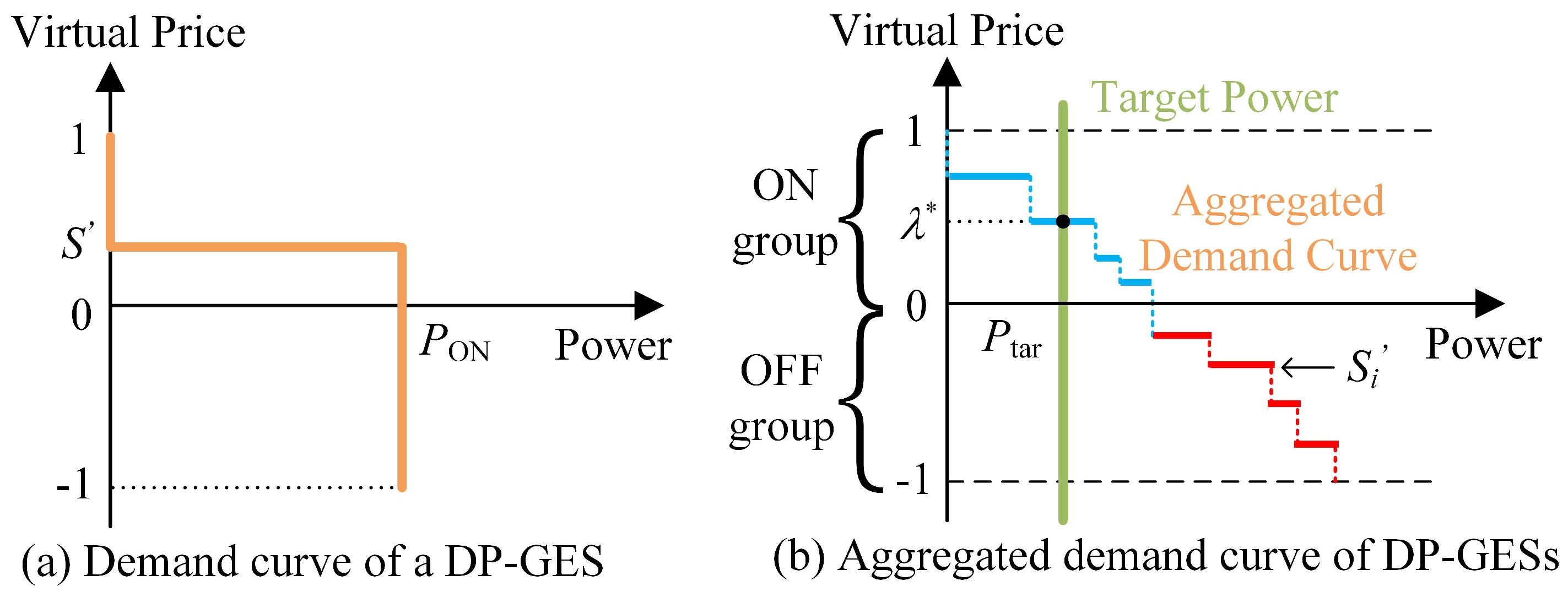
A DP-GES typically has two states; that is, ON and OFF. The proposed demand curve for a DP-GES is illustrated in Figure 3a, where denotes the operating power when the GES is ON, and is transformed from its DoS value by offsetting and then normalizing:
To explain the principle, the aggregate demand curve of a cluster of DP-GESs is shown in Figure 3b, which is obtained by sorting the DP-GESs in descending order of . As can be seen, the proposed bidding strategy can divide the DP-GESs into two groups, according to their operation states (i.e., an ON group in the upper half-plane and an OFF group in the lower half-plane), and achieve the following purposes:
- (1)
- For DP-GESs in the same group, the values of for a given DP-GES reflects its power consumption priority. The higher the value of is, the higher the probability to maintain or switch to the ON state is, and vice versa.
- (2)
- A DP-GES in the ON group always has a higher than that in the OFF group, which gives a high priority for DP-GESs to maintain their current states; thus avoiding frequent switching.
Remark 2 (DoS-equality control over DP-GESs).
For ease of explanation, the trajectory of S and at two different (i.e., and ), are illustrated in Figure 4a,b. Note that the state change of a DP-GES may be triggered either by its value, or by S to ensure comfort. The following laws can be found: When , S ranges in [ + 2,1]; when , S ranges in [,1 + 2], which means that the DoS value fluctuates within a symmetrical range around . Therefore, if the DoS values of the DP-GESs are assumed to be uniformly distributed in such a range, the average DoS of the cluster equals .
3.3.2. Characteristic Power
EV and FFA are typical DP-GESs. They can both adopt the demand curve in Figure 3a.
An EV’s characteristic power is:
where denotes the EV’s nominal charging power.
An FFA’s characteristic power is:
3.4. Locked State
In certain control cycles, a GES may get into the locked state, which means it should maintain its current operating state and power. There are two typical situations: (1) to reduce mechanical wear and protect the device, DP-GESs (such as FFA and EV) should satisfy lockout time constraints before they switch state [30,31]; (2) restricted by the device capability, the response cycle of some GESs may be longer than the real-time control cycle (which is 10 s, in this paper).
The lockout mechanism can be easily realized in this paper, as a GES can simply submit the following demand curve during the lockout time:
which means the response power of GES i maintains its current operating power for any .
4. Aggregate Dynamic Model for Macro GES
One significant advantage of our method is that the aggregate dynamic model of a large-scale GES cluster can be easily derived, thanks to the DoS-equality control feature, as well as the unified dynamic model for different GESs defined in Equation (16).
For CP-GESs, we simply add their dynamic models together:
where represents the set of CP-GESs.
Under the DoS-equality control, the DoSs of all the CP-GESs are approximately equal. Let denote the average DoS of the CP-GES cluster, and denote the aggregate power. The aggregate dynamics of CP-GESs can then be approximated by:
For DP-GESs, to facilitate analysis, we assume the coefficients of their dynamic models to be equal first. Adding their dynamic models together, we obtain:
where represents the set of DP-GESs.
The instantaneous DoS value of each DP-GES is a random variable. Denote the average DoS of DP-GESs as , and denote the aggregate power as . Then, Equation (26) can be written as:
where denotes the number of DP-GESs.
Under the DoS-equality control, of the CP-GESs and of the DP-GESs tend to be equal (i.e., both equal to ) and, thus, can both be denoted by . Therefore, Equations (25) and (27) can be added together:
where denotes the total number of GESs; and is the aggregate power.
Equation (28) forms the dynamics of a macro GES, which can be rewritten, in a compact form, as:
The above derivation is based on the assumption that all DP-GESs have equal model coefficients. For those with different coefficients, we can imagine that DP-GESs are first divided into groups, according to coefficients. Then, aggregation can be carried out in each group by Equation (27) and, finally, the aggregate dynamic model of all of the GESs (including CP-GESs and DP-GESs) is formed by Equation (28).
As described above, an LA can obtain the macro GES model easily by adding teh model coefficients of all GESs with no need to identify GES’s type, thus having a low computational cost. Furthermore, from the control aspect, the low-dimensional aggregate model greatly reduces the complexity of the optimization problem, which will be discussed in the next section.
5. Application
In this paper, the above control methods are applied in the case of multi-market participation. This section will propose an optimization model of multi-market allocation and introduce the overall three-layer control structure.
5.1. Optimal Multi-Market Flexibility Allocation
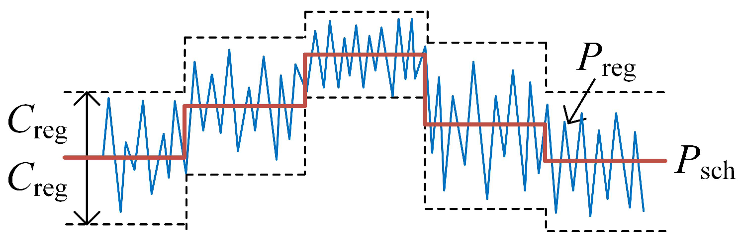
An LA can aggregate the flexibility of large-scale GESs to provide multiple services to a power grid. For example, it can schedule an optimal power consumption profile, according to the electricity price of an energy market [2,6,20], as the profile in Figure 5. LA can provide other ancillary services at the same time to obtain higher benefits [2,20], such as responding to the regulation signal in Figure 5.
The regulation signal can be decomposed into a low frequency part, denoted by regA, and a high frequency part, denoted by regD [32]. The literature [33] analysed the regulation signal of a certain power grid, and found that the high frequency part could account for up to 30%. In this paper, the LA responds to the regD signal, considering the following facts: First, the regD signal has zero-mean over a period of time [32], which could significantly reduce the requirements for the capacity of GESs; second, the extra energy introduced by the regD signal is close to 0, thus having little impact on electricity bills; third, if regulation payments are determined by the performance-based policy used in the Pennsylvania–New Jersey–Maryland (PJM) regulation market [19], the LA could obtain high benefits.
Considering both the energy and regulation markets, the target power of an LA is given by:
where is the hourly scheduled power, which determines the bill paid to the energy market; regD is the regulation signal, normalized to [0,1]; and denotes the contracted regulation capacity.
Let the optimization cycle be 1 hour. Then, the LA solves the following convex optimization problem in the nth cycle to allocate its flexibility to the two markets:
where , , and denote, respectively, the electricity price, regulation capacity price, and regulation mileage price in the kth cycle; denotes the statistical value of the regulation performance score defined by PJM [19], and denotes the statistical value of the regulation mileage [19]; and and are the maximum and minimum power, respectively, of the GES cluster, which are calculated in every optimization cycle as and , where:
Note that EESs are able to discharge and, thus, the LA may sell electricity to power grid at this time. The purchase price and sale price are assumed to be equal in this paper.
The first constraint in Equation (31) is the aggregate dynamic model of the GES cluster; the second constraint ensures the user satisfaction; and the last three constrain the regulation capacity. Thanks to the established aggregate dynamic model, the scale of the GES cluster does not affect the computational complexity of the optimization problem.
To improve user satisfaction, Equation (31) includes a penalty term , which is defined as:
where is a proportionality coefficient, which is assigned as 0.1 here; and is the daily average electricity price.
5.2. Three-Layer Control Structure
To sum up, this paper develops four models; that is, a unified dynamic model and a uniform demand response model for a micro GES, as well as an aggregate dynamic model and an optimization model for an LA to approximate the dynamics of a macro GES and participate in multi-markets. These four models are organized in a three-layer control structure, as illustrated in Figure 6.
(1) Optimization Layer:
At the beginning of the nth optimization cycle, the optimization problem in Equation (31) is solved, and the optimal scheduled power sequence , as well as the regulation capacity sequence , are obtained. The LA implements the first elements of the sequences (i.e., and ) in the current optimization cycle, and repeats the above steps each hour. It is well known that this idea of rolling optimization comes from model predictive control (MPC) [30], which is adopted here to update the aggregate dynamic model iteratively, and to consider constraints in future time slots explicitly.
In each control cycle (10 s in this paper), the LA receives the regulation signal regD from the control center, and then calculates the real-time target power according to Equation (30).
(2) Coordination Layer:
This layer presents a macro GES model to the optimization layer. It aggregates the dynamic models and demand curves of heterogenous GESs, and disaggregates the application-dependent target power by a virtual market, as described in Section 3.1. The clearing price is broadcast to each GES as a coordination signal. The above aggregating and disaggregating methods are application-independent, which implies the flexible resources can provide various (and even stacked) services to the power grid.
(3) Autonomous Device Layer:
In each optimization cycle (1 h), each GES updates its DoS, model coefficients in Equation (16), and power constraints in Equation (32), and then reports this information to the LA. In each control cycle (10 s), each GES reports its flexibility and responds to the clearing price both through the demand curve.
It is worth mentioning that, since the LA interacts with different GESs through a unified set of information—the unified dynamic model, the demand curve, and the virtual price—the method in this paper supports a flexible, tree-like structure. For example, a local concentrator can be deployed in an community to pre-aggregate the information. Therefore, the method has high scalability and is suitable for wide-area coordination of large-scale GESs.
6. Simulation Studies
6.1. Simulation Settings
The simulation cases are based on a residential community system. The simulation lasts for 24 h. The electricity price , regulation capacity price , and mileage price adopt the data in the literatures [6,34], and their profiles are illustrated in Figure 7. The regD signal uses the PJM data on 13 July 2016. According to the statistical analysis on the regD signal in 2016 [35], we set . According to the simulation results based on historical data, we conservatively assign .
Four types of GESs are considered in this paper—EES, EV, FFA and IVA—whose parameters are shown in Table 1; where U(a,b) indicates a uniform distribution between [a,b] and denotes the response cycle of GES. and are the charging and discharging efficiencies, respectively, of EESs in the simulation model. The profile of the outdoor temperature in simulation cases is shown in Figure A1.
To evaluate the control effect, the LA has to estimate the baseline power of the macro GES when all GESs are uncontrolled, which will be denoted by , hereafter. Many papers have studied the estimation method of the baseline load, such as a statistics-based method proposed in [36]. In this paper, since the aggregate model of the macro GES is available to the LA, it can estimate for each hour by solving the following optimization problem:
The solution of Equation (34) is referred to as the baseline case in this paper.
6.2. Case 1: Only Participate in the Energy Market
To evaluate the effectiveness of the aggregate dynamic model and the DoS-equality control, an optimization problem, simplified from Equation (31), which only considers the energy market, is solved:
LA coordinates GESs to cause the aggregate power to track the scheduled power . As illustrated in Figure 8, the proposed method has a high tracking accuracy. In addition, the aggregate power can vary up and down around the baseline power as the electricity price changes, to reduce energy cost. Therefore, the macro GES can be scheduled as virtual energy storage, since it can be charged by making higher than and discharged by making lower than .
Figure 9 demonstrates the performance of the DoS-equality control. As shown in Figure 9a,b, the DoS of all CP-GESs (i.e., IVAs and EESs) can track quite well, as they are able to adjust their power continuously. For DP-GESs (including FFAs and EVs), note again that the average DoS of a cluster, rather than the DoS of an individual, can follow . It can be seen, in Figure 9c, that of the FFAs tracks well. However, for the EVs, slightly fluctuates around . This is because the number of EVs is small, making the statistical characteristics inconspicuous and the distribution of DoS not well-aligned with the analysis in Section 3.3. Therefore, a larger-scale DP-GES cluster yields a better DoS-equality control effect.
Figure 10 shows how well the aggregate dynamic model in Equation (29) fits the cluster with heterogeneous GESs. As can be seen, the values of for all GESs (except EVs) are very close to the aggregate state variable at the end of every optimization cycle. Since the number of EVs is small, especially during 6:00–9:00 and 18:00–20:00 (when some EVs are off-grid), fluctuates around with relatively large errors.
In addition to the small number of DP-GESs, some other factors may also lead to errors in the aggregate dynamic model (e.g., the charge/discharge efficiency is not considered in EES’s dynamic model). In order to prevent the error from being accumulated, this paper adopts the rolling optimization method to mitigate the impacts of these factors continually. As can be observed from Figure 10, when combined with the rolling optimization, the simple aggregate model in Equation (29) could be a useful tool for an LA to capture the aggregate dynamic feature of large-scale GESs, and it enables the LA to treat the GES cluster as a single macro GES in the optimization control.
6.3. Case 2: Participate in Both Energy and Regulation Markets
In Case 2, both the energy and regulation markets are considered. By solving the optimization problem in Equation (31), the scheduled power and regulation capacity can be obtained, as illustrated in Figure 11. For comparison purposes, the scheduled power in Case 1 is also plotted in the figure, which is denoted by . The scheduled power profile in Case 2 has a significant difference from that in Case 1, as the LA allocates the cluster’s flexibility to two markets according to both the electricity price () and regulation price ( and ). As a symmetric regulation signal is used in this paper, can reach its maximum value when . It can be seen that, when is relatively high (e.g., during 14:00–15:00 and 19:00–21:00), the LA tends to maximize to gain higher payments from regulation market.
The target power in this case is calculated by Equation (30), and the tracking performance is shown in Figure 12. The hourly values of and are shown in Figure A2. According to the result, can basically reach 0.95 under the proposed control framework. In comparison, when responding to the regD signal, the value of for a hydroelectric generator can be 0.7∼0.8, while that of an EES can be higher than 0.9 [37]. Therefore, the simulation results demonstrate that the GESs discussed in this paper are very promising alternatives for providing fast and accurate frequency regulation services.
The trajectories of DoS and the clearing price are illustrated in Figure 13. Compared with Figure 10, since the GESs also need to respond to the rapidly changing regD signal, some fluctuations and sudden changes can be observed in , which makes the DoS of GESs unable to exactly follow . However, DoS always tends to approach and, thus, the DoS-equality control is basically realized. In addition, at the end of some optimization cycles (e.g., at 10:00, 16:00, and 24:00), the difference between and is a little larger than that in Figure 10. This is because the regD signal is not exactly zero-mean, which affects the actual energy consumption in each optimization cycle and enlarges the difference.
To analyse the economic benefits of the proposed method, the energy bill, regulation payments, and total cost between the above cases (Cases 1 and 2) and the baseline case are compared. Hourly calculated cost is shown in Figure A3, and Table 2 lists the daily results. As can be observed, Case 1, which only considers the energy market, can significantly reduce the energy bill, when compared with the baseline case. By optimally allocating flexibility in two markets, Case 2 further reduced the total cost, compared to Case 1, even though it received a higher energy bill in the energy market. By providing a fast regulation service, an LA obtained high payments from the regulation market, leading to a significant reduction in the total cost. Therefore, our method could achieve great economic benefits.
6.4. Response Performance of Individual GESs
The proposed control strategy ensures DoS-equality among GESs. For different types of GESs, their response behaviour may be different due to their distinguishing features. To demonstrate this, we pick one GES randomly from each type of GES, and plot their response power in Figure 14.
For CP-GESs, this paper allows different response cycles. For example, an EES adjusts its response power each 10 s ( s), while an IVA adjusts its power every 1 min ( s), considering its response ability; thus, an IVA’s response power is stair-shaped, as shown in Figure 14a.
DP-GESs adjust their response power by regulating the duty cycle. Among them, an EV’s duty cycle at different times is basically similar, as its operation is irrelevant to external conditions and mainly depends on the user’s charging pattern. In contrast, the required power of an FFA varies over time, as it is significantly affected by environmental conditions, such as the outdoor temperature. For example, it can be observed, from Figure 14b, that the duty cycle of an FFA during 13:00–16:00 is higher than that for the rest of the day, as more cooling energy was required during these time slots.
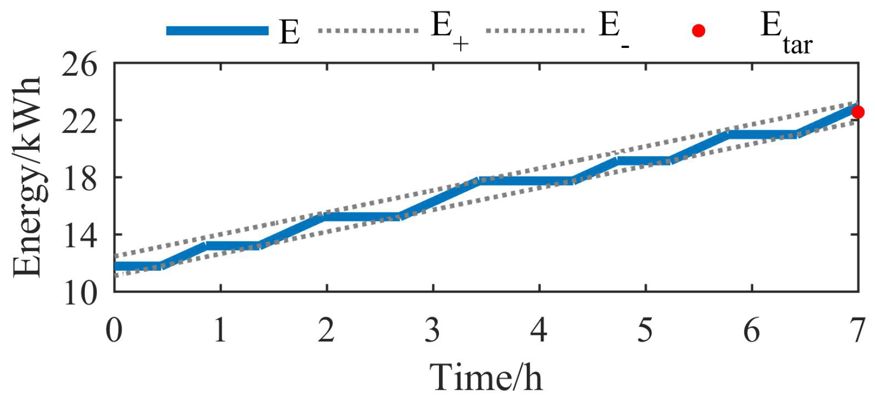
In addition, an EV should ensure that the electric energy reaches its target value at the departure time. The change of electric energy is shown in Figure 15, where and . As we can see, the hysteretic model and control strategy used in this paper can guarantee that the difference between the energy at departure time and the target energy would not exceed .
7. Conclusions
In this paper, a unified coordination method is developed for large-scale heterogeneous GESs, in order to participate in both the energy and regulation markets.
A general state variable, referred to as DoS, is first defined, and dynamic models with a unified form are then developed for different GESs. In real-time control, a market-based coordination framework is adopted, and a DoS-equality control feature is then realized through the construction of demand curves for both CP-GESs and DP-GESs. Based on the unified dynamic models and the DoS-equality control, an aggregate dynamic model for a macro GES is derived. At last, an optimization model, aiming to allocate the flexibility of GESs into both the energy market and the regulation market, is developed, which uses the aggregate model to significantly reduce the mathematical complexity of the optimization problem.
This paper highlights the following advantages: (1) The DoS-equality control feature ensures control fairness amongst different GESs, and better utilizes the their flexibility; (2) the low-dimensional aggregate dynamic model could be a simple, but useful, tool for the LA to capture the dynamics of a load cluster, consisting of various types of GESs; and (3) the control framework has unified uplink/downlink information interfaces and supports a tree-like structure in both the real-time coordination stage and the optimization control stage, which makes it flexible, scalable, and suitable for the control of large-scale GESs.
The simulation results demonstrate that the aggregate model well describes the dynamic behaviour of a macro GES. Additionally, the real-time control method can track the target power accurately while satisfying diversified requirements of different GESs and ensuring control fairness. It is also shown that an LA could gain considerable energy bill savings and high payments by participating in both the energy and regulation markets.
However, the simulations in this paper are based on an ideal communication system and perfect model parameter identification. Future work would study the robustness of our method under communication problems and model errors.
Author Contributions
Conceptualization and review: P.Z.; simulation and writing: Y.Y.; review and editing: S.C.
Funding
This research was funded by the National Key R&D Program of China (2018YFB0905000).
Conflicts of Interest
The authors declare no conflict of interest.
Abbreviations
| GES | Generalized Energy Storage |
| EES | Electric Energy Storage |
| EV | Electric Vehicle |
| FFA | Fixed-Frequency Air-conditioner |
| IVA | Inverter Air-conditioner |
| TCL | Thermostatically Controlled Load |
| DoS | Degree of Satisfaction |
| LA | Load Aggregator |
Appendix A. Derivation of the Function
The analytical solution of Equation (9) can be described as:
where and denote the current indoor air temperature and outdoor temperature of IVA i, respectively; and denotes the indoor air temperature at time t.
To derive the electric power required to make change from to over a certain period of time , we let , , and the required heat rate can be calculated by:
According to Equation (11), the required electric power can be derived by:
Appendix B. Supplementary Figures
Figure A1.
Outdoor temperature.

Figure A2.
and .

Figure A3.
Hourly energy bill and regulation payments.

References
- Magdy, G.; Mohamed, E.A.; Shabib, G.; Elbaset, A.A.; Mitani, Y. Microgrid dynamic security considering high penetration of renewable energy. Prot. Control Mod. Power Syst. 2018, 3, 23. [Google Scholar] [CrossRef]
- Hao, H.; Wu, D.; Lian, J.; Yang, T. Optimal Coordination of Building Loads and Energy Storage for Power Grid and End User Services. IEEE Trans. Smart Grid 2018, 9, 4335–4345. [Google Scholar] [CrossRef]
- Mingshen, W.; Yunfei, M.; Jiang, T.; Hongjie, J.; Xue, L.; Kai, H.; Tong, W. Load curve smoothing strategy based on unified state model of different demand side resources. J. Mod. Power Syst. Clean Energy 2018, 6, 540–554. [Google Scholar]
- Vandael, S.; Claessens, B.; Hommelberg, M.; Holvoet, T.; Deconinck, G. A Scalable Three-Step Approach for Demand Side Management of Plug-in Hybrid Vehicles. IEEE Trans. Smart Grid 2013, 4, 720–728. [Google Scholar] [CrossRef]
- Hao, H.; Sanandaji, B.M.; Poolla, K.; Vincent, T.L. Aggregate Flexibility of Thermostatically Controlled Loads. IEEE Trans. Power Syst. 2014, 30, 189–198. [Google Scholar] [CrossRef]
- Song, M.; Gao, C.; Yan, H.; Yang, J. Thermal Battery Modeling of Inverter Air Conditioning for demand response. IEEE Trans. Smart Grid 2018, 9, 5522–5534. [Google Scholar] [CrossRef]
- Hughes, J.T.; Domínguez-García, A.D.; Poolla, K. Identification of virtual battery models for flexible loads. IEEE Trans. Power Syst. 2016, 31, 4660–4669. [Google Scholar] [CrossRef]
- Hao, H.; Sanandaji, B.; Poolla, K.; Vincent, T. A Generalized Battery Model of a Collection of Thermostatically Controlled Loads for Providing Ancillary Service. Commun. Control Comput. 2013. [Google Scholar] [CrossRef]
- Ke, M.; Zhao, Y.D.; Zhao, X.; Yu, Z.; Hill, D.J. Coordinated Dispatch of Virtual Energy Storage Systems in Smart Distribution Networks for Loading Management. IEEE Trans. Syst. Man Cybern. Syst. 2017. [Google Scholar] [CrossRef]
- Ma, K.; Yuan, C.; Yang, J.; Liu, Z.; Guan, X. Switched control strategies of aggregated commercial HVAC systems for demand response in smart grids. Energies 2017, 10, 953. [Google Scholar] [CrossRef]
- Khan, S.; Shahzad, M.; Habib, U.; Gawlik, W.; Palensky, P. Stochastic battery model for aggregation of thermostatically controlled loads. arXiv, 2016; arXiv:1601.07783. [Google Scholar]
- Mathieu, J.L.; Kamgarpour, M.; Lygeros, J.; Andersson, G.; Callaway, D.S. Arbitraging Intraday Wholesale Energy Market Prices With Aggregations of Thermostatic Loads. IEEE Trans. Power Syst. 2015, 30, 763–772. [Google Scholar] [CrossRef]
- Sanandaji, B.M.; Vincent, T.L.; Poolla, K. Ramping rate flexibility of residential HVAC loads. IEEE Trans. Sustain. Energy 2016, 7, 865–874. [Google Scholar] [CrossRef]
- Raman, N.S.; Barooah, P. On the round-trip efficiency of an HVAC-based virtual battery. arXiv, 2018; arXiv:1803.02883. [Google Scholar]
- Hu, J.; Yang, G.; Ziras, C.; Kok, K. Aggregator Operation in the Balancing Market Through Network-Constrained Transactive Energy. IEEE Trans. Power Syst. 2018. [Google Scholar] [CrossRef]
- Alizadeh, M.; Scaglione, A.; Applebaum, A.; Kesidis, G.; Levitt, K. Reduced-order load models for large populations of flexible appliances. IEEE Trans. Power Syst. 2015, 30, 1758–1774. [Google Scholar] [CrossRef]
- Xu, Z.; Callaway, D.S.; Hu, Z.; Song, Y. Hierarchical coordination of heterogeneous flexible loads. IEEE Trans. Power Syst. 2016, 31, 4206–4216. [Google Scholar] [CrossRef]
- Nazir, M.S.; Hiskens, I.A. A Dynamical Systems Approach to Modeling and Analysis of Transactive Energy Coordination. IEEE Trans. Power Syst. 2018. [Google Scholar] [CrossRef]
- Aho, J.; Pao, L.Y.; Fleming, P.; Ela, E. Controlling Wind Turbines for Secondary Frequency Regulation: An Analysis of AGC Capabilities Under New Performance Based Compensation Policy. In Proceedings of the 13th International Workshop on Large-Scale Integration of Wind Power Into Power Systems as Well as on Transmission Networks for Offshore Wind Power Plants, Berlin, Germany, 11–13 November 2014. [Google Scholar]
- Zhang, T.; Chen, S.X.; Gooi, H.B.; Maciejowski, J.M. A Hierarchical EMS for Aggregated BESSs in Energy and Performance-based Regulation Markets. IEEE Trans. Power Syst. 2017, 32, 1751–1760. [Google Scholar] [CrossRef]
- Wu, D.; Jin, C.; Balducci, P.; Kintner-Meyer, M. An energy storage assessment: Using optimal control strategies to capture multiple services. In Proceedings of the 2015 IEEE Power & Energy Society General Meeting, Denver, CO, USA, 26–30 July 2015. [Google Scholar] [CrossRef]
- Cheng, B.; Powell, W.B. Co-optimizing battery storage for the frequency regulation and energy arbitrage using multi-scale dynamic programming. IEEE Trans. Smart Grid 2018, 9, 1997–2005. [Google Scholar] [CrossRef]
- Namor, E.; Sossan, F.; Cherkaoui, R.; Paolone, M. Control of Battery Storage Systems for the Simultaneous Provision of Multiple Services. IEEE Trans. Smart Grid 2018. [Google Scholar] [CrossRef]
- Dubey, A.; Chirapongsananurak, P.; Santoso, S. A Framework for Stacked-Benefit Analysis of Distribution-Level Energy Storage Deployment. Inventions 2017, 2, 6. [Google Scholar] [CrossRef]
- Anderson, K.; El Gamal, A. Co-optimizing the value of storage in energy and regulation service markets. Energy Syst. 2017, 8, 369–387. [Google Scholar] [CrossRef]
- Binetti, G.; Davoudi, A.; Naso, D.; Turchiano, B.; Lewis, F.L. Scalable Real-Time Electric Vehicles Charging With Discrete Charging Rates. IEEE Trans. Smart Grid 2015, 6, 2211–2220. [Google Scholar] [CrossRef]
- Floch, C.L.; Kara, E.; Moura, S. PDE Modeling and Control of Electric Vehicle Fleets for Ancillary Services: A Discrete Charging Case. IEEE Trans. Smart Grid 2018, 9, 573–581. [Google Scholar] [CrossRef]
- Wang, W.; Wang, D.; Jia, H.; He, G.; Hu, Q.; Sui, P.C.; Fan, M. Performance Evaluation of a Hydrogen-Based Clean Energy Hub with Electrolyzers as a Self-Regulating Demand Response Management Mechanism. Energies 2017, 10, 1211. [Google Scholar] [CrossRef]
- Yao, Y.; Zhang, P. Transactive control of air conditioning loads for mitigating microgrid tie-line power fluctuations. In Proceedings of the 2017 IEEE Power Energy Society General Meeting, Chicago, IL, USA, 16–20 July 2017. [Google Scholar] [CrossRef]
- Liu, M.; Shi, Y. Model Predictive Control for Thermostatically Controlled Appliances Providing Balancing Service. IEEE Trans. Control Syst. Technol. 2016, 24, 2082–2093. [Google Scholar] [CrossRef]
- Qi, Y.; Wang, D.; Wang, X.; Jia, H.; Pu, T.; Chen, N.; Liu, K. Frequency control ancillary service provided by efficient power plants integrated in Queuing-Controlled domestic water heaters. Energies 2017, 10, 559. [Google Scholar] [CrossRef]
- Xu, B.; Dvorkin, Y.; Kirschen, D.S.; Silva-Monroy, C.A.; Watson, J.P. A comparison of policies on the participation of storage in U.S. frequency regulation markets. In Proceedings of the 2016 IEEE Power & Energy Society General Meeting, Boston, MA, USA, 17–21 July 2016. [Google Scholar] [CrossRef]
- Zechun, H.U.; Xu, X.; Fang, Z.; Jing, Z.; Song, Y. Research on Automatic Generation Control Strategy Incorporating Energy Storage Resources. Proc. CSEE 2014, 34, 5080–5087. [Google Scholar]
- Yao, Y.; Zhang, P.; Wang, Y. A Two-layer Control Method for Thermostatically Controlled Loads to Provide Fast Frequency Regulation. Proc. CSEE 2018, 38, 4987–4998, 5296. [Google Scholar]
- PJM-RTO Regulation Data. 2017. Available online: https://www.pjm.com/markets-and-operations/ancillary-services.aspx (accessed on 3 July 2018).
- Chen, Y.; Xu, P.; Chu, Y.; Li, W.; Wu, Y.; Ni, L.; Bao, Y.; Wang, K. Short-term electrical load forecasting using the Support Vector Regression (SVR) model to calculate the demand response baseline for office buildings. Appl. Energy 2017, 195, 659–670. [Google Scholar] [CrossRef]
- Performance, Mileage and the Mileage Ratio. 2015. Available online: https://www.pjm.com/ /media/committees-groups/task-forces/rmistf/20151111/20151111-item-05-performance-based-regulation-concepts.ashx (accessed on 10 January 2019).
Figure 1.
The degree of satisfaction (DoS) of different generalized energy storages (GESs).

Figure 2.
Demand curve of a continuous power (CP)-GES.

Figure 3.
Demand curve of a discrete power (DP)-GES.

Figure 4.
S and of a DP-GES at different values of .

Figure 5.
Participation in energy and regulation market.

Figure 6.
Three-layer control structure.

Figure 7.
Prices used in the simulation.

Figure 8.
Aggregate power and electricity price in Case 1.

Figure 9.
Performance of the DoS-equality control in Case 1.

Figure 10.
Average DoS and aggregate DoS in Case 1.

Figure 11.
Scheduled power and regulation capacity in Case 2.

Figure 12.
Tracking performance in Case 2.

Figure 13.
DoS of different GESs and clearing price in Case 2.

Figure 14.
Response power of a single GES in Case 2.

Figure 15.
Electric energy of a single electric vehicle (EV) in Case 2.


Table 1.
Parameters of the GESs.
| Type | Parameter | Value | Type | Parameter | Value | |
|---|---|---|---|---|---|---|
| EES | Number | 10 | TCL | Thermal Parameter | (C/kW) | U(1,1.5) |
| (kWh) | U(40,50) | (kWh/C) | U(0.8,1.2) | |||
| (kW) | U(40,50) | Preference | (C) | U(23,28) | ||
| / | 0.9/0.9 | (C) | U(2,3) | |||
| (s) | 10 | FFA | Number | 100 | ||
| EV | Number | 20 | (kW) | U(4.5,5.5) | ||
| (kWh) | U(20,30) | COP | U(3,4) | |||
| (kW) | U(6,8) | (min) | 5 | |||
| 0.9 | IVA | Number | 100 | |||
| (h) | U(18,22) | (kW) | U(5,6) | |||
| (h) | U(6,9) | (kW) | U(0.4,0.5) | |||
| r% | 2.50% | /(kW/Hz) | 0.03/0.06 | |||
| U(0.75,0.85) | /(kW) | / | ||||
| (min) | 5 | (s) | 60 | |||
Table 2.
Comparison of costs (one day) in the different cases.
| Case | Baseline Case | Case 1 | Case 2 |
|---|---|---|---|
| Energy Bill/$ | 1062.7 | 923.8 | 982.5 |
| Change Rate /% | / | ||
| Regulation Payments/$ | 0 | 0 | 595.2 |
| Total Cost/$ | 1062.7 | 923.8 | 387.3 |
| Change Rate/% | / |
© 2019 by the authors. Licensee MDPI, Basel, Switzerland. This article is an open access article distributed under the terms and conditions of the Creative Commons Attribution (CC BY) license (http://creativecommons.org/licenses/by/4.0/).
Share and Cite
MDPI and ACS Style
Yao, Y.; Zhang, P.; Chen, S. Aggregating Large-Scale Generalized Energy Storages to Participate in the Energy and Regulation Market. Energies 2019, 12, 1024. https://doi.org/10.3390/en12061024
AMA Style
Yao Y, Zhang P, Chen S. Aggregating Large-Scale Generalized Energy Storages to Participate in the Energy and Regulation Market. Energies. 2019; 12(6):1024. https://doi.org/10.3390/en12061024
Chicago/Turabian StyleYao, Yao, Peichao Zhang, and Sijie Chen. 2019. "Aggregating Large-Scale Generalized Energy Storages to Participate in the Energy and Regulation Market" Energies 12, no. 6: 1024. https://doi.org/10.3390/en12061024
Note that from the first issue of 2016, this journal uses article numbers instead of page numbers. See further details here.