Lithium-Ion Battery Online Rapid State-of-Power Estimation under Multiple Constraints


1
School of Mechanical Engineering, Southwest Jiaotong University, Chengdu 610031, China
2
School of Mechanical Engineering, Pusan National University, Busan 46241, Korea
*
Author to whom correspondence should be addressed.
Energies 2018, 11(2), 283; https://doi.org/10.3390/en11020283
Submission received: 10 January 2018
/
Revised: 18 January 2018
/
Accepted: 19 January 2018
/
Published: 24 January 2018
Abstract
:The paper aims to realize a rapid online estimation of the state-of-power (SOP) with multiple constraints of a lithium-ion battery. Firstly, based on the improved first-order resistance-capacitance (RC) model with one-state hysteresis, a linear state-space battery model is built; then, using the dual extended Kalman filtering (DEKF) method, the battery parameters and states, including open-circuit voltage (OCV), are estimated. Secondly, by employing the estimated OCV as the observed value to build the second dual Kalman filters, the battery SOC is estimated. Thirdly, a novel rapid-calculating peak power/SOP method with multiple constraints is proposed in which, according to the bisection judgment method, the battery’s peak state is determined; then, one or two instantaneous peak powers are used to determine the peak power during seconds. In addition, in the battery operating process, the actual constraint that the battery is under is analyzed specifically. Finally, three simplified versions of the Federal Urban Driving Schedule (SFUDS) with inserted pulse experiments are conducted to verify the effectiveness and accuracy of the proposed online SOP estimation method.
1. Introduction
In recent years, the environmental pollution and the energy crisis have become more and more serious, resulting in conventional fuel vehicles being increasingly difficult to adapt to the development needs around the world [1]. In order to reduce tail gas emissions and energy consumption, partial and full replacement of fossil fuels with electricity in vehicles has become the irresistible trend in the automotive industry [2,3,4]. Along with the increasing strengths of hybrid electric vehicles (HEVs), plug-in hybrid electric vehicles (PHEVs), and battery electric vehicles (BEVs) across the world, a battery management system (BMS) is becoming a crucial core component of such vehicles [5,6,7,8].
The BMS is designed to guarantee safe, reliable, and efficient battery operation and the major functions usually include state monitoring, state estimation, battery thermal management, and battery balancing, etc. [6,7,8,9,10,11,12]. In battery management, the accurate estimation of various states of the battery, including state-of-charge (SOC), state-of-health (SOH), and state-of-power (SOP), is a priority [13,14,15,16,17,18,19,20,21].
In general, the more accurate the battery model is, the more precise are the estimations of a battery’s states. In previous studies, there has already been a variety of battery models. Battery models can be divided into three main types: electrochemical model, empirical model, and equivalent circuit model [13,22,23,24,25,26]. As battery characteristics change with battery age and temperature variations, some literature has taken the influence of aging and temperature into account in battery models and modeling [27,28,29,30,31].
A battery’s state-of-power (SOP) is defined as the ratio of peak power to nominal power. According to Ref. [20], under the designed voltage, current, SOC, and power constraints, the maximum power that a battery can persistently provide for seconds is defined as the peak power.
On the one hand, to satisfy the required discharge power of vehicles for starting, speeding up, climbing, and the required charge power for regenerative braking and quick charge without over-discharge and overcharge in BEVs, PHEVs, and HEVs, and on the other hand to realize the optimization of power distribution between the engine and the electric motor in PHEVs and HEVs, an accurate real-time peak power/SOP estimation is of great importance [19,20,32,33,34,35,36].
To date, various peak power/SOP estimation methods have already been proposed [19,20,32,33,34,35,36,37,38,39]. The hybrid pulse power characterization (HPPC) method was first put forward by the Partnership for New Generation Vehicles (PNGV), but this method only took battery voltage constraint into account based on a primitive model and did not define the prediction time horizon well [19]. Based on the HPPC method, Plett [20] made an improvement in mainly two aspects. For one thing, Plett considered the designed current constraint, the power constraint, and the SOC constraint. For another, Plett added a specific prediction of time horizon seconds to the peak power calculation. Ref. [33] employed a dynamic electrochemical polarization battery model and proposed the continuous peak power estimation method for multi-sampling intervals but needed a lot of prior experiments to conduct offline parameter identification. As an improvement to Ref. [33], Ref. [34] adopted the recursive least square algorithm to obtain the real-time battery parameters so that the SOP could be predicted without considering the battery age and environment. In Ref. [35], a combined constraint of current and voltage was proposed and verification experiments providing the true value of the battery peak power were first designed. Ref. [36] studied the performance of the SOP estimation algorithms against different health conditions. Ref. [37] offered a single-step prediction and a long-term prediction separately according to the available information. In Ref. [38], an adaptive unscented Kalman filter was employed to develop a joint estimator for battery state-of-energy (SOE) and SOP. In Ref. [39], the robustness of the SOP prediction over a large temperature range was analyzed.
However, the previous peak power/SOP estimation methods have never analyzed the actual constraint that the battery is under in the battery operating process, and almost all require a large amount of calculation. In this paper, based on the improved first-order RC model with one-state hysteresis and the DEKF method, the battery parameters and states including OCV and SOC are estimated. In addition, the actual constraints of a battery are first specifically analyzed and a novel rapid-calculating peak power/SOP method with multiple constraints is proposed in which, according to the bisection judgment method, the battery’s peak state is determined; then, one or two instantaneous peak power is used to determine the peak power during seconds. Furthermore, three SFUDSs with inserted pulse experiments are conducted to verify the effectiveness and accuracy of the proposed online peak power/SOP estimation method. The results of the experiment and Simulink indicate that the SOC based on the DEKF method has a higher accuracy of 0.28% in root mean square error (RMSE) than the method based on the offline measured OCV-SOC relationship of 1.98% accuracy in RMSE; additionally, as the prediction time horizon increases from 10 s to 30 s, the ratio of the calculation time of the proposed method to the traditional method sharply decreases from 71.1% to 23.5%, with the same accuracy, which indicates the proposed method has an increasing advantage in terms of calculation time.
2. Online Parameter and State Estimation
2.1. Battery Model
An accurate battery model is the basis of an accurate estimation of the battery’s states. However, to adapt to the battery management system, the battery model cannot have great complexity. In Ref. [23], the practicality of twelve equivalent circuit models were systematically compared, including model complexity, model accuracy, and generalizability to multiple batteries. The comparison results indicate that the first-order RC model and the first-order RC model with one-state hysteresis seem to be the best choices for lithium-ion batteries. Considering both the model accuracy and complexity, the improved first-order RC model with one-state hysteresis is adopted in this paper. The schematic of the battery model is shown in Figure 1.
Here is the load current (assumed positive for charge, negative for discharge), is the terminal voltage, is the open-circuit voltage, is the hysteresis voltage, ( for discharge, for charge) is the ohmic resistance, is the diffusion resistance, and is the diffusion capacitance. The electrical behavior can be expressed by Equation (1). is the maximum polarization due to hysteresis, tunes the rate of decay, and both and are positive. denotes the sign function of the ; is the battery nominal capacity; represents the battery coulombic efficiency; and for discharge and for charge; represents the time constant of a parallel resistance-capacitance circuit; and :
Assuming that the time step of sampling is , Equation (1) can be discretized with standard techniques as Equation (2):
2.2. DEKF-Based Parameter and SOC Estimation
2.2.1. Online Parameter and State Estimation Based on DEKF
In this paper, the dual extended Kalman filter was chosen to realize the online real-time estimation of a battery’s parameters and states. Wan and Nelson [40] proposed the DEKF algorithm in 2001. Plett [16,17] introduced the application of the DEKF algorithm to the estimation of a battery’s states and parameters in detail. The DEKF algorithm is composed of a state filter and a weight filter. The state filter generates state estimations by applying the parameters from the weight filter while the weight filter generates parameter estimations by applying the states from the state filter concurrently. Assume that the state-space model of battery states is expressed as Equation (3) and the state-space model of battery parameters is expressed as Equation (4). In Equations (3) and (4), is state vector, is system excitation, is parameter vector, are the measurement vectors and are assumed to be independent Gaussian white noise of covariance matrices , respectively. Therefore, the DEKF algorithm can be summarized as shown in Figure 2.
In Figure 2, , , .
Adopting a suitable state vector compatible with the novel SOP estimation, the algorithm can reduce the computation cost for the battery state estimation. In this paper, the state vector is defined as and the parameter vector is defined as . Assuming that changes slowly, we obtain Equation (5) as follows:
Substituting Equations (2) and (5) into Equations (3) and (4), we obtain the battery’s state-space model Equations (6) and (7):
Here, , , , , , .
To compute , we need to expand a total differential, as shown in Equations (8)–(10):
The middle items of Equations (8)–(10) can be specified as Equations (11)–(16):
where and can be calculated by Equations (14) and (15).
Assuming , Equations (8)–(10) can be used to calculate by an iterative process. Combined with the DEKF in Figure 2, the parameters and states can be estimated in real time.
2.2.2. Online SOC Estimation Based on DEKF
According to the definition of SOC in Ref. [18], we can deduce the SOC at time moment as Equation (17):
where is the initial capacity, is the changed capacity from time 0 to t moment, and is the initial SOC. A discrete time form can be written as Equation (18):
In Section 2.2.1, the open-circuit voltage has been estimated with DEKF. Although with the offline measured relationship we can find the SOC value, this method is not accurate enough because of the influence of aging and temperature on the relationship [15,41]. In addition, although SOC obtained by the relationship taking battery aging and temperature into account can be precise, extensive experiments are required [42,43]. Hence, in this section, a novel SOC estimation method based on open-circuit voltage and DEKF is proposed.
The relationship between OCV and SOC is expressed as Equation (19) and the discrete time form is shown in Equation (20):
To estimate SOC with DEKF, we redefine the state vector and the parameter vector . Rewriting Equations (18) and (20) in the form of Equations (3) and (4), we obtain Equations (21) and (22).
Taking the estimated value from Section 2.2.1 as the measurement value in Equations (21) and (22) and based on the DEKF algorithm in Figure 2, we can estimate the SOC value and the parameter vector . Similarly, assuming , by an iterative process Equations (8)–(10) can be used to calculate for estimating SOC.
Combined with Equations (21) and (22), the middle items of Equations (8)–(10) can be specified as shown in Equations (23)–(26):
3. State-of-Power Estimation
According to the states and parameters estimated in Section 2, the peak power and the corresponding SOP will be predicted in this section. According to Ref. [20], the peak power, based on present battery-pack conditions, is the maximum power that may be maintained constant for seconds without violating preset operational design limits on battery voltage, SOC, power, or current.
3.1. Peak State
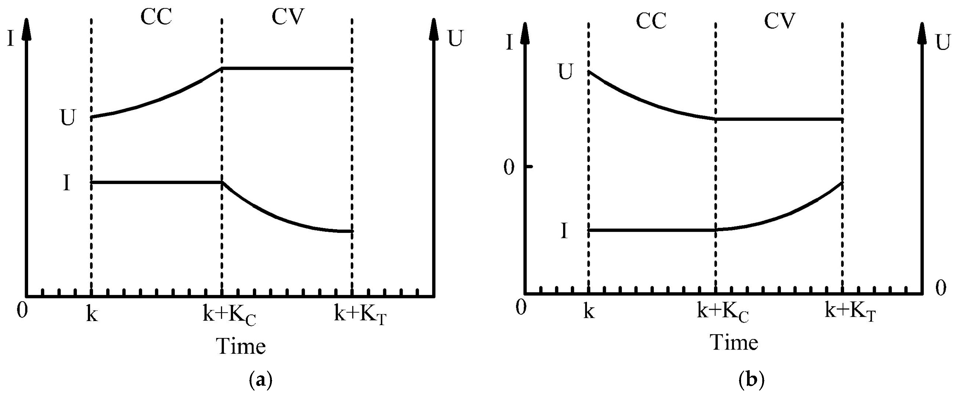
To predict the peak power, we should assume that during the prediction time horizon of peak power (i.e., seconds), the battery is under peak state condition. When the battery is working under peak state condition, the battery is in either constant current (CC) limit condition or constant voltage limit (CV) condition, as shown in Figure 3.
The battery voltage changes with battery current. Reviewing the battery model in Figure 1, we discover that when the battery is in charge under a constant current limit, the voltage gradually increases because the OCV increases and because of the continuity of the voltage over the ohmic resistors, and until the voltage limit. Then, the battery will be in charge under a constant voltage limit until the current reaches the margin. Similarly when the battery is in discharge under a constant current limit, the voltage will gradually decrease until the voltage limit; then, the battery will be in discharge under constant voltage limit until the current reaches the margin.
3.2. Rapid-Calculating Peak Power/SOP Method
Assume during the peak power prediction time horizon seconds that the constant current process lasts for seconds and the constant voltage process lasts for seconds. Corresponding to the sampling time , seconds contains sampling points, seconds contains sampling points, and seconds contains sampling points.
3.2.1. Traditional Peak Power/SOP Method
According to the introduction above, the traditional peak power during time horizon seconds can be described as follows: based on the battery states and parameters at moment, calculate the product of the current and the voltage from the moment to the moment in peak state; then, among the product values, the product value close to zero represents the peak power during time horizon seconds.
3.2.2. Rapid-Calculating Peak Power/SOP Method
According to Figure 3, the charge peak power during seconds only needs to work out the minimum between the peak power at the moment and the peak power at the moment; and the discharge peak power during seconds only needs to work out the maximum between peak power at the moment and peak power at the moment, that is, the discharge peak power during seconds is the peak power at the moment.
3.3. Single Constraint
In this section, the peak power under a single constraint—including designed power constraint, current constraint, SOC constraint, and voltage constraint—will be discussed.
3.3.1. Designed Power Constraint
The battery peak power must satisfy the designed battery power constraint shown in Equation (27):
3.3.2. Current Constraint
Assume that the battery works under the battery-designed constant current in the whole prediction time horizon; that is, the current , the system excitation , where , and especially in charge peak state and in discharge peak state. To calculate the peak power, the terminal voltage must be predicted.
Rewrite Equation (6) as Equations (28) and (29):
According to Equation (28), the state vector and at the moment can be expressed as Equation (30). Substituting Equation (30) into Equation (29), Equation (31) can be deduced:
Therefore, according to the rapid-calculating method in Section 3.2, the peak power at the kth moment under the battery designed constant current can be expressed by Equations (32) and (33).
3.3.3. SOC Constraint
The peak power with SOC constraint was first proposed by Plett [20]. For the sake of protecting the battery, the SOC must have design limits: that is, . For a constant current in prediction time horizon , the SOC can be expressed as Equation (34):
Therefore, the maximum charge current and the minimum discharge current under SOC constraint can be calculated by Equations (35) and (36):
According to the rapid-calculating method in Section 3.2, the peak power at the kth moment under the SOC constraint can be expressed by Equations (37) and (38) and and can be calculated by Equation (31):
3.3.4. Voltage Constraint
Assume that the battery works under a constant voltage limit in the whole prediction time horizon ; that is, the voltage where .
Rewrite Equation (29) as Equation (39):
Substitute Equation (39) into Equation (28) to deduce Equation (40):
where and represent the first and second column of , respectively.
Equation (40) can be rewritten by iteration as Equation (41):
Substitute Equation (41) into Equation (39) to deduce Equation (42):
Therefore, according to the rapid-calculating method in Section 3.2, the peak power under voltage constraint can be expressed by Equations (43) and (44):
3.4. Multiple Constraints
The peak power in single-designed power, current, SOC, and voltage constraints has been discussed above. In this section, the peak power under multiple constraints of current, voltage, SOC, and power will be discussed.
3.4.1. Current and Voltage Dual-Constraint
The peak power in the hybrid current and voltage peak state will be determined in this part, assuming that the constant current peak state lasts for seconds (i.e., ) and the constant voltage peak state lasts for seconds (i.e., ).
Making replace in Equation (31), we can get the solution with the bisection method.
If , will not reach in the whole seconds time horizon; thus, .
If , the whole peak state will be constant current state first, then switches to constant voltage state; thus, , .
If , , the whole peak state will keep in constant voltage state; thus, .
In the whole peak state, the voltage and the current can be expressed by Equations (45) and (46). in Equation (46) can be expressed by Equation (47):
The peak power of every sampling time in the peak power state can be calculate by Equation (48). According to the rapid-calculating method proposed in Section 3.2, the peak power expression under dual current and voltage constraints of the whole peak power state can be obtained, as shown in Equations (49) and (50):
3.4.2. Multiple Constraints of Current, Voltage, SOC, and Power
Taking multiple constraints of current, voltage, SOC, and power into account, we can obtain the final peak power during prediction time horizon at the moment, as shown in Equations (51) and (52):
3.5. SOP Calculation
As the peak power of the battery has been obtained, the state-of-power can be calculated by Equations (53) and (54). represents the nominal power of the battery:
4. Experimental Design
4.1. Test Bench and Experiment Object
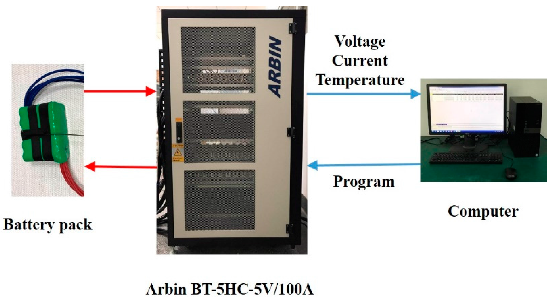
The test structure of the experimental system is shown in Figure 4, which consisted of an Arbin battery test system BT-5HC-5V/100 A, a battery pack, and a host computer. The test equipment BT-5HC-5V/100 A had 3 scales (100 A/10 A/1 A) and its operating voltage was 0–5 V. The resolution of the current and voltage was .
A battery pack consisting of 10 Panasonic NCR18650PF lithium ion batteries was chosen for the test. The designed parameters of NCR18650PF battery are shown in Table 1. The battery pack in this experiment had a nominal capacity of 26.6 Ah and its maximum charge and minimum discharge power were 250 W and −320 W, respectively. The designed upper and lower bounds of its voltage were 4.2 V and 2.5 V, respectively, and the charge and discharge bounds of its current were 2 C and −3 C, respectively. The C-rate is defined as the ratio of battery operation current to the manufacturer’s rated capacity (in ampere-hours) [19]. Briefly speaking, in this paper, 1 C corresponds to 26.6 A.
4.2. Experimental Procedure
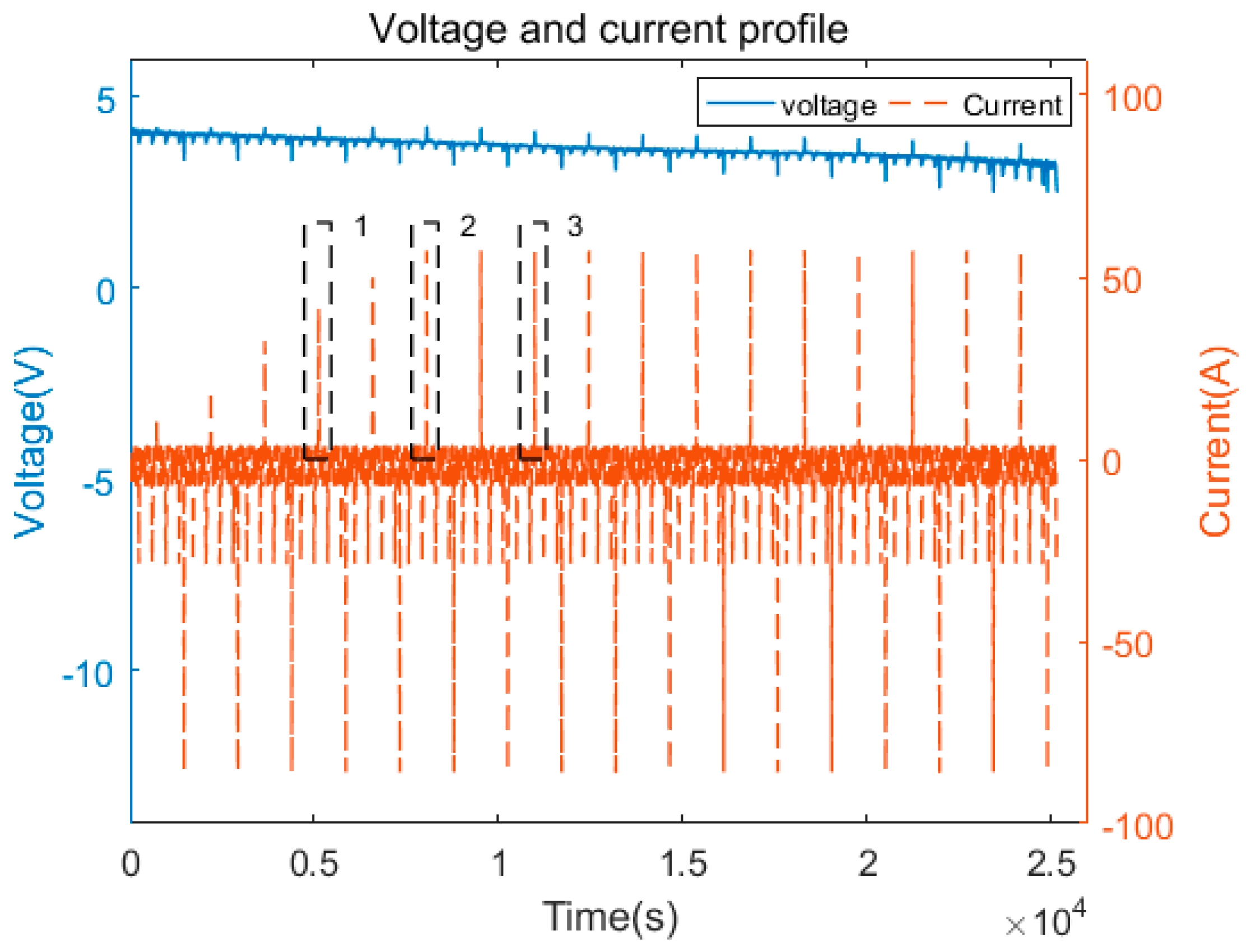
In order to verify the novel SOP estimation algorithm, a simplified version of the Federal Urban Driving Schedule (SFUDS) with an inserted pulse experiment was conducted. The operational voltage and current profile are depicted in Figure 5.
It can be noticed that the maximum constant charge current (2 C) pulses and minimum discharge constant current (−3 C) pulses were added to the profile to measure the true peak power of the battery pack. If the battery pack terminal voltage reaches the voltage limit in the constant pulse, the battery pack will operate at constant voltage. During the operation, the charge current pulses and the discharge current pulses were inserted every two SFUDS cycles.
Experiments of three sets of SFUDS with a 10 s pulse, a 20 s pulse, and a 30 s pulse were conducted. The close-to-zero values of the power measured in the pulses are regarded as the true peak power of the battery pack.
5. Verification and Discussion
5.1. Verification for Battery Model
According to the DEKF-based parameters and state estimations, the battery pack terminal voltage can be calculated. In Figure 6, the results of the battery terminal voltage obtained based on DEKF simulation and the battery terminal voltage obtained based on the experimental test with a 10 s pulse are compared. The RMSE of the terminal voltage is 0.037 V, which indicates the battery with the DEKF-based parameters and states had good accuracy.
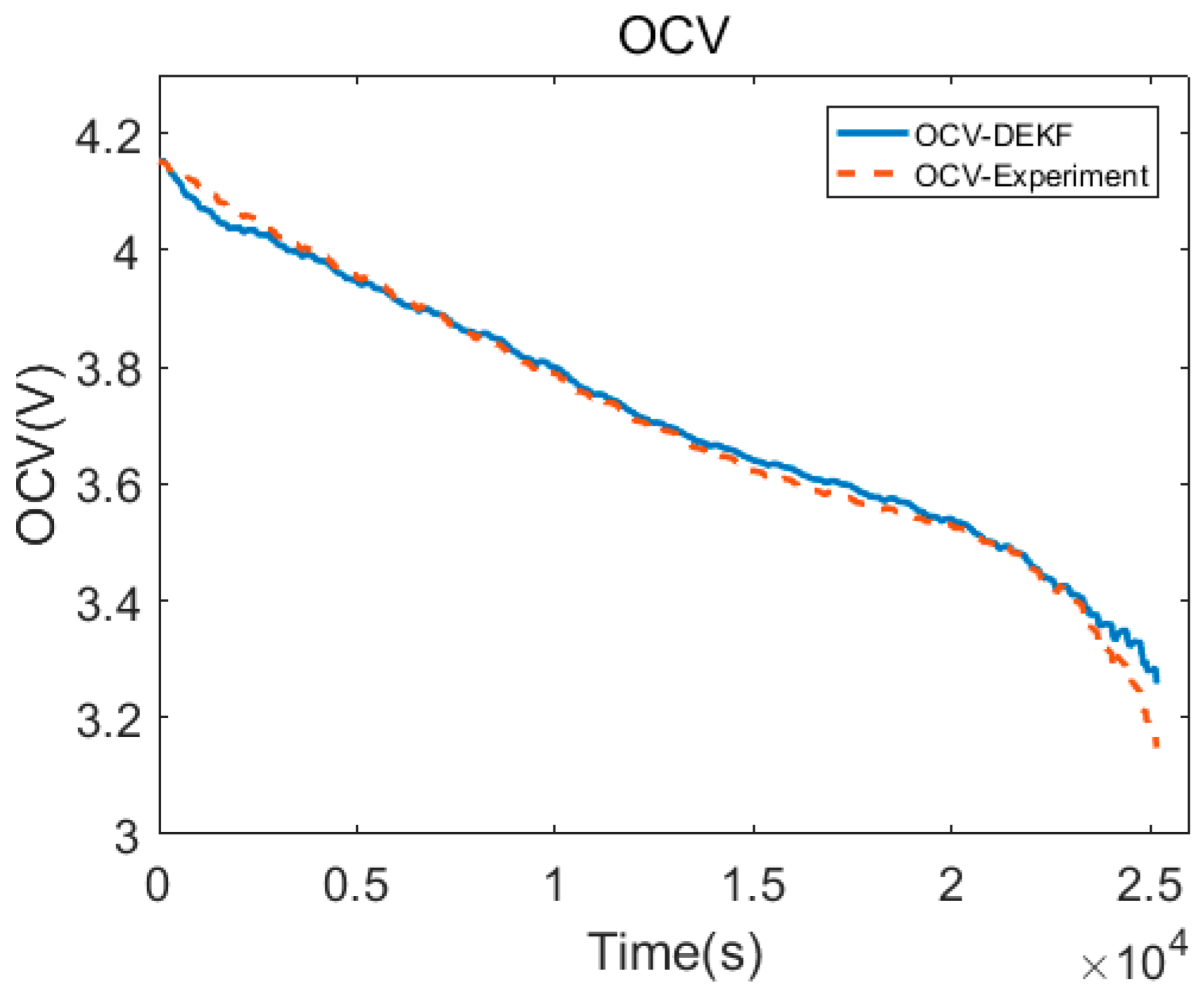
5.2. Verification for the DEKF-Based OCV Estimation
The results of the OCV obtained based on DEKF simulation and the OCV obtained based on offline experimental tests are compared in Figure 7, which shows the RMSE of OCV is 0.0218 V. As shown in Figure 7, by the end of the experiment, the error is relatively large because the real OCV changes fast in that stage; however, the process noise covariance in Section 2.2.1 was set as a constant value in the whole operating process. This does not have an enormous impact on the state estimation owing to the fact that HEVs, PHEVs, and BEVs barely operate in such a SOC range.
5.3. Verification for the SOC Estimation
According to the OCV based on DEKF, we can calculate the SOC by using the offline measured OCV-SOC relationship, which is called the OCV method. In addition, the SOC was estimated with the DEKF method given in Section 2.2.2.
The SOC estimation result based on the OCV method and the DEKF method are compared with the true SOC shown in Figure 8. The results indicate that although the estimation of SOC based on the OCV method has an accuracy of 1.98% in RMSE, the estimation based on the DEKF method has a higher accuracy of 0.28% in RMSE.
5.4. Verification of the Peak Power and SOP Estimation
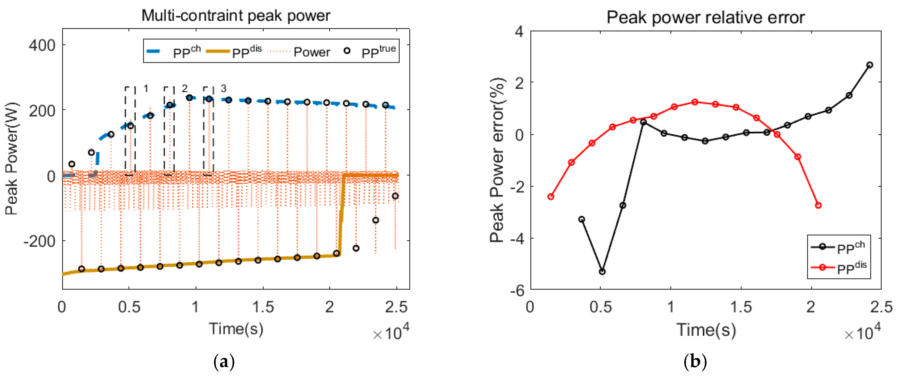
In what follows, we assume that and . The peak power estimation result has been plotted in Figure 9a. The orange dotted lines represent the actual power at every sampling point and the blue dotted line and the yellow solid line represent the estimated charge peak power in 10 s and the estimated discharge peak power in 10 s, respectively. Finally, the black circles represent the true peak power in the pulse of 10 s.
Both the estimated charge and the discharge peak power curves go through the black circles nicely. The relative error between the estimated peak power and the measured peak power is shown in Figure 9b.
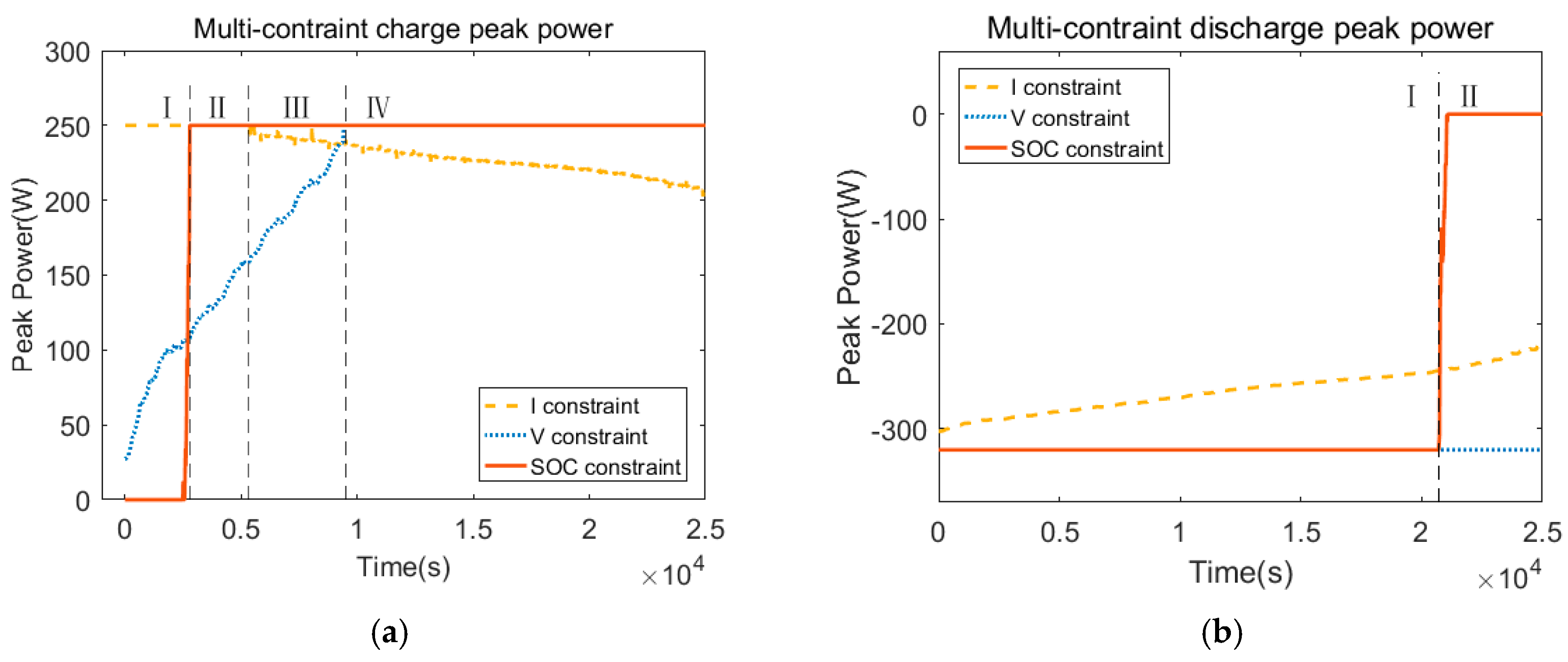
Figure 10a,b represent the charge and discharge peak power, respectively, under multiple constraints of current, voltage, SOC, and designed power. If the peak power under multiple constraints runs over the designed power constraint, we stipulate that the peak power is equal to the designed power.
As shown in Figure 10a segment Ι, the current calculated by Equation (35) increases from zero; therefore, the peak power under the SOC constraint is the minimum. In segment ΙΙ, the battery operates in constant voltage peak state at all times so the voltage constraint plays a decisive role. In segment ΙΙΙ, the battery reaches the constant current peak state first and then converts to constant voltage peak state; the current and voltage constraints jointly limit the peak power. In segment ΙV, the battery operates in constant current peak state at all times and the current constraint plays a decisive role.
As shown in Figure 10b segment Ι, the battery operates in constant current peak state at all times so the current constraint plays a decisive role. Then, the battery SOC gradually reaches its limit. Hence, in segment ΙΙ the battery peak power is under SOC constraint.
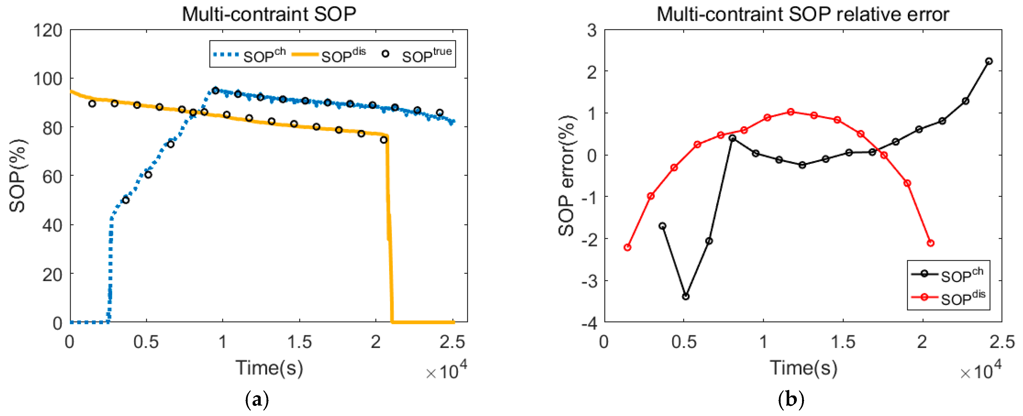
Based on Equations (53) and (54), the results of SOP estimation and relative error results are shown in Figure 11a,b, respectively.
5.5. Verification of the Rapid-Calculating Method
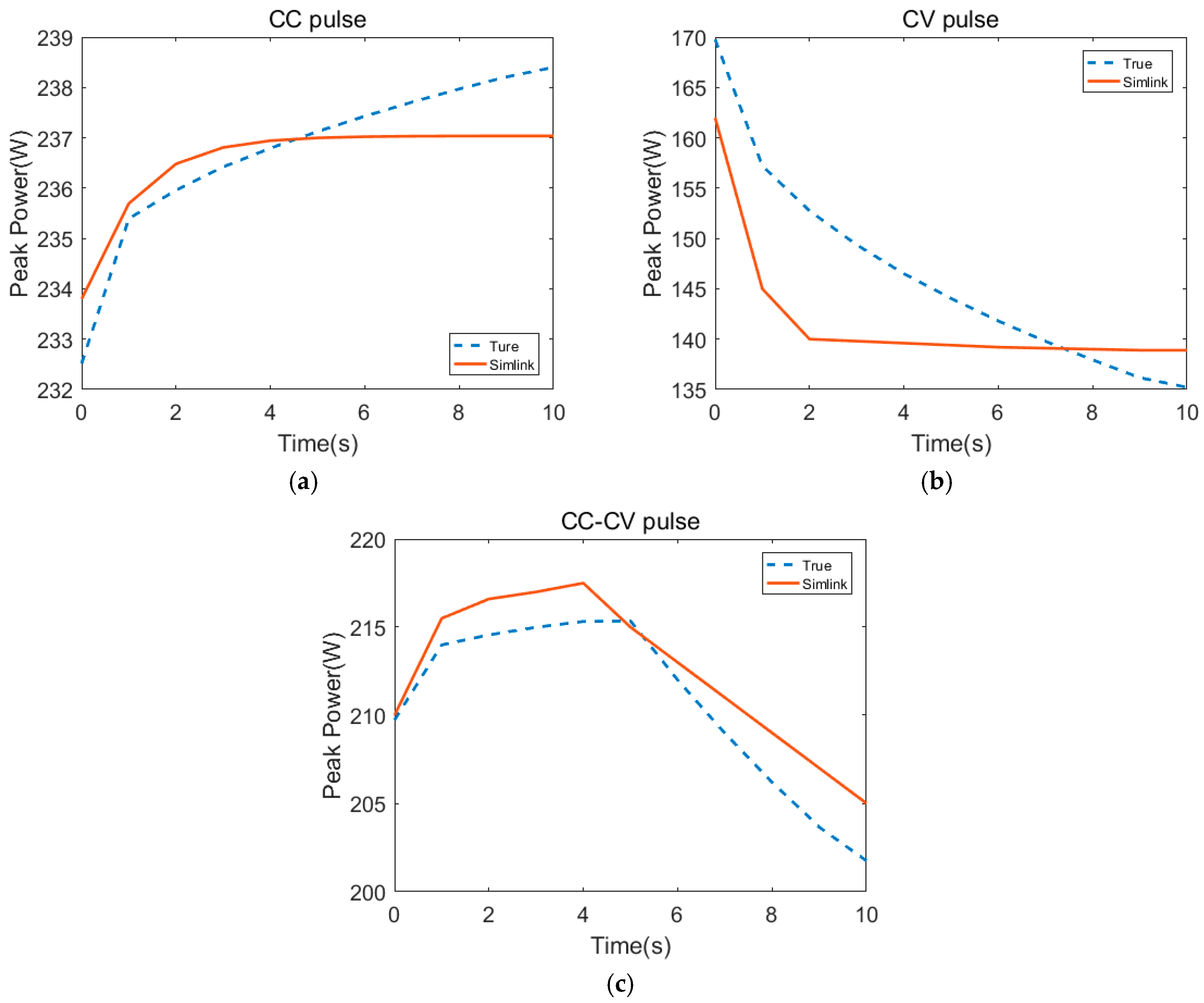
As shown in Figure 5, three typical charge pulses 1, 2, 3 corresponding to the CV pulse, CC-CV pulse, and CC pulse, respectively, were chosen to analyze in Figure 12. In the CC pulse, both the experimental power and the estimated power increase gradually and the power at the initial moment is the minimum power (i.e., peak power in the CC pulse). In the CV pulse, both the experimental power and the estimated power decrease gradually and the power at the last moment is the minimum power (i.e., peak power in CV pulse).
In the CC-CV pulse, both the experimental power and the estimated power increase first and then decrease; the smaller one of the power at the initial moment and the power at the last moment is the minimum power (i.e., peak power in CC-CV pulse). Based on the above analysis, the method that calculates peak power during seconds through one or two instantaneous peak powers proposed in Section 3.2 is proven to be effective.
For further verification, the rapid-calculating peak power/SOP method (RCM) is compared with the traditional method (TRM) in terms of accuracy and calculation time (Table 2). Analyzing Table 2, we can draw the following conclusions: (1) The RCM has the same accuracy as TRM; (2) The RCM has a significant improvement in terms of calculation efficiency; (3) As the prediction time horizon increases from 10 s to 30 s, the ratio of the RCM calculation time to TRM calculation time sharply decreases from 71.1% to 23.5%, which indicates the RCM has an increasing advantage in terms of calculation time; (4) As the prediction time horizon increases from 10 s to 30 s, the estimated RMSE gradually increases.
6. Conclusions
This article firstly introduced the definition and current research status of peak power/SOP. Then, based on the improved first-order RC model with one-state hysteresis, and using the DEKF method, the battery parameters and states including OCV were estimated. Furthermore, by employing the estimated OCV as the observed value to build the second dual Kalman filters, the battery SOC was estimated. In particular, the rapid-calculating estimation method of peak power/SOP under single constraint and multiple constraints was explored. Finally, the estimation method of OCV, SOC, and peak power/SOP was verified, and the actual constraint of a battery was analyzed specifically. Three conclusions can be drawn as follows:
- (1).
- The improved first-order RC model with one-state hysteresis and with parameters estimated online by DEKF has a high accuracy of 0.037 V in RMSE, which confirms the accuracy of the battery model to estimate SOC and peak power/SOP.
- (2).
- The DEKF-based OCV estimation has an RMSE of 0.0218 V and using the OCV estimated as the observed value, the SOC based on DEKF has a smaller RMSE of 0.28% than the one of 1.98% based on the OCV-SOC look-up method.
- (3).
- The peak power/SOP estimated under multiple constraints has the maximum relative error 6%/4%. The proposed rapid-calculating peak power method in Section 3.2 that calculates peak power during seconds through one or two instantaneous peak power is proven to be more effective.
Acknowledgments
This research was supported by Sichuan Plug-in Hybrid Logistics Vehicle Research Project (Grant No. 2016GZ0024), Sichuan Talent Research Project (Grant No. 2016RZ0043), Sichuan New Energy Vehicles Control and Key Technologies of Power Battery Management System Project (Grant No. 2015JY0281), Sichuan Major Scientific and Technological Achievements Transformation Project (Grant No. 2015CC0003), and SWJTU Graduate Innovative Experimental Practice Program (Grant No. YC201502109). The authors also thank the reviewers for their corrections and helpful suggestions.
Author Contributions
Shun Xiang, Guangdi Hu and Ruisen Huang proposed the idea based on the research status, and accomplished the first draft; Shun Xiang, Ruisen Huang and Feng Guo conceived and designed the experiments; Pengkai Zhou and Feng Guo conducted the experiments and analyzed data; Shun Xiang, Ruisen Huang, and Guangdi Hu revised the paper.
Conflicts of Interest
The authors declare no conflict of interest.
Nomenclature
| Symbols | |
| Simulink time, s | |
| prediction time horizon of peak power, s | |
| sampling time, s | |
| load current, A | |
| terminal voltage, V | |
| open-circuit voltage, V | |
| hysteresis voltage, V | |
| voltage across , V | |
| ohmic resistance, Ω | |
| charge ohmic resistance, Ω | |
| discharge ohmic resistance, Ω | |
| diffusion capacitance, F | |
| diffusion resistance, Ω | |
| maximum polarization due to hysteresis, V | |
| rate of decay | |
| sign function of | |
| battery nominal capacity, Ah | |
| coulombic efficiency | |
| time constant of a parallel resistance-capacitance circuit, s | |
| time of constant current (voltage) process, s | |
| total number of sampling points in | |
| peak power, W | |
| battery power design limit, W | |
| battery current design limit, A | |
| battery voltage design limit, V | |
| nominal power, W | |
| Subscripts, Superscripts | |
| time step index | |
| ch | charge |
| dis | discharge |
| max | upper limit value |
| min | lower limit value |
| - | estimation value |
| + | posteriori estimation value |
| Abbreviations | |
| BEV | battery electric vehicle |
| BMS | battery management system |
| CC | constant current |
| CV | constant voltage |
| DEKF | dual extended Kalman filtering |
| HEV | hybrid electric vehicle |
| HPPC | hybrid pulse power characterization |
| OCV | open-circuit voltage |
| PHEV | plug-in hybrid electric vehicle |
| PNGV | Partnership for New Generation Vehicle |
| RC | resistance-capacitance |
| RCM | rapid-calculating method |
| RMSE | root mean square error |
| SFUDS | Simplified version of the Federal Urban Driving Schedule |
| SOC | state of charge |
| SOH | state of health |
| SOP | state of power |
| TRM | traditional method |
References
- Chu, S.; Majumdar, A. Opportunities and challenges for a sustainable energy future. Nature 2012, 488, 294–303. [Google Scholar] [CrossRef] [PubMed]
- Un-Noor, F.; Padmanaban, S.; Mihet-Popa, L.; Mollah, M.N.; Hossain, E.; Sciubba, E. A Comprehensive Study of Key Electric Vehicle (EV) Components, Technologies, Challenges, Impacts, and Future Direction of Development. Energies 2017, 10, 1217. [Google Scholar] [CrossRef]
- Andwari, A.M.; Pesiridis, A.; Rajoo, S.; Martinez-Botas, R.; Esfahanian, V. A review of Battery Electric Vehicle technology and readiness levels. Renew. Sustain. Energy Rev. 2017, 78, 414–430. [Google Scholar] [CrossRef]
- Pollet, B.G.; Staffell, I.; Shang, J.L. Current status of hybrid, battery and fuel cell electric vehicles: From electrochemistry to market prospects. Electrochim. Acta 2012, 84, 235–249. [Google Scholar] [CrossRef]
- Hannan, M.A.; Azidin, F.A.; Mohamed, A. Hybrid electric vehicles and their challenges: A review. Renew. Sustain. Energy Rev. 2014, 29, 135–150. [Google Scholar] [CrossRef]
- Lu, L.; Han, X.; Li, J.; Hua, J.; Ouyang, M. A review on the key issues for lithium-ion battery management in electric vehicles. J. Power Sources 2013, 226, 272–288. [Google Scholar] [CrossRef]
- Rahimi-Eichi, H.; Ojha, U.; Baronti, F.; Chow, M. Battery Management System: An Overview of Its Application in the Smart Grid and Electric Vehicles. IEEE Ind. Electron. Mag. 2013, 7, 4–16. [Google Scholar] [CrossRef]
- Xing, Y.; Ma, E.W.M.; Tsui, K.L.; Pecht, M. Battery Management Systems in Electric and Hybrid Vehicles. Energies 2011, 4, 1840–1857. [Google Scholar] [CrossRef]
- Hannan, M.A.; Lipu, M.S.H.; Hussain, A.; Mohamed, A. A review of lithium-ion battery state of charge estimation and management system in electric vehicle applications: Challenges and recommendations. Renew. Sustain. Energy Rev. 2017, 78, 834–854. [Google Scholar] [CrossRef]
- Gao, Z.; Cheng, S.C.; Chiew, J.H.K.; Jia, J.; Zhang, C. Design and Implementation of a Smart Lithium-Ion Battery System with Real-Time Fault Diagnosis Capability for Electric Vehicles. Energies 2017, 10, 1503. [Google Scholar] [CrossRef]
- Chiew, J.; Chin, C.; Jia, J.; Toh, W. Thermal Analysis of a Latent Heat Storage based Battery Thermal Cooling Wrap. In Proceedings of the 2017 COMSOL Conference—Call for Papers and Posters, Singapore, 9 March 2017. [Google Scholar]
- Panchal, S.; Mathewson, S.; Fraser, R.; Culham, R.; Fowler, M. Thermal Management of Lithium-Ion Pouch Cell with Indirect Liquid Cooling using Dual Cold Plates Approach. SAE Int. J. Altern. Powertrains 2015, 4, 293–307. [Google Scholar] [CrossRef]
- Nejad, S.; Gladwin, D.T.; Stone, D.A. A systematic review of lumped-parameter equivalent circuit models for real-time estimation of lithium-ion battery states. J. Power Sources 2016, 316, 183–196. [Google Scholar] [CrossRef]
- Berecibar, M.; Gandiaga, I.; Villarreal, I.; Omar, N.; Mierlo, J.V.; Bossche, P.V.D. Critical review of state of health estimation methods of Li-ion batteries for real applications. Renew. Sustain. Energy Rev. 2016, 56, 572–587. [Google Scholar] [CrossRef]
- Waag, W.; Fleischer, C.; Sauer, D.U. Critical review of the methods for monitoring of lithium-ion batteries in electric and hybrid vehicles. J. Power Sources 2014, 258, 321–339. [Google Scholar] [CrossRef]
- Plett, G.L. Extended Kalman filtering for battery management systems of LiPB-based HEV battery packs: Part 3. State and parameter estimation. J. Power Sources 2004, 134, 277–292. [Google Scholar] [CrossRef]
- Plett, G.L. Extended Kalman filtering for battery management systems of LiPB-based HEV battery packs: Part 2. Modeling and identification. J. Power Sources 2004, 134, 262–276. [Google Scholar] [CrossRef]
- Plett, G.L. Extended Kalman filtering for battery management systems of LiPB-based HEV battery packs: Part 1. Background. J. Power Sources 2004, 134, 252–261. [Google Scholar] [CrossRef]
- Idaho National Engineering & Environmental Laboratory. Battery Test Manual for Plug-In Hybrid Electric Vehicles; Assistant Secretary for Energy Efficiency and Renewable Energy (EE) Idaho Operations Office: Idaho Falls, ID, USA, 2010.
- Plett, G.L. High-performance battery-pack power estimation using a dynamic cell model. IEEE Trans. Veh. Technol. 2004, 53, 1586–1593. [Google Scholar] [CrossRef]
- Moura, S.J.; Chaturvedi, N.A.; Krstić, M. Adaptive Partial Differential Equation Observer for Battery State-of-Charge/State-of-Health Estimation Via an Electrochemical Model. J. Dyn. Syst. Meas. Control 2014, 136, 011015. [Google Scholar] [CrossRef]
- Hu, X.; Tang, X. Review of Modeling Techniques for Lithium-ion Traction Batteries in Electric Vehicles. J. Mech. Eng. 2017, 53, 20–31. [Google Scholar] [CrossRef]
- Hu, X.; Li, S.; Peng, H. A comparative study of equivalent circuit models for Li-ion batteries. J. Power Sources 2012, 198, 359–367. [Google Scholar] [CrossRef]
- Seaman, A.; Dao, T.S.; Mcphee, J. A survey of mathematics-based equivalent-circuit and electrochemical battery models for hybrid and electric vehicle simulation. J. Power Sources 2014, 256, 410–423. [Google Scholar] [CrossRef]
- Liu, C.; Liu, W.; Wang, L.; Hu, G.; Ma, L.; Ren, B. A new method of modeling and state of charge estimation of the battery. J. Power Sources 2016, 320, 1–12. [Google Scholar] [CrossRef]
- Dey, S.; Ayalew, B.; Pisu, P. Nonlinear Adaptive Observer for a Lithium-Ion Battery Cell Based on Coupled Electrochemical-Thermal Model. J. Dyn. Syst. Meas. Control 2015, 137, 111005. [Google Scholar] [CrossRef]
- Lin, X.; Perez, H.E.; Mohan, S.; Siegel, J.B.; Stefanopoulou, A.G.; Ding, Y.; Castanier, M.P. A lumped-parameter electro-thermal model for cylindrical batteries. J. Power Sources 2014, 257, 1–11. [Google Scholar] [CrossRef]
- Fotouhi, A.; Auger, D.J.; Propp, K.; Longo, S.; Wild, M. A review on electric vehicle battery modelling: From Lithium-ion toward Lithium–Sulphur. Renew. Sustain. Energy Rev. 2016, 56, 1008–1021. [Google Scholar] [CrossRef]
- Gao, Z.; Chin, C.S.; Woo, W.L.; Jia, J. Integrated Equivalent Circuit and Thermal Model for Simulation of Temperature-Dependent LiFePO4 Battery in Actual Embedded Application. Energies 2017, 10, 85. [Google Scholar] [CrossRef]
- Wang, J.; Liu, P.; Hicks-Garner, J.; Sherman, E.; Soukiazian, S.; Verbrugge, M.; Tataria, H.; Musser, J.; Finamore, P. Cycle-life model for graphite-LiFePO4 cells. J. Power Sources 2011, 196, 3942–3948. [Google Scholar] [CrossRef]
- Panchal, S.; Mcgrory, J.; Kong, J.; Fraser, R.; Fowler, M.; Dincer, I.; Agelin-Chaab, M. Cycling degradation testing and analysis of a LiFePO4 battery at actual conditions. Int. J. Energy Res. 2017, 41, 2565–2575. [Google Scholar] [CrossRef]
- Sun, F.; Xiong, R.; He, H.; Li, W.; Aussems, J.E.E. Model-based dynamic multi-parameter method for peak power estimation of lithium–ion batteries. Appl. Energy 2012, 96, 378–386. [Google Scholar] [CrossRef]
- Xiong, R.; He, H.; Sun, F.; Liu, X.; Liu, Z. Model-based state of charge and peak power capability joint estimation of lithium-ion battery in plug-in hybrid electric vehicles. J. Power Sources 2013, 229, 159–169. [Google Scholar] [CrossRef]
- Xiong, R.; Sun, F.; He, H.; Nguyen, T.D. A data-driven adaptive state of charge and power capability joint estimator of lithium-ion polymer battery used in electric vehicles. Energy 2013, 63, 295–308. [Google Scholar] [CrossRef]
- Pei, L.; Zhu, C.; Wang, T.; Lu, R.; Chan, C.C. Online peak power prediction based on a parameter and state estimator for lithium-ion batteries in electric vehicles. Energy 2014, 66, 766–778. [Google Scholar] [CrossRef]
- Sun, F.; Xiong, R.; He, H. Estimation of state-of-charge and state-of-power capability of lithium-ion battery considering varying health conditions. J. Power Sources 2014, 259, 166–176. [Google Scholar] [CrossRef]
- Feng, T.; Yang, L.; Zhao, X.; Zhang, H.; Qiang, J. Online identification of lithium-ion battery parameters based on an improved equivalent-circuit model and its implementation on battery state-of-power prediction. J. Power Sources 2015, 281, 192–203. [Google Scholar] [CrossRef]
- Zhang, W.; Shi, W.; Ma, Z. Adaptive unscented Kalman filter based state of energy and power capability estimation approach for lithium-ion battery. J. Power Sources 2015, 289, 50–62. [Google Scholar] [CrossRef]
- Jiang, J.; Liu, S.; Ma, Z.; Wang, L.Y.; Wu, K. Butler-Volmer equation-based model and its implementation on state of power prediction of high-power lithium titanate batteries considering temperature effects. Energy 2016, 117, 58–72. [Google Scholar] [CrossRef]
- Haykin, S.; Puskorius, G.V.; Feldkamp, L.A.; Patel, G.S.; Becker, S.; Racine, R.; Wan, E.A.; Nelson, A.T.; Roweis, S.T.; Ghahramani, Z.; et al. Dual Extended Kalman Filter Methods. In Kalman Filtering and Neural Networks; John Wiley & Sons, Inc.: Hoboken, NJ, USA, 2001; pp. 123–173. [Google Scholar]
- Cuma, M.U.; Koroglu, T. A comprehensive review on estimation strategies used in hybrid and battery electric vehicles. Renew. Sustain. Energy Rev. 2015, 42, 517–531. [Google Scholar] [CrossRef]
- He, H.; Zhang, X.; Xiong, R.; Xu, Y.; Guo, H. Online model-based estimation of state-of-charge and open-circuit voltage of lithium-ion batteries in electric vehicles. Energy 2012, 39, 310–318. [Google Scholar] [CrossRef]
- Zhang, J.; Lee, J. A review on prognostics and health monitoring of Li-ion battery. J. Power Sources 2011, 196, 6007–6014. [Google Scholar] [CrossRef]
Figure 1.
The improved first-order resistance-capacitance model with one-state hysteresis.
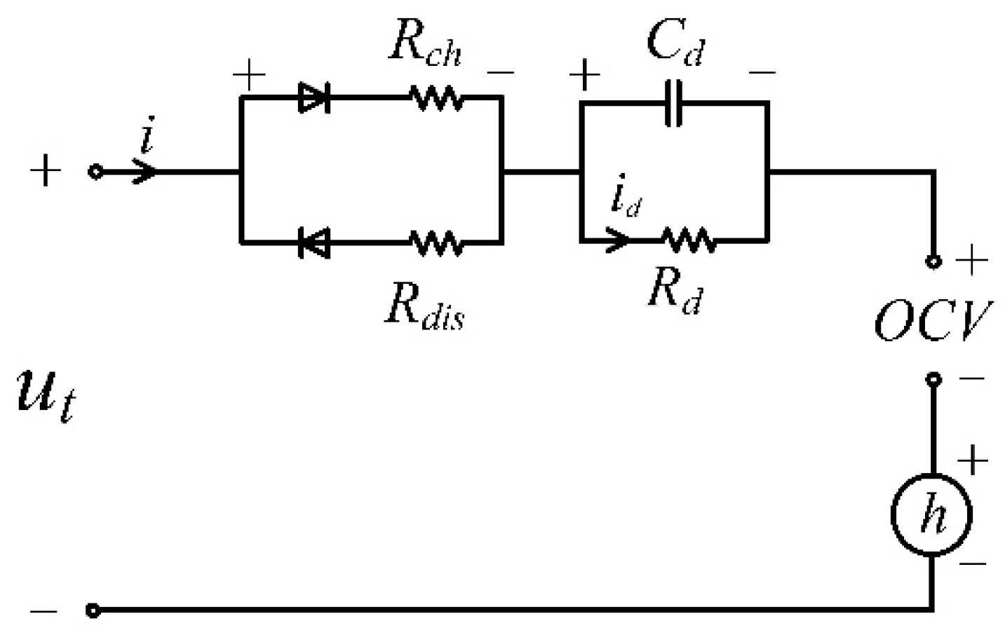
Figure 2.
The dual extended Kalman filtering algorithm.
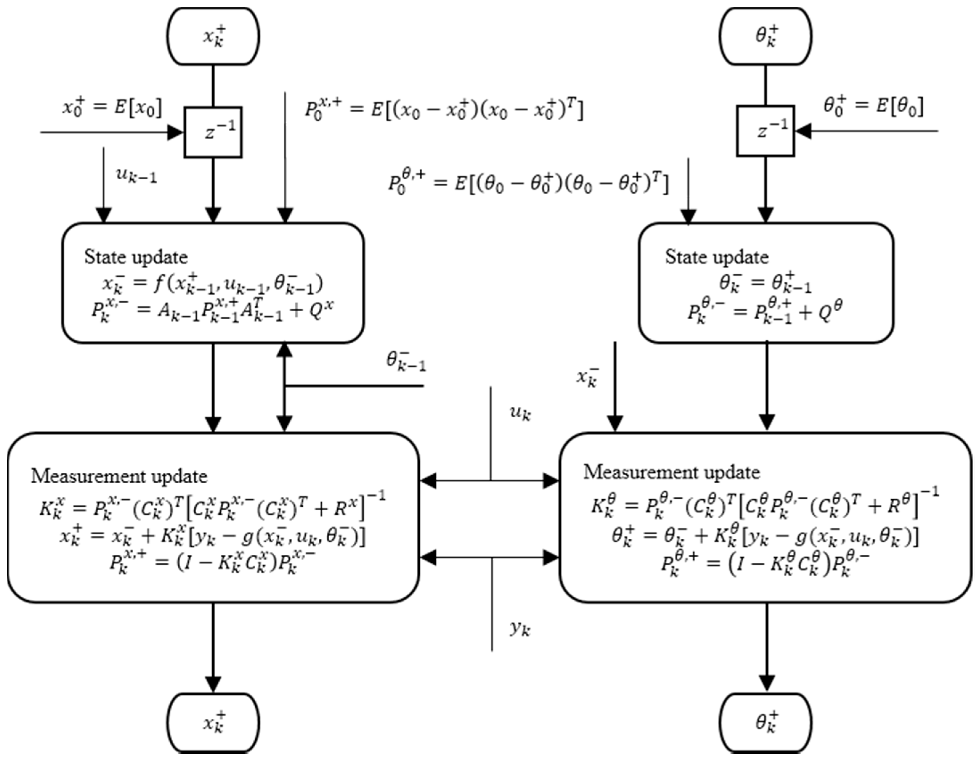
Figure 3.
Peak state: (a) Charge peak state; (b) Discharge peak state.

Figure 4.
Test bench.

Figure 5.
The operational voltage and current profile under the Federal Urban Driving Schedule (SFUDS).
Figure 5.
The operational voltage and current profile under the Federal Urban Driving Schedule (SFUDS).

Figure 6.
Comparison between simulated voltage and true voltage.
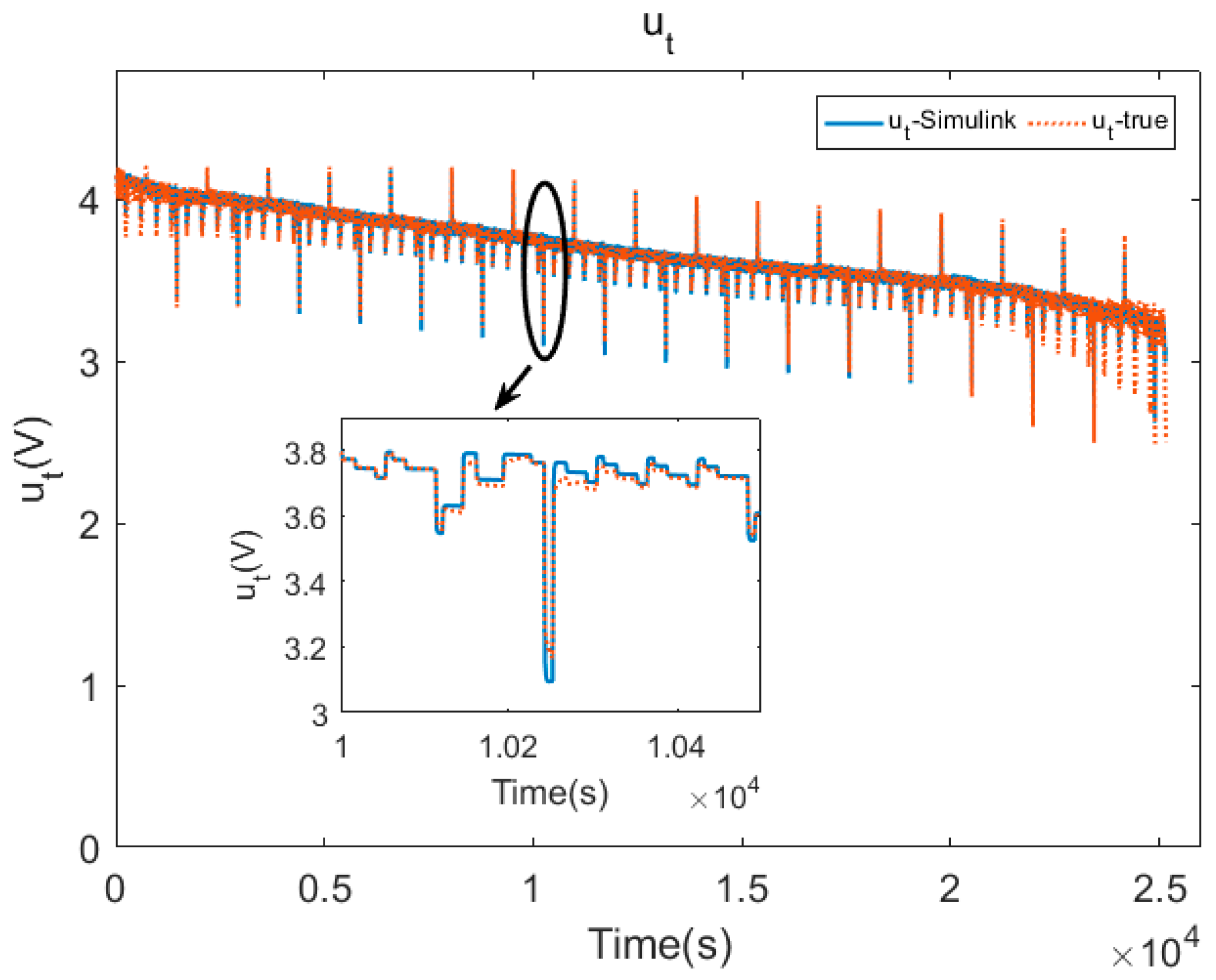
Figure 7.
Comparison between the open-circuit voltage (OCV) based on dual extended Kalman filtering (DEKF) simulation and OCV experimental tests.
Figure 7.
Comparison between the open-circuit voltage (OCV) based on dual extended Kalman filtering (DEKF) simulation and OCV experimental tests.

Figure 8.
Comparison of SOC-DEKF, SOC-Lookup, and SOC-True.
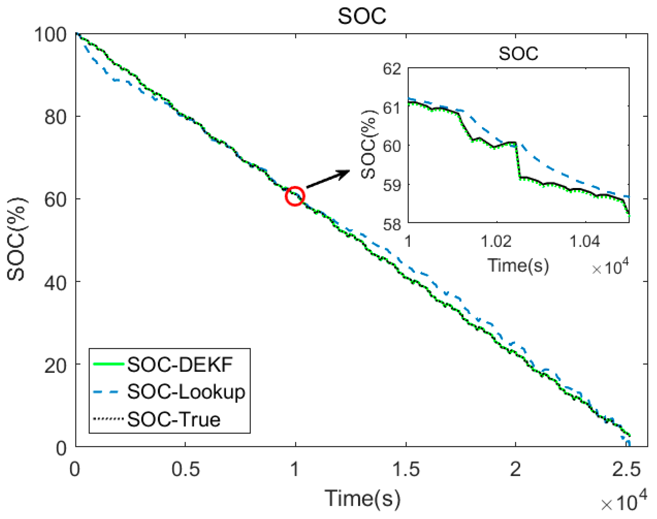
Figure 9.
(a) Peak power under multiple constraints; (b) Peak power relative errors.

Figure 10.
Battery peak power under multiple constraints: (a) charge peak power; (b) discharge peak power.
Figure 10.
Battery peak power under multiple constraints: (a) charge peak power; (b) discharge peak power.

Figure 11.
(a) SOP under multiple constraints; (b) Relative errors.

Figure 12.
Pulse peak power: (a) CC pulse; (b) CV pulse; (c) CC-CV pulse.

Table 1.
The designed parameters of NCR18650PF battery.
| Battery Parameters | Value |
|---|---|
| Anode material | MnO2 |
| Cathode material | Li |
| (Ah) | 26.6 |
| (A) | 53.2 |
| (A) | −79.8 |
| (V) | 4.2 |
| (V) | 2.5 |
| (W) | 250 |
| (W) | −320 |
| 0.2 | |
| 0.9 |
Table 2.
The comparison between the rapid-calculating method (RCM) and the traditional method (TRM).
Table 2.
The comparison between the rapid-calculating method (RCM) and the traditional method (TRM).
| PPch_RMSE (W) | PPdis_RMSE (W) | SOPch_RMSE (%) | SOPdis_RMSE (%) | Time (s) | tRCM/tTRM (%) | |
|---|---|---|---|---|---|---|
| Pulse_10s_RCM | 3.095 | 3.330 | 1.2 | 1.0 | 7.402 | 71.1 |
| Pulse_10s_TRM | 3.095 | 3.330 | 1.2 | 1.0 | 10.409 | / |
| Pulse_20s_RCM | 6.070 | 4.497 | 2.4 | 1.4 | 8.784 | 38.2 |
| Pulse_20s_TRM | 6.070 | 4.497 | 2.4 | 1.4 | 23.014 | / |
| Pulse_30s_RCM | 8.351 | 5.505 | 3.3 | 1.7 | 10.801 | 23.5 |
| Pulse_30s_TRM | 8.351 | 5.505 | 3.3 | 1.7 | 45.876 | / |
© 2018 by the authors. Licensee MDPI, Basel, Switzerland. This article is an open access article distributed under the terms and conditions of the Creative Commons Attribution (CC BY) license (http://creativecommons.org/licenses/by/4.0/).
Share and Cite
MDPI and ACS Style
Xiang, S.; Hu, G.; Huang, R.; Guo, F.; Zhou, P. Lithium-Ion Battery Online Rapid State-of-Power Estimation under Multiple Constraints. Energies 2018, 11, 283. https://doi.org/10.3390/en11020283
AMA Style
Xiang S, Hu G, Huang R, Guo F, Zhou P. Lithium-Ion Battery Online Rapid State-of-Power Estimation under Multiple Constraints. Energies. 2018; 11(2):283. https://doi.org/10.3390/en11020283
Chicago/Turabian StyleXiang, Shun, Guangdi Hu, Ruisen Huang, Feng Guo, and Pengkai Zhou. 2018. "Lithium-Ion Battery Online Rapid State-of-Power Estimation under Multiple Constraints" Energies 11, no. 2: 283. https://doi.org/10.3390/en11020283
Note that from the first issue of 2016, this journal uses article numbers instead of page numbers. See further details here.