Improved Finite-Control-Set Model Predictive Control for Cascaded H-Bridge Inverters

School of Electrical and Electronics Engineering, Chung-Ang University, Seoul 06974, Korea
*
Author to whom correspondence should be addressed.
Energies 2018, 11(2), 355; https://doi.org/10.3390/en11020355
Submission received: 25 December 2017
/
Revised: 29 January 2018
/
Accepted: 31 January 2018
/
Published: 2 February 2018
(This article belongs to the Special Issue Emerging Power Electronics Technologies for Power Systems and Machine Drives)
Abstract
:In multilevel cascaded H-bridge (CHB) inverters, the number of voltage vectors generated by the inverter quickly increases with increasing voltage level. However, because the sampling period is short, it is difficult to consider all the vectors as the voltage level increases. This paper proposes a model predictive control algorithm with reduced computational complexity and fast dynamic response for CHB inverters. The proposed method presents a robust approach to interpret a next step as a steady or transient state by comparing an optimal voltage vector at a present step and a reference voltage vector at the next step. During steady state, only an optimal vector at a present step and its adjacent vectors are considered as a candidate-vector subset. On the other hand, this paper defines a new candidate vector subset for the transient state, which consists of more vectors than those in the subset used for the steady state for fast dynamic speed; however, the vectors are less than all the possible vectors generated by the CHB inverter, for calculation simplicity. In conclusion, the proposed method can reduce the computational complexity without significantly deteriorating the dynamic responses.
1. Introduction
Multilevel converters generally consist of power switch elements and DC voltage sources such as independent sources or capacitors, which enables the synthesization of output voltage waveforms with several steps. These multilevel converters have been widely used in medium-voltage high-power industry because of their superior performance that includes a higher quality of output waveforms and a lower switching frequency compared to the two-level converters [1,2,3,4,5,6]. The multilevel converters are commonly classified into Neutral Point Clamped (NPC), Flying Capacitor (FC), and Cascaded H-bridge (CHB) converters [7,8,9]. Among them, the CHB types, which are based on a modular structure with isolated dc sources, do not require an increased number of clamping diodes and capacitors, each of which needs voltage balance control, as the voltage level is increased. In comparison with the other multilevel converters, because of the advantage of the CHB converters’ modularity, they are relatively simple to construct with high level of voltages [10,11,12]. Regarding the control issues of the CHB converters, linear proportional and integral controllers combined with multicarrier-based pulse-width modulation (PWM) schemes, such as the level-shift and phase-shift methods, have been extensively studied [13,14]. Besides the traditional linear control algorithms along with the PWM methods, studies on the finite-control-set model predictive control (FCS-MPC) methods, that can be simply implemented by removing the PWM block, have been properly conducted, given that the computational capability of the controllers has been improved as a result of the recent development of microprocessors [15,16,17,18]. The FCS-MPC algorithm predicts all possible next step trajectories of the control targets dependent on all possible switching states which the CHB converters can produce. Those predicted future values are compared with the reference values to select an optimum switching state. This straightforward FCS-MPC approach, which takes advantage of the inherently discrete nature of the converter switching actions, has several advantages, such as fast transient response, easy addition of constraints to the controller, and simple implementation through the removal of the PWM blocks. Owing to these advantages, the FCS-MPC methods have been widely applied for controlling the NPC, FC, and CHB multilevel converters [19]. The FCS-MPC method for the CHB converter [20,21] and inverter [22] calculates all the resulting voltage vectors from all the possible switching states to regulate the load currents of the converters. This basic principle of the FCS-MPC method, which predicts the next step behaviors using all possible voltage vectors, results in a problem of computational complexity for multilevel converters with a high number of voltage levels. This computational burden is a drawback for the CHB converters that are more accustomed to high voltage levels because the number of voltage vectors which the converter must generate increases quickly in proportion to the increased voltage level [20,21,22]. Because of a short sampling period, it is difficult to consider every voltage vector while attempting to determine an optimal switching state in the CHB converters with a high voltage level. In addition to the load current control block, external control algorithms such as speed controls and torque controls are added in the drive systems with the CHB converters which occupies a considerable calculation amount in general [23]. As a result, it can be necessary to reduce the calculation amount without significantly deteriorating other performances. In [22], a FCS-MPC method for CHB inverters with a reduced computational load is proposed. This method considers only seven vectors nearest to a present optimal vector to determine an optimal vector at the next step. In comparison with the conventional method, while considering all possible vectors, this approach can considerably reduce the level of computational complexity because it takes into account only seven vectors, similar to the two-level converters, regardless of the voltage level. However, when transient states occur, this method requires more steps to track the reference values by considering only the neighboring vectors, thus resulting in a slower dynamic response than the conventional method, while using all possible vectors.
This paper proposes an FCS-MPC algorithm with reduced computational complexity and fast dynamic response for CHB inverters, in which different candidate vector subsets to search for an optimal voltage vector are developed for the respective steady and transient states. The proposed method presents a robust approach for describing a next step as a steady or transient state by comparing an optimal voltage vector at a present step and a reference voltage vector at the next step. Because the proposed determinant algorithm is based on voltage vectors determined in the αβ plane, the distinction between steady state and transient state is free from switching ripple components and noise. During steady state, only an optimal vector at a present step and its adjacent vectors are considered as a candidate-vector subset. On the other hand, this paper defines a new candidate vector subset for the transient state, which consists of more vectors than those in the subset used for the steady state for fast dynamic speed, but of less vectors than all the possible vectors generated by the CHB inverter for calculation simplicity. The proposed method determines an optimal vector during the transient state by utilizing the new subset, which results in an excellent transient response performance. The proposed method, compared to the conventional technique using all possible vectors, can reduce the computational complexity without significantly deteriorating the dynamic responses. The effectiveness of the proposed method is verified via simulations and experimental results with a five-level CHB inverter, and is subsequently compared with that of the conventional method to demonstrate the merits of the proposed method. This paper is structured as follows: the principle of the FCS-MPC method for CHB inverters along with previous studies is described in Section 2. In Section 3, the proposed FCS-MPC method for reduced computational load and fast dynamics is presented. The simulations and experimental results of the conventional and proposed methods using a five-level CHB inverter are shown and compared in Section 4. The conclusions of this paper are then given in Section 5.
2. Conventional Finite-Control-Set Model Predictive Control Methods for Multilevel CHB Inverters
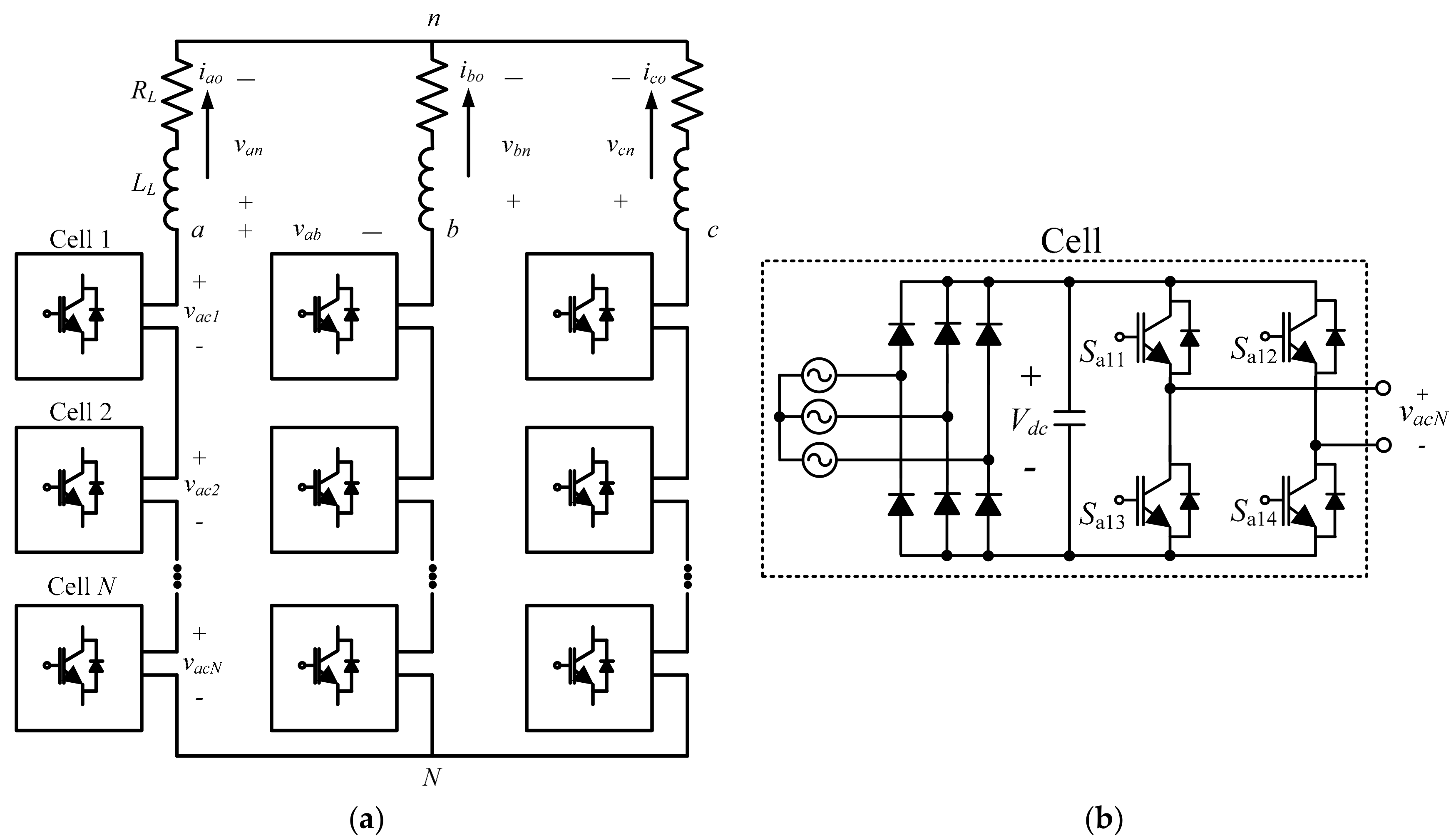
The multilevel CHB inverter is based on a series-connected structure as illustrated in Figure 1a. A single module used in the CHB inverter in Figure 1b consists of a single-phase two-level full bridge inverter with four switches. Each module is supplied with a DC voltage of equal magnitude as the individual power supply. Since each module consists of a two-level full bridge inverter, the output voltage of the module, vacx (x = 1, 2, ..., N), can be one of {Vdc, 0, −Vdc}. Consequently, the output voltage of each phase, viN (i = a, b, c), can be expressed as the sum of the output voltages of each module.
where, N is the number of series-connected H-bridge inverter cells per phase. The relationship of the total number of voltage vectors including the redundant voltage vectors, Lv, of the multilevel CHB inverter with the number of modules is expressed as
The total number of the switching states, SN, is expressed with the voltage vectors, Lv, which dramatically increases with increasing voltage level, as
Using the Kirchhoff voltage law in Figure 1, the three-phase inverter voltage (vaN, vbN, vcN) can be calculated as
where, RL, LL, and iio (i = a, b, c) denote the load resistance, load inductance, and load current at a, b, and c phases, respectively. Assuming three-phase balanced sinusoidal load currents, the common-mode voltage (vnN) shown in Equation (4) can be calculated as
The relationship of the inverter output, load, and the common-mode voltages can be written as
The three-phase load voltage can be simplified with a vector notation as
where, ,
In this paper, the simple Euler method is used to develop the discrete time model, and dio/dt can be expressed as follows, using a constant sampling period Ts.
By using the αβ transformation and substituting Equation (8), Equation (7) in the continuous abc frame can be represented in the discrete αβ frame as
where, . In addition, and , and represent the α and β components of one-step future current and present-current vectors, respectively. Furthermore, and represent the α and β component voltage values, which can be applied at a present step, respectively.
Predicting one-step future currents can be obtained through the possible voltage vectors of the CHB multilevel inverter, as shown in Equation (9). Thus, as the output voltage level of the CHB inverter increases, the total number of one-step predicted current values greatly increases. The conventional FCS-MPC method (termed as MPC-conv1 in this paper) considers all predicted currents generated by all possible voltage vectors to determine an optimal voltage vector at the next step [20,21,22]. Therefore, as the level increases, the calculation complexity of the MPC-conv1 method is increased. The cost function, h, defined using Equation (10), can be used to determine an optimal vector leading to the smallest error values between the reference and the predicted current values.
where, and represent the α and β components of the reference current vector at the next step, respectively.
Using Lagrange extrapolation, the one-step future reference current can be calculated for the cost function in Equation (10) as
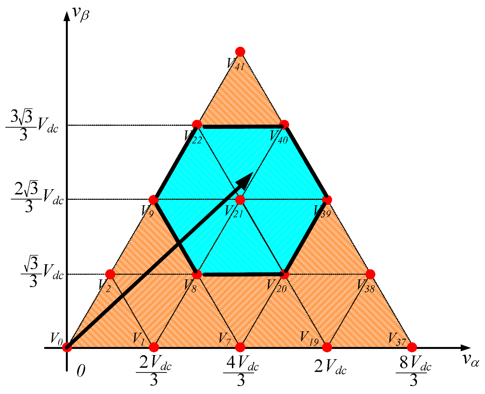
Figure 2 shows the voltage vector diagram of the multilevel CHB inverter with M-level, in which the number of redundant voltage vectors are included. It can be seen that the outer voltage vectors possess less redundant voltage vectors than their inner counterparts. When the voltage level increases in the multilevel CHB inverter, the number of voltage vectors and the number of the redundant voltage vectors quickly increases as well. In order to reduce the redundant vector state in the CHB inverters, a voltage vector, which can minimize a common-mode voltage among numerous redundant vectors, is selected [22]. The number of non-redundant voltage vectors, Nnr, according to the voltage level, can be calculated as
Table 1 lists the number of voltage vectors and voltage levels according to the voltage level. Although the number of voltage vectors is reduced by eliminating the redundant vectors, as indicated in Table 1, the MPC-conv1 method considering all non-redundant voltage vectors generated by the multilevel CHB inverter still suffers from a rapidly increased computational load as the voltage level increases. Therefore, the incorporation of a computational complexity reduction algorithm into the MPC-conv1 method is needed for the multilevel CHB inverter.
In steady state, the reference sinusoidal currents change slowly, and, correspondingly, an optimal voltage vector forcing the actual load currents to track the reference currents smoothly moves without sudden transitions. This implies that the optimal voltage vectors as well as the reference current vectors steadily rotate in the αβ plane. Thus, an optimal voltage vector at the next step is located near an optimal vector at the present step. On the basis of this fact, the FCS-MPC method was proposed, which selects a next-step optimal vector only among the neighboring vectors of a present optimal vector [22]. In this paper, this is referred to as the MPC-conv2 method, which uses a subset consisting of seven vectors near a present optimal voltage vector in the αβ plane, in the calculation process of the cost function. Compared to the MPC-conv1 method, the MPC-conv2 variant can greatly reduce the computational complexity by considering only the optimal vector of the previous step and its adjacent vectors. As a result, the total number of voltage vectors calculated to determine an optimal vector for every step in the cost function in Equation (10) is only seven, and this is regardless of the voltage level, which is exactly the same as the case of the two-level inverter. Figure 3 shows, in the αβ plane, the candidate voltage vectors used in the MPC-conv2 method in the case that an optimal voltage vector at present step is V21. In addition, the MPC-conv2 method can produce the same harmonic spectrum quality of load current waveforms as the MPC-conv1 method in steady state. However, despite the dramatically decreased calculation load, the MPC-conv2 method is more vulnerable to a slower transient response than the MPC-conv1 method. The MPC-conv2 method requires more steps to follow the step-change of the reference currents than the MPC-conv1 method when a transient state occurs. This is due to the limited candidate voltage vectors in the search process for an optimal vector.
3. Proposed Predictive Control Method for Single-Phase Inverter
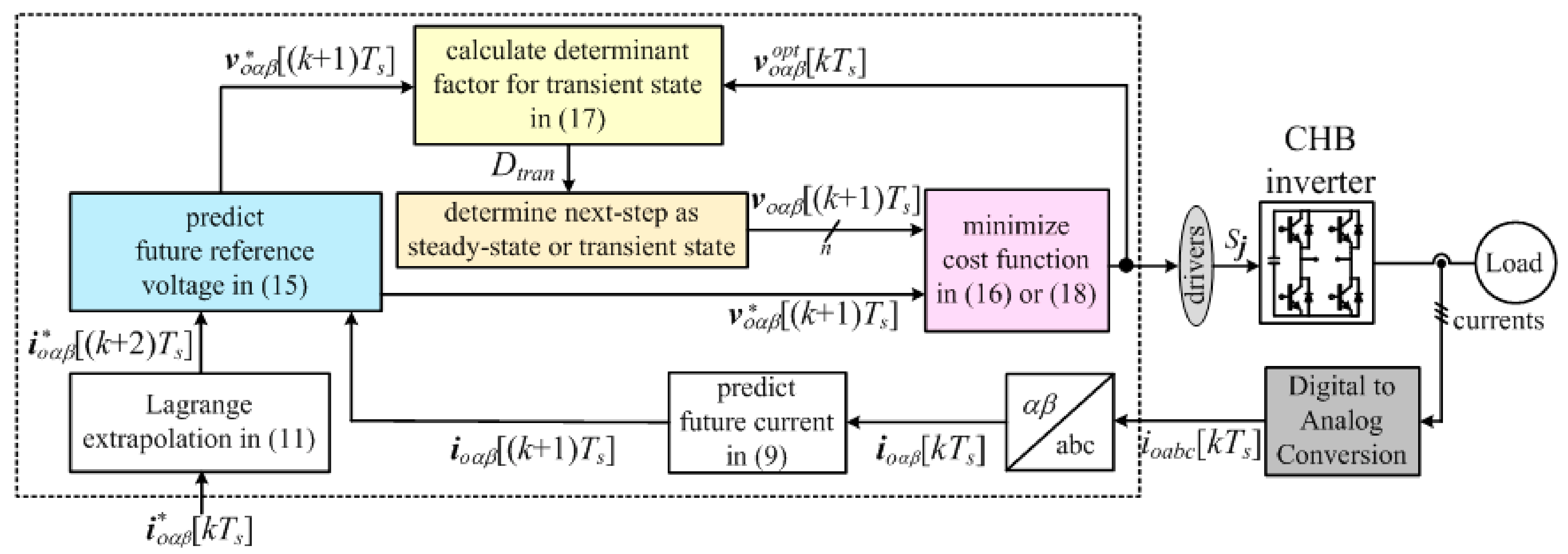
This paper proposes an FCS-MPC algorithm with reduced computational complexity and fast dynamic response for multilevel CHB inverters to effectively improve the computational load of the MPC-conv1 method and the slow dynamic response of the MPC-conv2 method. Figure 4 represents a block diagram of the proposed FCS-MPC method for a multilevel CHB inverter. The proposed algorithm employs different candidate vector subsets to determine an optimal voltage vector for the steady and transient states, respectively. As a result, a distinction algorithm, which can categorize a next step as either steady or transient state, is developed in the proposed method. In order to develop the distinction algorithm to more clearly distinguish between steady and transient states, the proposed method utilizes predicted voltage vectors instead of the current vectors used in conventional methods.
The load dynamic equation (9) can be rewritten as the relationship between the voltages and the present and one-step future load currents
where, and . In addition, by assuming that the actual currents at the next step become equal to the reference current values by applying the reference voltage vector at the present step, the Equation (13) can be expressed as
where, and represent the α and β components of the reference voltage vector, respectively. The Equation (14) is shifted by one-step future to apply the delay compensation method, which is needed for the inevitable time delay of the controllers [24].
The reference voltage vector obtained using Equation (15) is compared using a cost function with the candidate voltage vectors to determine a future optimal voltage vector that enables a future load current vector to track a reference current vector. During steady state, only an optimal vector at a present step and its adjacent vectors, similar to the MPC-conv2 method, are considered as a candidate-vector subset in the proposed method. A cost function to determine an optimal voltage vector in steady state, hsteady, is defined with seven adjacent voltage vectors as
where, and are the α and β components of seven adjacent one-step future voltage vectors in a hexagon closest to a present optimal voltage vector. The proposed method uses the cost function with only the neighboring vectors of an optimal vector at a present step, as in the MPC-conv2 method, in which the error terms are replaced with the voltages in Equation (16) instead of the currents in Equation (10). Thus, the proposed method results in a similar performance to that of the MPC-conv2 method in terms of harmonic spectrum performance of load currents and voltage waveforms during steady states.
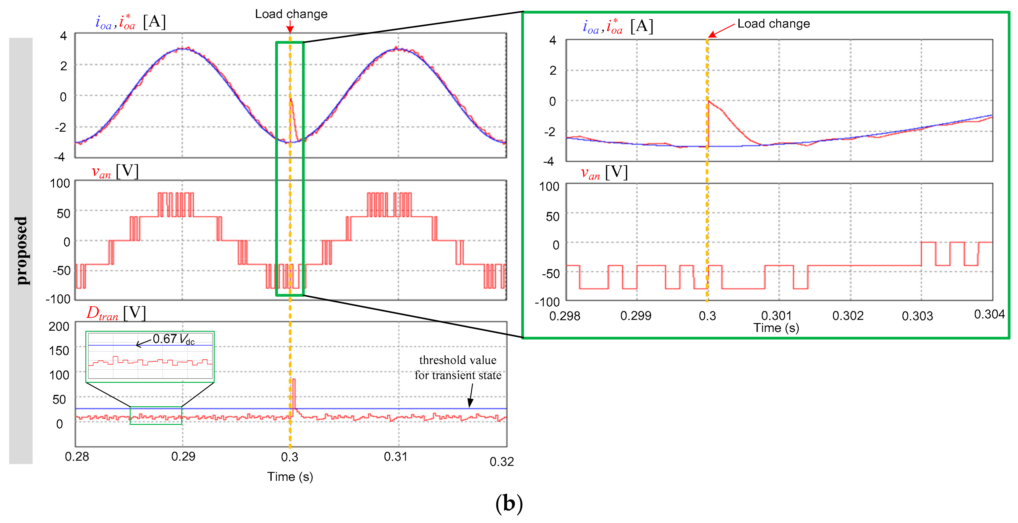
Contrary to the steady state, the proposed method defines a new candidate vector subset for the transient state, which consists of more vectors than those in the subset used for the steady state in order to overcome the slow transition speed of the MPC-conv2 method. This paper compares an optimal voltage vector at a present step with a reference voltage vector at a next step to identify the next step as a transient state. By using voltage vectors instead of current vectors, larger identification values can be achieved to interpret a next step as either a transient or a steady state. As shown in Figure 5, if the one-step future reference voltage vector calculated in Equation (15) is located inside the smallest hexagon centered at the present optimal voltage vector in the αβ plane, the developed algorithm interprets the next step as a steady-state condition. On the other hand, in a case where the reference voltage vector at the next step is positioned outside the hexagon, the algorithm describes, instead, a transient state, as shown in Figure 5. Therefore, the difference between two nearest voltage vectors in the αβ plane is used to identify a next step as a transient or a steady state. A determinant factor, Dtran, to indicate that the transient condition occurs at the next step is defined as:
where, and represent the α and β component of the optimal voltage values at a present step, respectively. In addition, a value of 0.67Vdc indicates the distance between the two closest voltage vectors in the αβ plane. It should be noted that, because the proposed determinant algorithm is based on voltage vectors determined in the αβ plane, the distinction between steady state and transient state is free from switching ripple components and noise, thus highlighting the robustness of the algorithm. In the case that the proposed algorithm recognizes a transient state based on the determinant factor, it uses a new candidate vector subset, which consists of more voltage vectors than those in the subset used for the steady state, to achieve a much faster process compared to the MPC-conv2 method, but almost the same fast dynamic response as the MPC-conv1 method using all the voltage vectors. Furthermore, in comparison with the MPC-conv1 method, the proposed method employs fewer vectors than all possible vectors generated by the multilevel CHB inverter for calculation simplicity. Thus, the proposed method can offer almost the same fast transient response as the MPC-conv1 method using all the possible vectors, but with reduced calculation complexity in transient states as well as in steady states.
The proposed method determines an optimal vector during transient states by utilizing a new subset, which results in an excellent transient response performance. Figure 6 shows the candidate voltage vectors considered using the proposed method during the transient states. The candidate voltage vectors in the proposed method are chosen in such a way that the difference between a reference voltage vector and its closest candidate vector is less than 0.67Vdc, no matter in which position a reference vector is located in the αβ plane. We selected the shapes of the vectors in Figure 6, by selecting all the voltage vectors in one row and rejecting all the vectors in the other row. This is because we wished to select the candidate vectors in such a way that an optimal vector selected by the proposed method would be as close as possible to an optimal vector selected by the MPC-conv1 method using all the vectors, to use a reduced set of voltage vectors without significantly deteriorating the dynamic speed. This subset of the candidate vectors for transient conditions can produce almost the same fast dynamic response as the MPC-conv1 method using all the voltage vectors. In the transient state, a cost function, htran, is used, which considers the new candidate voltage vectors shown in Figure 6, instead of the adjacent vectors of the present reference voltage vector in the MPC-conv2 method, or all the possible voltage vectors in the MPC-conv1 method. The total number of the candidate voltage vectors used for the transient state in the proposed method is nearly half of all the possible voltage vectors, as evident in Figure 6. The cost function for the transient state, htran, is defined as:
where, and represent the α and β components of the one-step future voltage vectors, respectively, as shown in Figure 6. As a result, the proposed method offers much faster dynamic responses than the MPC-conv2 method under the transient conditions. Furthermore, in comparison with the MPC-conv1 method, the proposed method under transient conditions produces almost the same transient speed and lower calculation complexity (reduced by nearly half).
Figure 7 shows how the proposed method and the MPC-conv1 method select optimal voltage vectors under transient conditions. Assume that both methods select V28 as the optimal vector at the kth step because it is the closest one to the reference vector at the present step . In the case that a reference vector, , moves at (k + 1)th step because of a transient state, as shown in Figure 7a, it is seen that both the proposed and the MPC-conv1 methods select the vector V18 as the optimal vector, which makes the two methods produce the same dynamic response. If a reference vector, , moves at (k + 1)th step, as shown in Figure 7b, the MPC-conv1 method, considering all the voltage vectors, chooses V50 as the optimal vector at (k + 1)th step, which is the nearest one to the reference voltage. On the other hand, the proposed method selects the vector V49 as the optimal vector at (k + 1)th step, because the reduced set of the proposed method does not include the voltage vector V50. Although the proposed method yields a slightly slower dynamic response than the MPC-conv1 method because of the reduce set of candidate voltage vectors, it should be noted that the two vectors, V49 and V50, selected by the proposed and the MPC-conv1 methods, respectively, are adjacent vectors with a difference of 0.67Vdc. Thus, the selection processes of the optimal voltage vectors by the two methods are similar after the transitions, and, therefore, the proposed method can reduce the computational complexity of the algorithm without significantly reducing the dynamic speed.
Figure 8 shows a flow chart of the proposed algorithm, which distinguishes between a steady and transient state for a next step by calculating the determinant factor Dtran.
4. Simulation and Experimental Results
The developed MPC method was tested via computer simulations using a five-level CHB inverter, which consists of two cells with separate DC power sources (Vdc = 40 V). A sampling period, Ts, of 200 μs and an R-L load of (R = 20 Ω and L = 15 mH) were used in the simulation. Simulations with the two conventional methods, the MPC-conv1 and MPC-conv2 methods, were carried out for comparison purpose with the proposed method. Figure 9 and Figure 10 show the three-phase load currents and the Fast Fourier Transform (FFT) analysis of the a-phase load current during steady states, obtained using the two conventional methods and the proposed method. The three methods show the same performance under steady-state conditions. Moreover, the total harmonic distortion (THD) values obtained by all three methods are the same, as shown in Figure 10. It can be seen that the proposed and the MPC-conv2 methods, both of which use only neighboring voltage vectors of a present optimal vector, produce the same quality in terms of load current waveforms and frequency spectrum as the MPC-conv1 method that utilizes all the possible voltage vectors. Because the sampling frequency is much faster than the frequency of the reference voltage, the trajectory of the optimal voltage vector changes very slightly during one sampling period in steady state. Therefore, considering only the adjacent voltage vectors of a present optimal vector is enough to determine a next-step optimal vector.
Figure 11 shows the simulated waveforms of the a-phase reference current, a-phase actual current, and a determinant value Dtran under a transient-state condition, such as a magnitude change of the reference currents from −3 A to 1.5 A, a frequency change of the reference currents from 50 Hz to 75 Hz, and a load change from 20 Ω to 10 Ω in the proposed method. During the step-changes in the reference current magnitude and the load resistance in Figure 11a,c, it can be observed that the determinant value Dtran is kept below the threshold value to interpret a next step as a steady state before the transient conditions occur. However, the value quickly increases in both plots under transient conditions. Once the transient phase has lapsed in both plots, the determinant value Dtran decreases to a value lower than the threshold value. On the other hand, it can be seen from Figure 10b that the value Dtran remains lower than the threshold value, irrespective of the step-change in frequency of the reference currents. This is because the frequency change produces only rotational speeds of the reference current and voltage vectors without changes in magnitude. Therefore, similar to the steady states, the step-change in the frequency of the reference currents can be quickly followed by considering only the adjacent vectors of an optimal voltage vector. The determinant value Dtran can then be utilized to accurately identify a transient state with recognizable values between steady states and transient states.
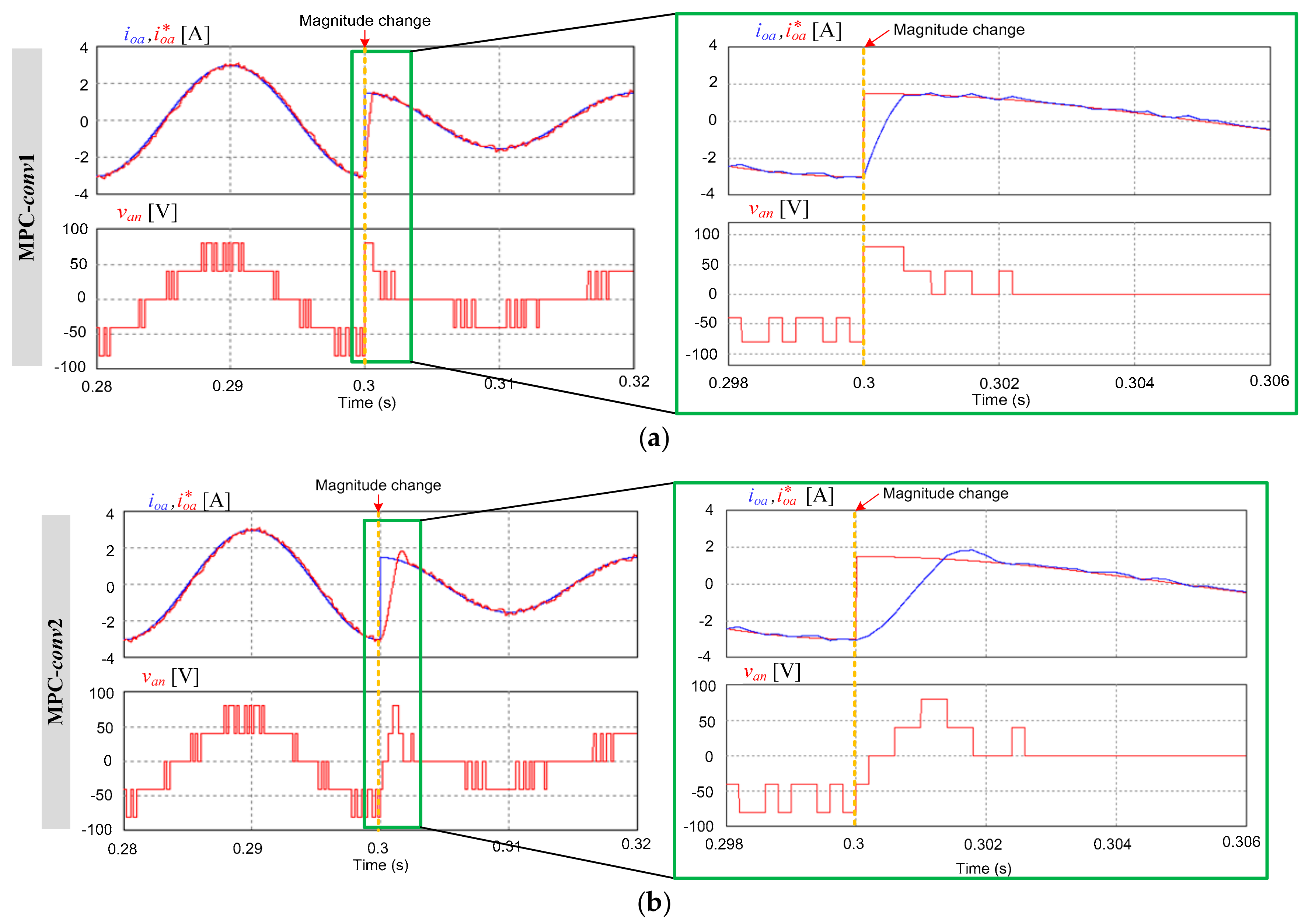
Figure 12 shows the simulation results of the a-phase load current (ioa), a-phase reference current (), and a-phase inverter voltage (van) obtained using the three methods during the transient state of a magnitude change of reference currents. Although all three methods demonstrate the same steady-state performance as shown in Figure 9 and Figure 10, they exhibit different transient responses with different inverter voltage waveforms, as shown in Figure 12. Obviously, the MPC-conv2 method, which considers only seven vectors inside the smallest hexagon near the present optimal vector for the sake of reduced computational load, produces a slow transient response when a transient state occurs. In contrast, the actual load current generated by the MPC-conv1 method at the expense of the high computational load associated with the consideration of all vectors, tracks its reference value faster than the MPC-conv2 method. It is evident from Figure 12 that the proposed method, which reduces the number of candidate vectors in comparison with the MPC-conv1 method, can force the actual load current to follow its reference value as fast as the MPC-conv1 method. In addition, it is shown that the inverter-phase voltage waveform obtained using the proposed method is the same as that of the MPC-conv1 method, despite a reduced number of candidate voltage vectors.
Figure 13 shows the simulation results of the a-phase load current (ioa), a-phase reference current (), and a-phase voltage (van) obtained using the three methods during the transient state of a frequency change in the reference currents. Unlike the magnitude step-change of the reference currents in Figure 12, all three methods produced the same results in the frequency step-change of the reference currents as shown in Figure 13. In Figure 11b, only the frequency change of the reference currents does not result in an abrupt increase of the current and voltage vectors before and after the step-change in the αβ plane. Thus, fast dynamics can be achieved by considering only the adjacent vectors of an optimal vector at a present step.
Figure 14 shows the simulation results of the a-phase load current (ioa), a-phase reference current (), and a-phase voltage (van) obtained using the three methods during the transient state of a load change. Like the magnitude step-change of the reference currents in Figure 12, different transient responses are exhibited in Figure 14. It is clearly seen in Figure 14 that the proposed and MPC-conv1 methods produced the same fast transient responses as well as the same inverter voltage waveforms, whereas the MPC-conv2 method, with only the neighboring voltage vectors, produces a slow transient response. Therefore, it can be inferred that the proposed method can achieve a fast dynamic speed, similar to the MPC-conv1 method, despite a reduced number, by approximately a half, of candidate voltage vectors.
The dynamic speeds of the actual load currents obtained from all three methods under transient conditions are compared in Figure 15, during step-change in the reference current magnitude from −3 A to −1.5 A, reference current frequency from 50 Hz to 75 Hz, and load change from 20 Ω to 10 Ω. In the case of the magnitude change of the reference current from −3 A to −1.5 A, as shown in Figure 15a, the MPC-conv2 method experiences the transient period for ~0.8 ms, which corresponds to four sampling periods. On the other hand, the transient period of the proposed method, which is almost the same as that of the MPC-conv1 method, is 0.2 ms, corresponding to one sampling period. Figure 15b shows the step-change of the reference current magnitude from −3 A to 1.5 A, which is a larger current change than in Figure 15a. The MPC-conv2 method undergoes the transient phase for 2.4 ms, whereas the proposed and the MPC-conv1 methods complete the transient period after approximately 0.6 ms. Therefore, the proposed method presents load current dynamics that is four times faster than that of the MPC-conv2 method in both cases. Furthermore, the proposed method exhibits a transient response as fast as the MPC-conv1 method, even when considering that it requires approximately half less voltage vectors than the MPC-conv1 method. In the case of the frequency change of the reference current from 50 Hz to 75 Hz, there is no observable difference in each method, as shown in Figure 15c. As depicted in Figure 15d, in the case of the load change, the transient response time of the MPC-conv2 takes 1.7 ms, while it takes 0.6 ms in the case of the proposed and the MPC-conv1 methods. As a result, the proposed method results in a dynamic speed that is as fast as that of the MPC-conv1 method in the step-changes, even with a reduced calculation complexity during the transient states. However, the reduced set of voltage vectors used in the proposed method can lead to a deteriorated performance, which corresponds to a slower dynamic speed, depending on the transition conditions. The proposed method can have exactly the same performance as the MPC-conv1 in transient or can show a slightly slower dynamic speed than the MPC-conv1, depending on the transient conditions. A variety of transient conditions were applied to thoroughly compare the responses of the proposed and the MPC-conv1 methods. Figure 16 and Figure 17 show the simulation results of the a-phase load current (ioa), a-phase reference current (), and a-phase inverter voltage (van) obtained using the MPC-conv1 and the proposed methods during the transient state of reference current changes from −3 A to −2.5 A and 3 A, respectively. It is seen that the proposed method, under these transient conditions, generates exactly the same waveforms of the load currents and the inverter-phase voltages as the MPC-conv1 method, despite a reduced number of candidate voltage vectors.
In addition, Figure 18 and Figure 19 show the simulation results of the a-phase load current (ioa), a-phase reference current (), and a-phase inverter voltage (van) obtained using the MPC-conv1 and the proposed methods during the transient state of load changes from 20 Ω to 19 Ω and 5 Ω, respectively. It is seen that the proposed method, under these transient conditions, generates exactly the same waveforms of the load currents and the inverter phase voltages as the MPC-conv1 method, despite a reduced number of candidate voltage vectors.
Figure 20 and Figure 21 illustrate the simulation results of the a -phase load current (ioa), a-phase reference current (), and a-phase inverter voltage (van), and the numbers of the optimal voltage vectors obtained using the MPC-conv1 and the proposed methods during the transient state of changes in the phase angles as well as in the magnitudes of the reference currents. Under these transient conditions, it is shown that the proposed method yields different inverter-phase voltage waveforms compared to the MPC-conv1 method during a couple of the sampling periods after the transition instants, because of the different selection of the optimal voltage vectors derived from the reduced set of candidate voltage vectors. However, it is clearly seen that the inverter-phase voltage waveforms as well as the selected optimal voltage vectors obtained by the two methods become exactly the same a couple of the sampling periods after the transition instants. In addition, the dynamic speeds of the load current waveforms of the proposed methods are almost the same as those of the MPC-conv1 method. Thus, the deterioration of the transient dynamics of the proposed method at the expense of the reduced set of voltage vectors is negligible, as shown in Figure 20 and Figure 21, although the proposed method might lead to a very slightly slower dynamic speed than the MPC-conv1 method under some transient conditions.
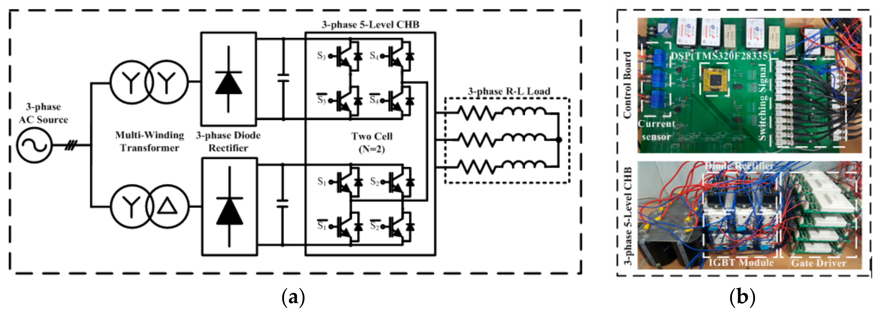
To verify the proposed method, a prototype of the three-phase five-level CHB inverter was fabricated with single-phase full bridge inverter modules (Infineon F4-30R06W1E3). The two conventional MPC methods (MPC-conv1 and MPC-conv2 methods) and the proposed method were implemented using digital signal processor (DSP) boards (TMS320F28335). The experiments were carried out to create sinusoidal load currents with a fundamental frequency of 60 Hz using the same sampling period (Tsp = 200 μs) and R-L load (R = 20 Ω, L = 15 mH) as in the simulation tests. Each module was supplied with a separate DC voltage (Vdc = 40 V) using diode rectifiers connected to a multiwinding transformer. A block diagram and a prototype photograph of the five-level CHB inverter are shown in Figure 22.
Figure 23 shows the experimental results of the three-phase load current, a-phase reference current, a-phase inverter-phase voltage, and ab line–line voltage under the steady-state condition. Similar to the simulation results, the three methods produce the same sinusoidal current and voltage waveforms with high quality and the a-phase load current tracking its reference current in the steady state.
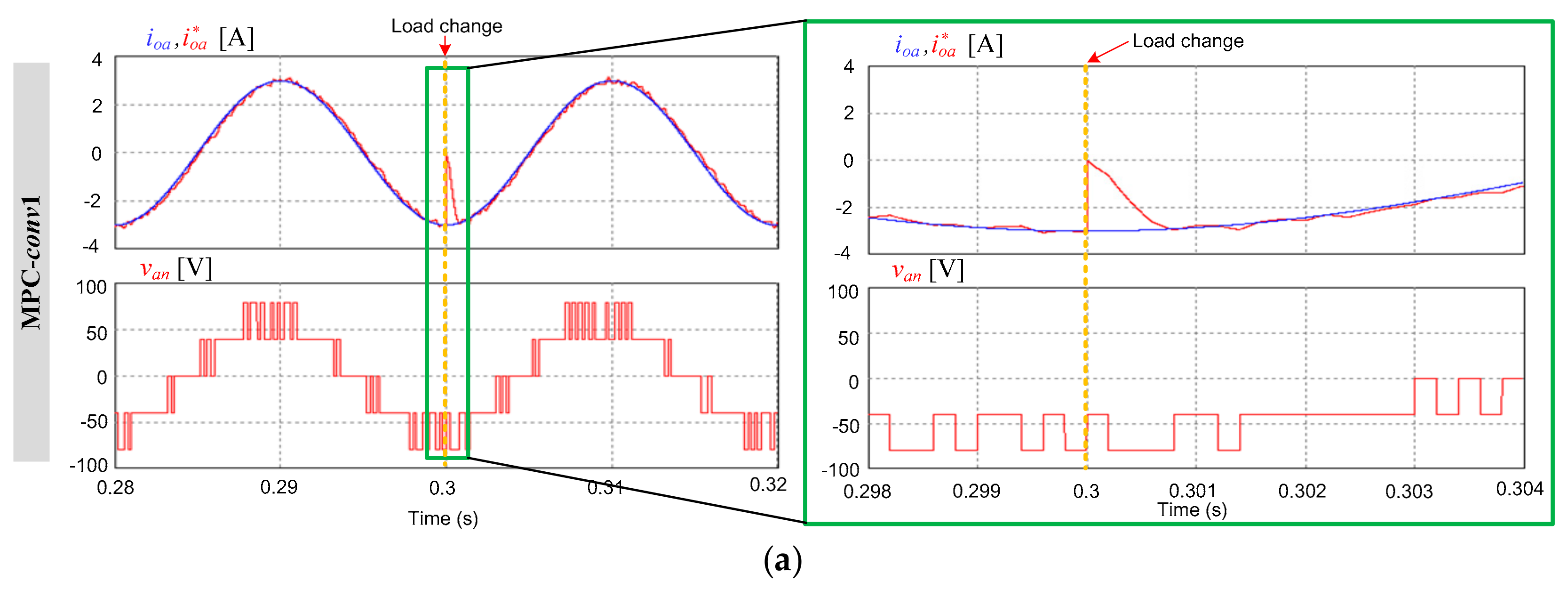
Figure 24 shows the experimental waveforms of the a-phase load current, a-phase reference current, and a-phase inverter output voltage obtained using the three methods, during a transient state where the magnitude of the reference current is suddenly changed from −3 A to 1.5 A. The actual currents from both the conventional and proposed methods accurately follow their reference current, however, with different dynamic speeds depending on each algorithm. It is obvious from Figure 24 that the proposed method has the same dynamic speed as the MPC-conv1 method, which is faster that the MPC-conv2 method. The magnified experimental waveforms during the transient periods are also shown in Figure 24, to clearly illustrate the dynamic performance of the three methods. It can be seen that the proposed method results in load current dynamics that is as fast as the MPC-conv1 method and even much faster than the MPC-conv2 method. In addition, it is shown that the inverter-phase voltage waveform obtained using the proposed method is the same as that of the MPC-conv1 method, although the proposed method utilizes approximately half less candidate voltage vectors compared to the MPC-conv1 method.
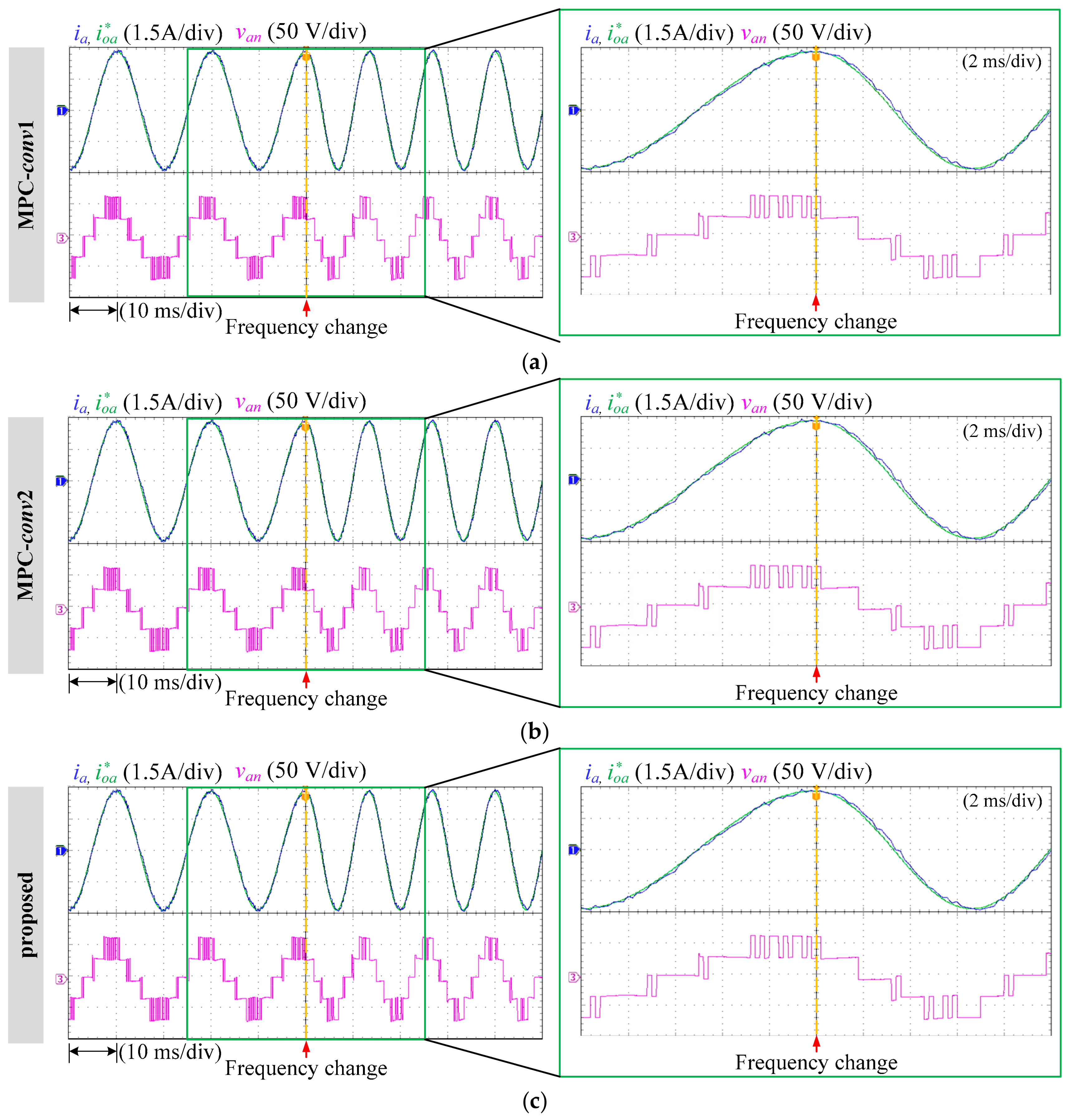
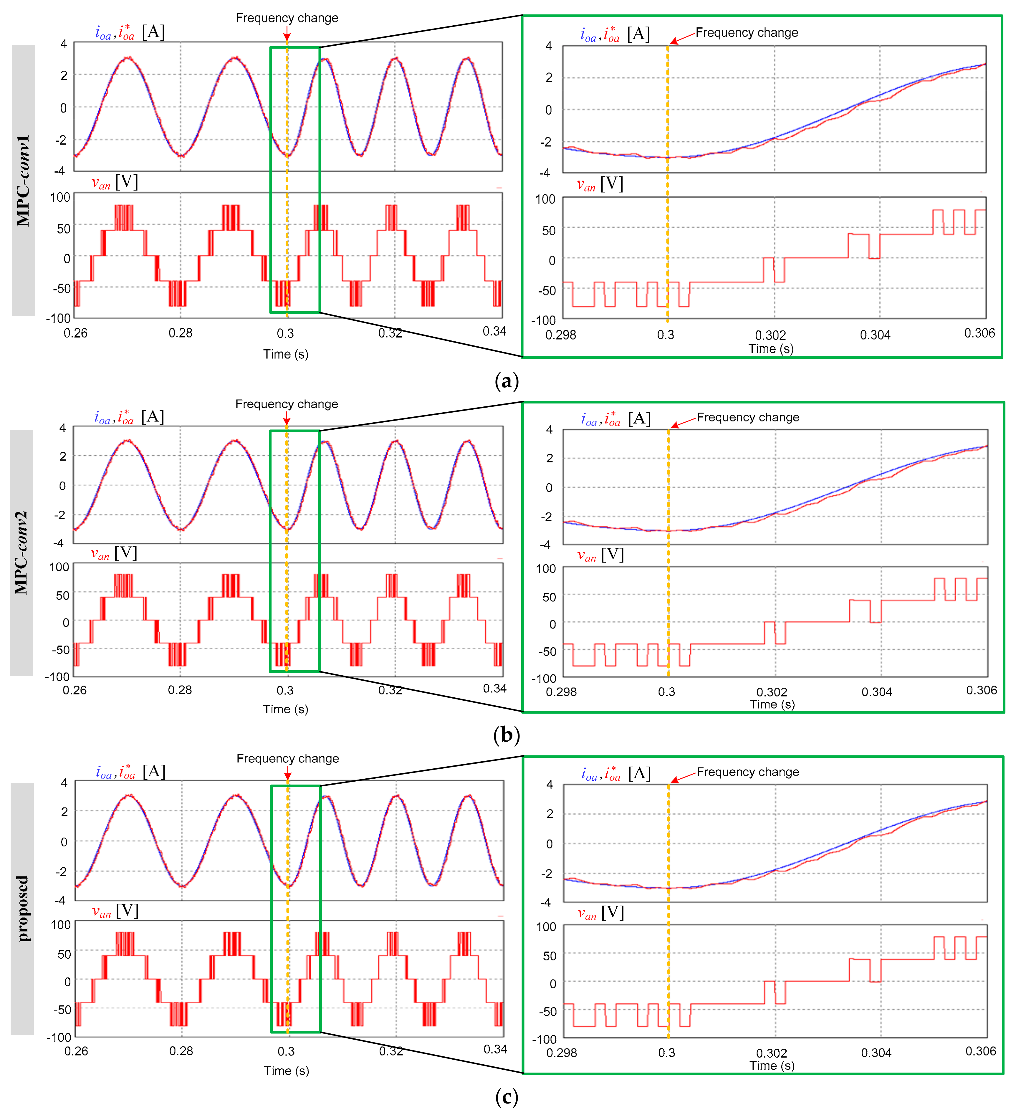
Figure 25 shows the experimental results of the a-phase load current, the a-phase reference current, the a-phase voltage obtained with the three methods during the transient state of a frequency change in the reference currents. As for the simulation results with the frequency step-change in Figure 13, the three methods yield the same experimental results because of the smooth rotation of the current and voltage vector with no sudden movement before and after the step-change in the αβ plane.
In the experimental setup, the number of clocks in the digital signal processor (DSP) board was measured for calculating the time required to perform the entire algorithm of the conventional (MPC-conv1 and MPC-conv2) and proposed methods. The DSP execution time calculated by the number of DSP clocks, THD values, and current errors are summarized in Table 2 to compare the experimental results obtained using the three methods. In comparison with the MPC-conv1 method, the proposed method requires an execution time of approximately 25% and 50% in steady and transient states, respectively. The current quality performances, such as the THD values and the current errors, are the same for all three methods. The dynamic response speed of the proposed MPC method is almost the same as that of the MPC-conv1 method, but much faster than that of the MPC-conv2 method.
5. Conclusions
This paper has presented an MPC algorithm with reduced computational complexity and fast dynamic response for multilevel CHB inverters, in which different candidate vector subsets to determine an optimal voltage vector are respectively developed for steady and transient states. The proposed method presents a robust technique for interpreting a next step as either a steady or transient state by comparing an optimal voltage vector at a present step and a reference voltage vector at the next step. Because the proposed determinant algorithm is based on voltage vectors determined in the αβ plane, the distinction between steady state and transient state is free from switching ripple components and noise. During steady state, only seven voltage vectors inside the smallest hexagon near a present optimal voltage vector are considered as a candidate-vector subset. On the other hand, a new candidate vector subset for the transient state is defined, which consists of more vectors than those in the subset used for the steady state for fast dynamic speed; however, the vectors are less than all the possible vectors generated by the CHB inverter for calculation simplicity. The proposed method determines an optimal vector during the transient state by utilizing the new subset, which results in an excellent transient response performance. As a result, the proposed method, compared to the conventional methods, can reduce the computational complexity without significantly deteriorating the transient response.
Acknowledgments
This research was supported by the National Research Foundation of Korea (NRF) grant funded by the Korea government (MSIP) (2017R1A2B4011444) and the Human Resources Development (No.20174030201810) of the Korea Institute of Energy Technology Evaluation and Planning (KETEP) grant funded by the Korea government Ministry of Trade, Industry and Energy.
Author Contributions
All authors contributed to this work by collaboration.
Conflicts of Interest
The authors declare no conflict of interest.
References
- Ying, J.; Gan, H. High power conversion technologies and trend. In Proceedings of the 7th International Power Electronics and Motion Control Conference, Harbin, China, 2–5 June 2012; pp. 1766–1770. [Google Scholar]
- Marzoughi, A.; Burgos, R.; Boroyevich, D.; Xue, Y. Investigation and comparison of cascaded H-bridge and modular multilevel converter topologies for medium-voltage drive application. In Proceedings of the 40th Annual Conference of the IEEE Industrial Electronics Society, Dallas, TX, USA, 29 October–1 November 2014; pp. 1562–1568. [Google Scholar]
- Lai, J.S.; Peng, F.Z. Multilevel converters—A new breed of power converters. IEEE Trans. Ind. Appl. 1996, 32, 509–517. [Google Scholar]
- Carrasco, J.M.; Franquelo, L.G.; Bialasiewicz, J.T.; Guisado, R.C.P.; Parts, M.A.M.; Leon, J.I.; Moreno-Alfonso, N. Power Electronic Systems for the Grid Integration of Renewable Energy Sources: A survey. IEEE Trans. Ind. Electron. 2006, 53, 1002–1016. [Google Scholar] [CrossRef]
- Rodriguez, J.; Bernet, S.; Bin, W.; Pontt, J.O.; Kouro, S. Multilevel Voltage-Source-Converter Topologies for Industrial Medium-Voltage Drives. IEEE Trans. Ind. Electron. 2006, 53, 2930–2945. [Google Scholar] [CrossRef]
- Kouro, S.; Malionowski, M.; Gopakumar, K.; Pou, J.; Franquelo, L.G.; Bin, W.; Rodriguez, J.; Perez, M.A.; Leon, J.I. Recent Advances and Industrial Applications of Multilevel Converters. IEEE Trans. Ind. Electron. 2010, 57, 2553–2580. [Google Scholar] [CrossRef]
- Nabae, A.; Takahashi, I.; Akagi, H. A new neutral-point clamped PWM inverter. IEEE Trans. Ind. Appl. 1981, IA-17, 518–523. [Google Scholar] [CrossRef]
- Hammond, P. A new approach to enhance power quality for medium voltage ac drives. IEEE Trans. Ind. Appl. 1997, 33, 202–208. [Google Scholar] [CrossRef]
- Meynard, T.A.; Foch, H.; Thomas, P.; Courault, J.; Jakob, R.; Nahrstaedt, M. Multicell converter: Basic concepts and industry applications. IEEE Trans. Ind. Electron. 2002, 49, 955–964. [Google Scholar] [CrossRef]
- Qashqai, P.; Sheikholeslami, A.; Vahedi, H.; Al-Haddad, K. A Review on Multilevel Converter Topologies for Electric Transportation Applications. In Proceedings of the Vehicle Power and Propulsion Conference, Montreal, QC, Canada, 19–22 October 2015; pp. 1–6. [Google Scholar]
- Yu, Y.; Konstantinou, G.; Hredzak, B.; Agelidis, V.G. Power Balance of Cascaded H-Bridge Multilevel Converters for Large-Scale Photovoltaic Integration. IEEE Trans. Ind. Electron. 2016, 31, 292–303. [Google Scholar] [CrossRef]
- Rodriguez, J.; Lai, J.S.; Peng, F.Z. Multilevel inverters: A survey of topologies, controls, and applications. IEEE Trans. Ind. Electron. 2002, 49, 724–738. [Google Scholar] [CrossRef]
- Farivar, G.; Hredzak, B.; Agelidis, V.G. A DC-Side sensorless Cascaded H-Bridge Multilevel Converter-Based Photovoltaic System. IEEE Trans. Ind. Electron. 2016, 63, 4233–4241. [Google Scholar] [CrossRef]
- Mwinyiwiwa, B.N.; Wolanski, Z.; Ooi, B.T. Microprocessor implemented SPWM for multiconverters with phase-shifted triangle carriers. In Proceedings of the IEEE Industry Applications Conference Thirty-Second IAS Annual Meeting, New Orleans, LA, USA, 5–9 October 1997; pp. 1542–1549. [Google Scholar]
- Kouro, S.; Cortes, P.; Vargas, R.; Ammann, U.; Rodriguez, J. Model predictive control-A simple and powerful method to control power converters. IEEE Trans. Ind. Electron. 2009, 56, 1826–1838. [Google Scholar] [CrossRef]
- Kouro, S.; Perez, M.A.; Rodriguez, J.; Llor, A.M.; Young, H.A. Model predictive control: MPC’s role in the evolution of power electronics. IEEE Ind. Electron. Mag. 2015, 9, 8–21. [Google Scholar] [CrossRef]
- Vazquez, S.; Leon, J.; Franquelo, L.G.; Rodriguez, J.; Young, H.; Marquez, A.; Zanchetta, P. Model predictive control: A review of its applications in power electronics. IEEE Ind. Electron. Mag. 2014, 8, 16–31. [Google Scholar] [CrossRef] [Green Version]
- Kwak, S.; Park, J. Switching Strategy based on Model Predictive Control of VSI to Obtain High Efficiency and balanced Loss Distribution. IEEE Trans. Power Electron. 2014, 29, 4551–4567. [Google Scholar] [CrossRef]
- Vazquez, S.; Marquez, A.; Aguilera, R.; Quevedo, D.; Leon, J.I.; Franquelo, L.G. Predictive optimal switching sequence direct power control for grid-connected power converters. IEEE Trans. Ind. Electron. 2015, 62, 2010–2020. [Google Scholar] [CrossRef]
- Zhang, Y.; Wu, X.; Yuan, X.; Wang, Y.; Dai, P. Fast Model Predictive Control for Multilevel Cascaded H-Bridge STATCOM with Polynomial Computation Time. IEEE Trans. Ind. Electron. 2016, 63, 5231–5243. [Google Scholar] [CrossRef]
- Zhang, Y.; Wu, X.; Yuan, X. A Simplified Branch and Bound Approach for Model PredictiveControl of Multilevel Cascaded H-Bridge STATCOM. IEEE Trans. Ind. Electron. 2017, 64, 7634–7644. [Google Scholar] [CrossRef]
- Cortes, P.; Wilson, A.; Kouro, S.; Rodrguez, J.; Abu-Rub, H. Model Predictive Control of Multilevel Cascaded H-Bridge Inverters. IEEE Trans. Ind. Electron. 2010, 57, 3736–3743. [Google Scholar] [CrossRef]
- Jaroslaw, G.; Haitham, A.R. Speed Sensorless Induction Motor Drive with Predictive Current Controller. IEEE Trans. Ind. Electron. 2013, 60, 699–709. [Google Scholar]
- Cortes, P.; Rodriguez, J.; Silva, C.; Flores, A. Delay compensation in model predictive current control of a three-phase inverter. IEEE Trans. Ind. Electron. 2012, 59, 1323–1325. [Google Scholar] [CrossRef]
Figure 1.
(a) Three-phase multilevel Cascaded H-bridge (CHB) inverter with N cells; (b) structure of a cell.
Figure 1.
(a) Three-phase multilevel Cascaded H-bridge (CHB) inverter with N cells; (b) structure of a cell.

Figure 2.
Voltage diagram of the M-level CHB inverter with the number of redundant voltage vectors in the αβ plane.
Figure 2.
Voltage diagram of the M-level CHB inverter with the number of redundant voltage vectors in the αβ plane.
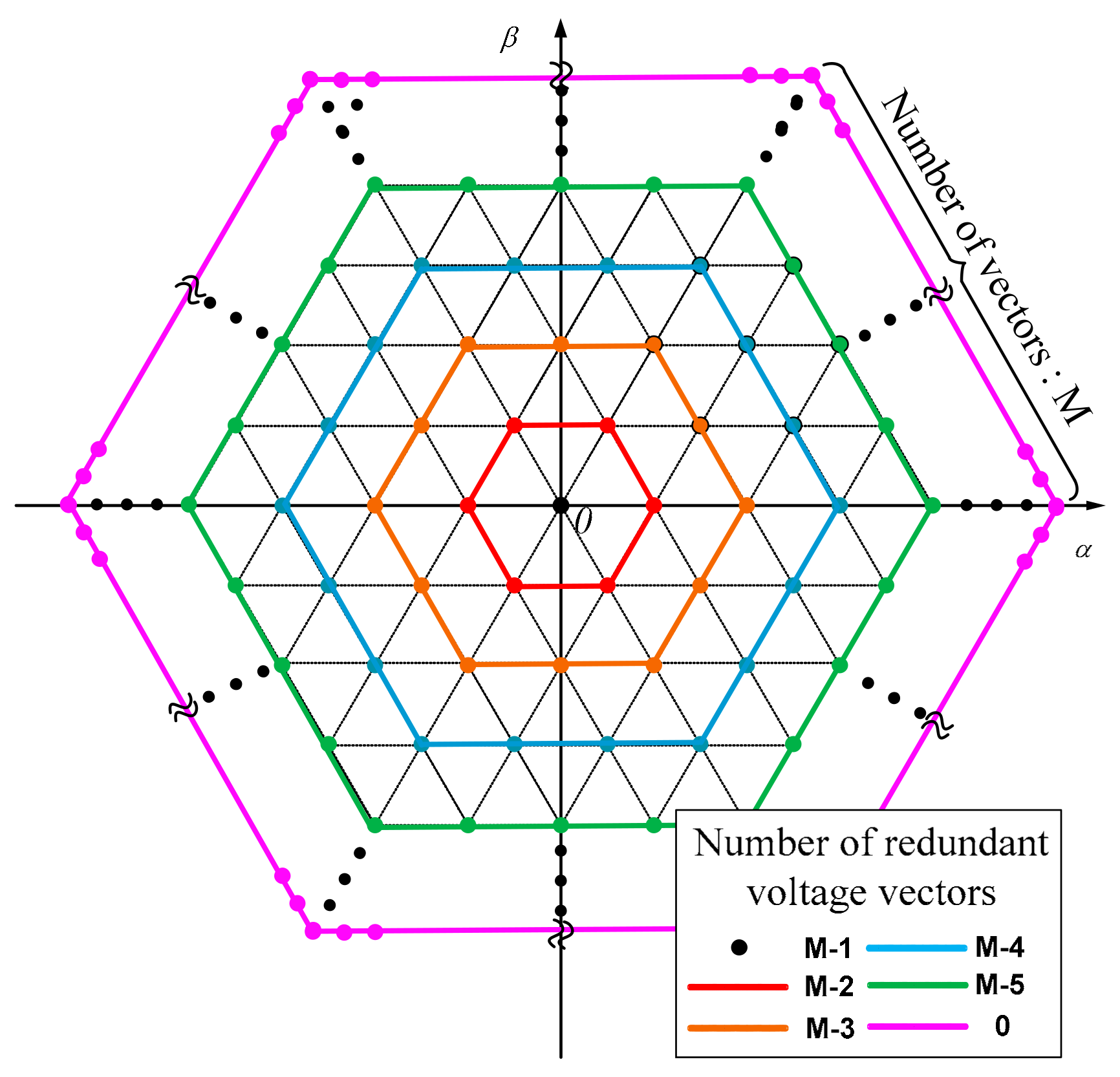
Figure 3.
Candidate voltage vectors in the model predictive control (MPC)-conv2 method in the case that a present optimal vector is V21.
Figure 3.
Candidate voltage vectors in the model predictive control (MPC)-conv2 method in the case that a present optimal vector is V21.

Figure 4.
Block diagram of the proposed finite-control-set model predictive control (FCS-MPC) method for a multilevel CHB inverter.
Figure 4.
Block diagram of the proposed finite-control-set model predictive control (FCS-MPC) method for a multilevel CHB inverter.

Figure 5.
Positions of a reference voltage vector at a next step and of an optimal voltage vector at a present step in the case of steady transient states in the proposed method.
Figure 5.
Positions of a reference voltage vector at a next step and of an optimal voltage vector at a present step in the case of steady transient states in the proposed method.
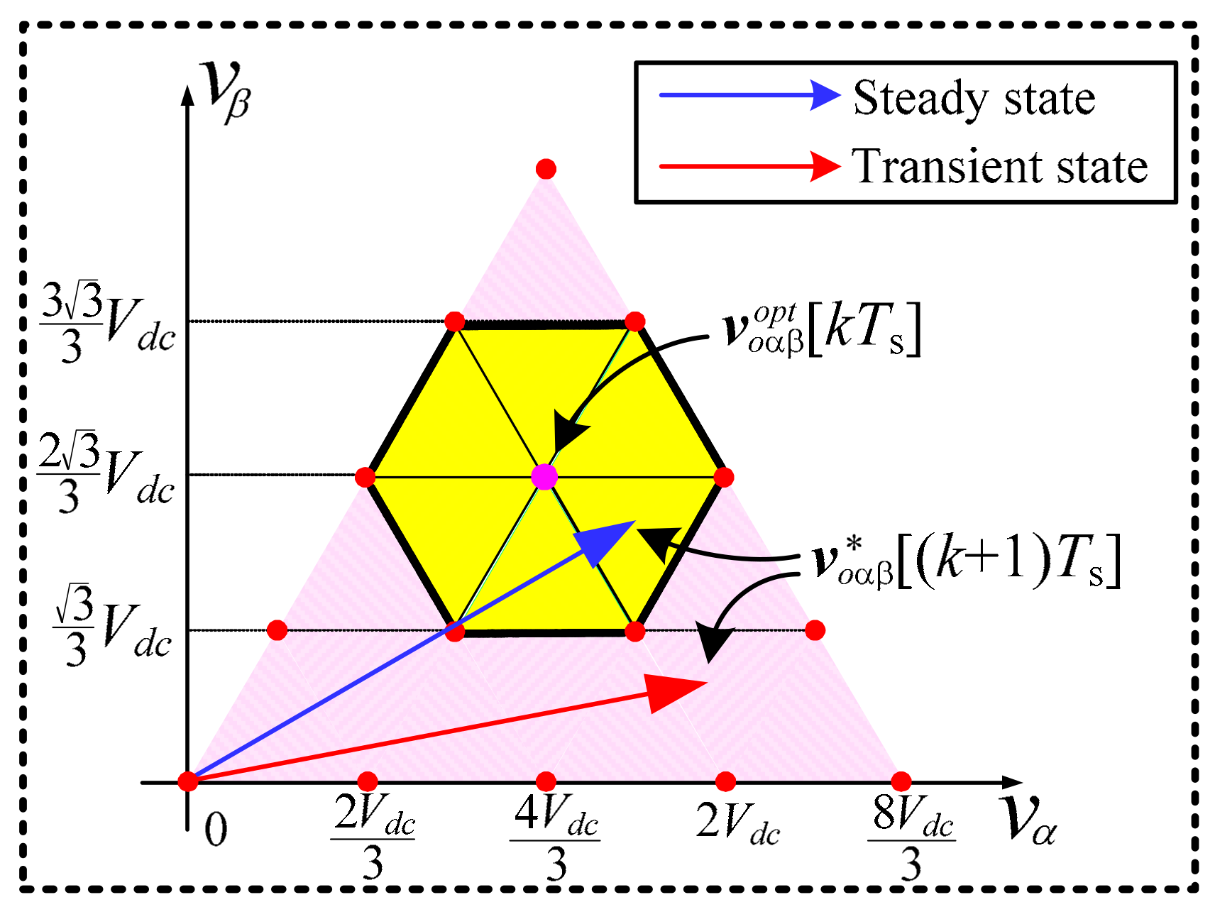
Figure 6.
Candidate voltage vectors considered during transient states using the proposed method for five-level CHB inverters.
Figure 6.
Candidate voltage vectors considered during transient states using the proposed method for five-level CHB inverters.
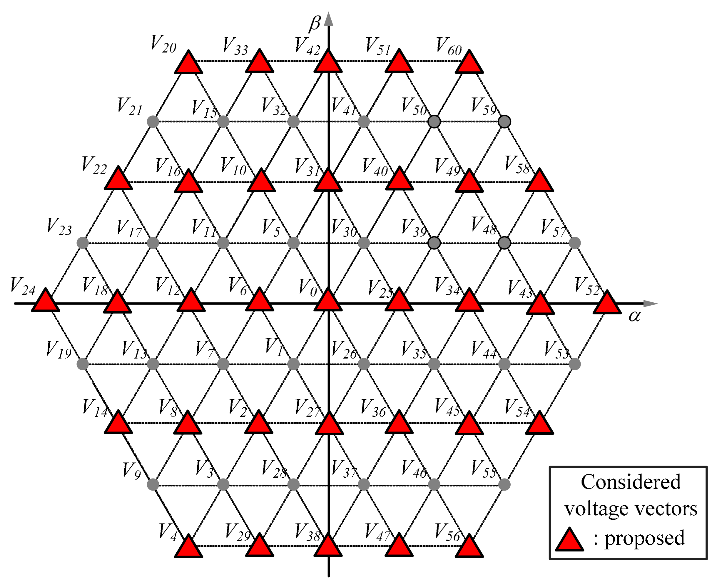
Figure 7.
Reference voltage vectors and optimal voltage vectors of the proposed and the MPC-conv1 methods under transient states (a) in the case that the proposed method and the MPC-conv1 method select the same optimal vectors (b) in the case that the proposed method and the MPC-conv1 method select different optimal vectors.
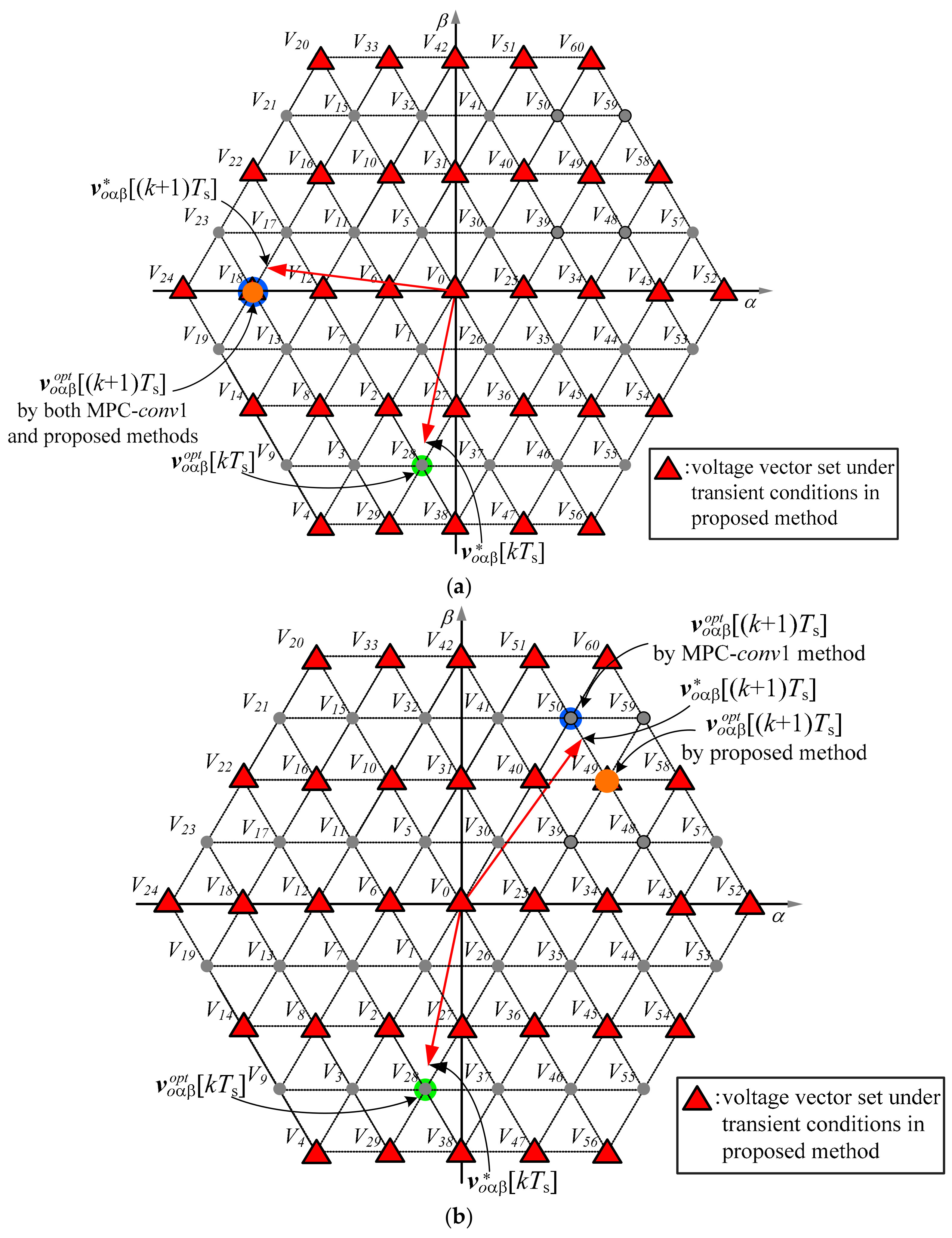
Figure 8.
Flow chart of the proposed method.
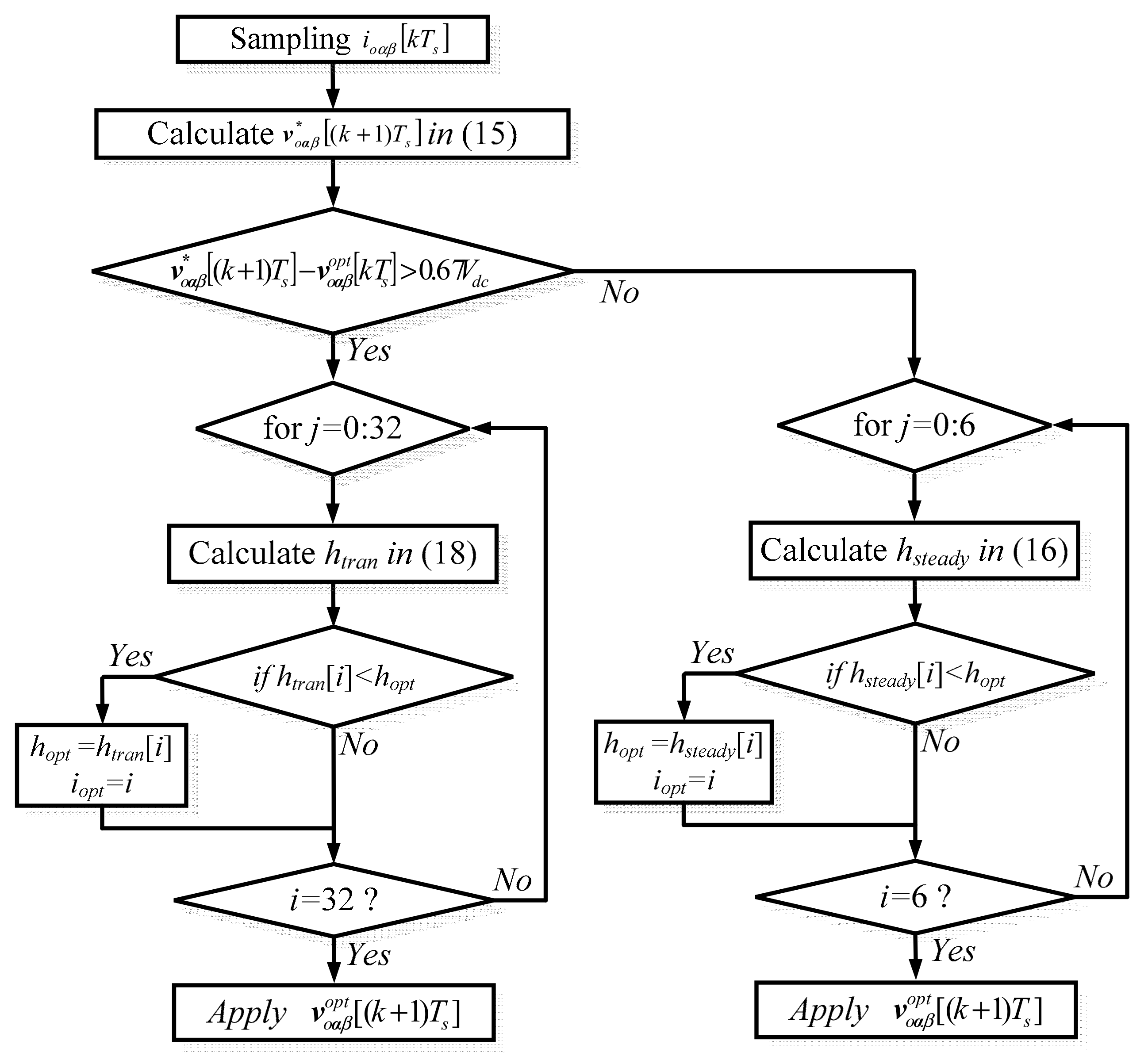
Figure 9.
Simulation waveforms of the three-phase load currents (ioa, iob, ioc) and the reference output current () in steady state from the (a) MPC-conv1 method, (b) MPC-conv2 method, (c) proposed method.
Figure 9.
Simulation waveforms of the three-phase load currents (ioa, iob, ioc) and the reference output current () in steady state from the (a) MPC-conv1 method, (b) MPC-conv2 method, (c) proposed method.
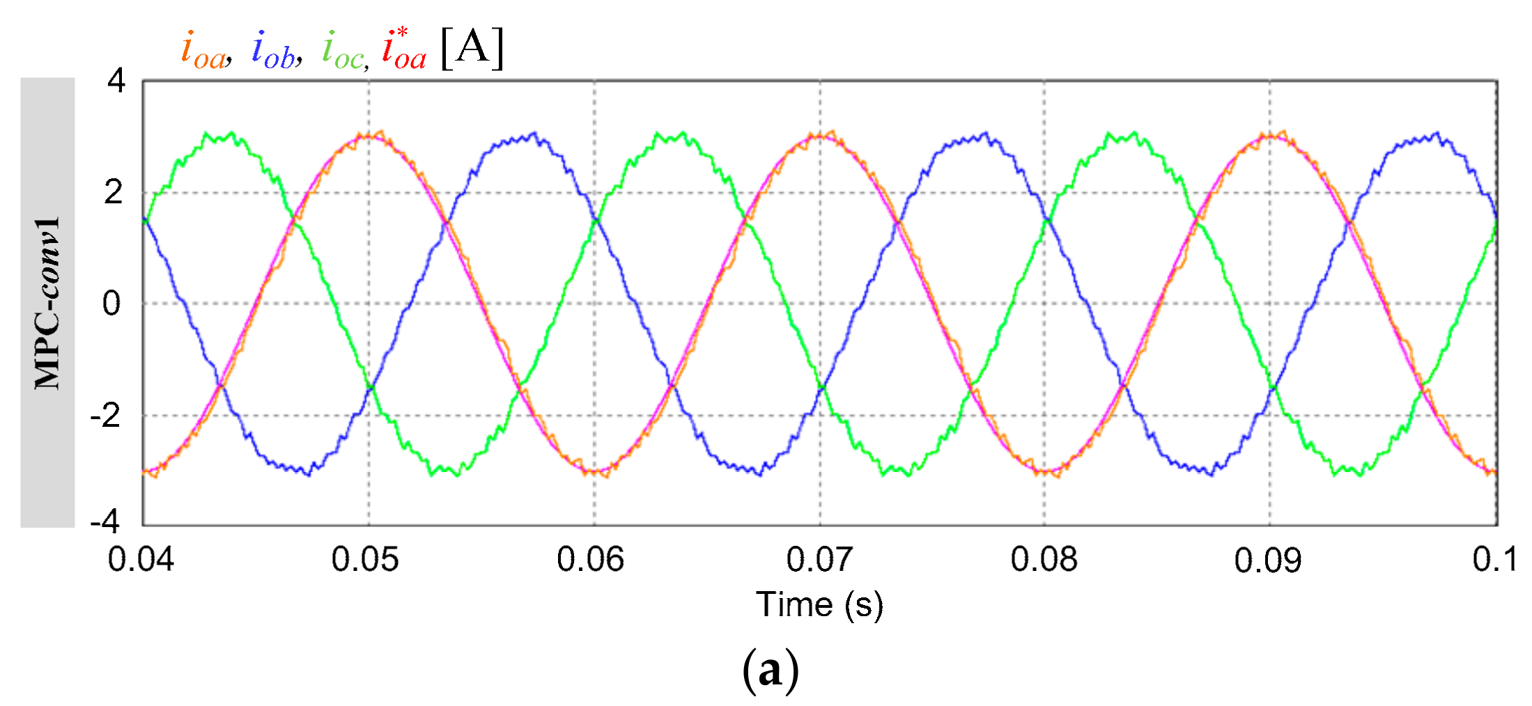
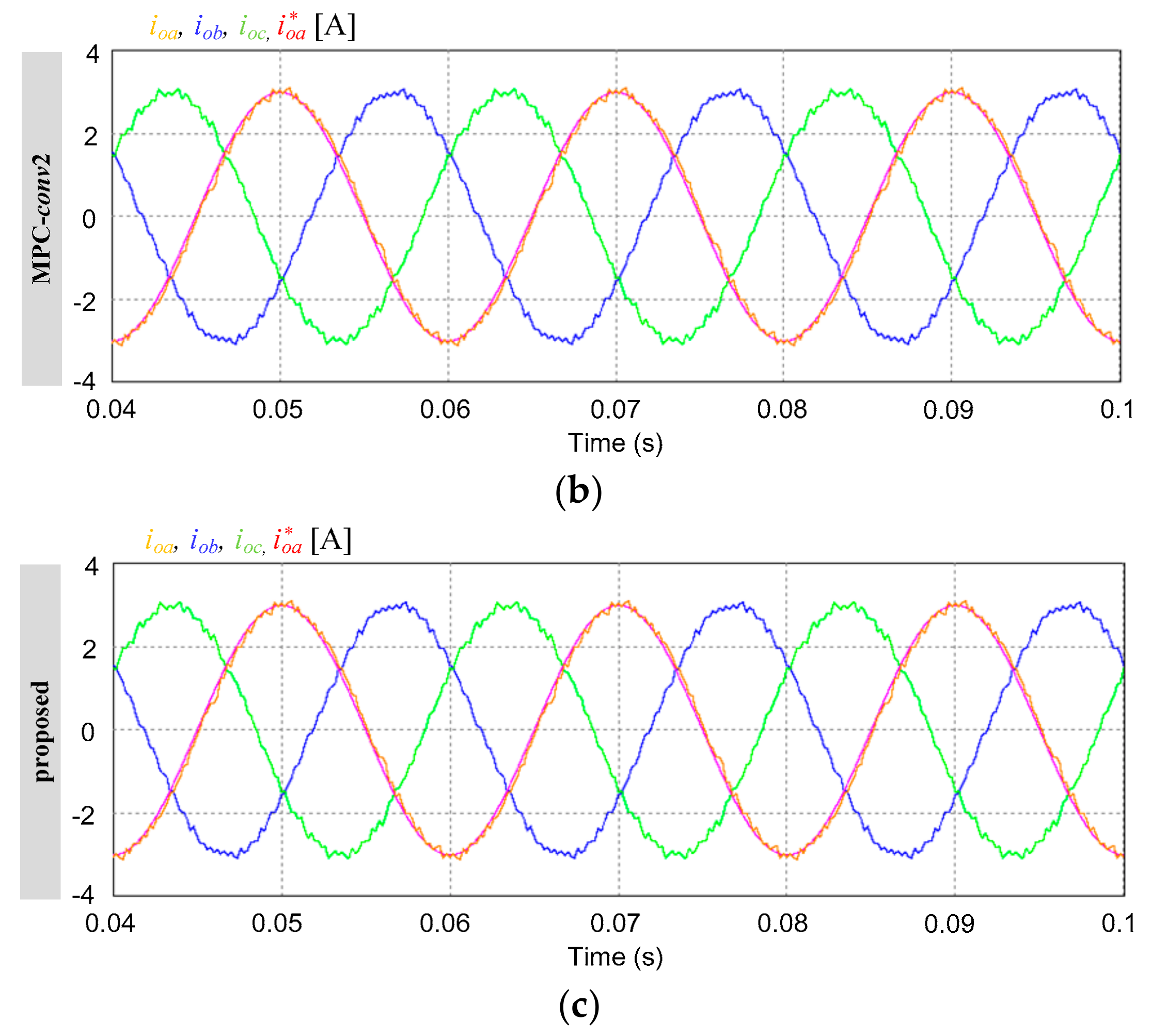
Figure 10.
Simulation waveforms of the Fast Fourier Transform (FFT) analysis of a-phase load currents (ioa) in steady state from the (a) MPC-conv1 method, (b) MPC-conv2 method, (c) proposed method.
Figure 10.
Simulation waveforms of the Fast Fourier Transform (FFT) analysis of a-phase load currents (ioa) in steady state from the (a) MPC-conv1 method, (b) MPC-conv2 method, (c) proposed method.
Figure 11.
Waveforms of the a-phase reference current, a-phase actual current, and a determinant value in the proposed method under transient-state condition. (a) Magnitude change of the reference currents from −3 A to 1.5 A, (b) frequency change of the reference currents from 50 Hz to 75 Hz, (c) load change from 20 Ω to 10 Ω.
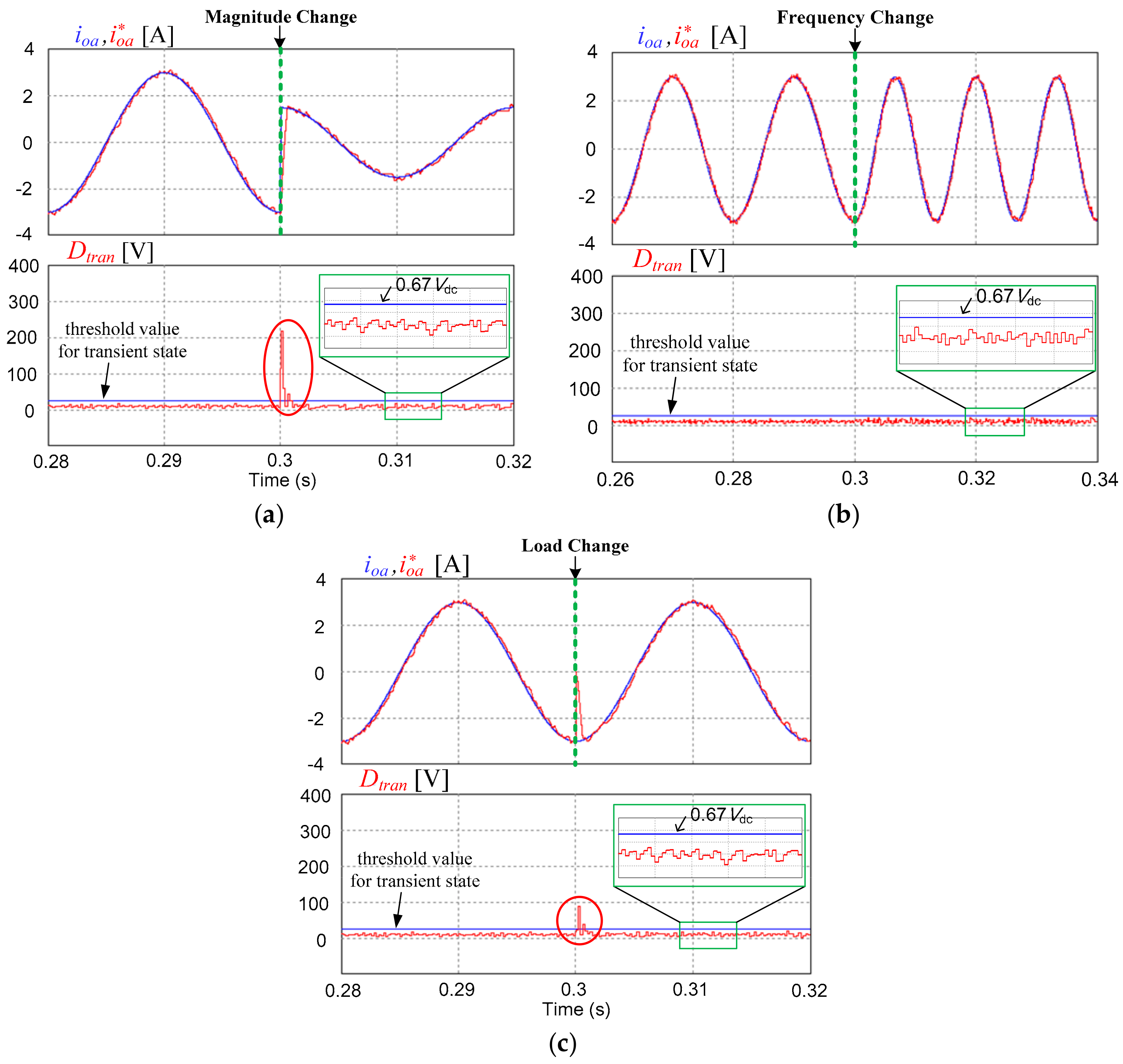
Figure 12.
Simulation waveforms of the a-phase actual current (ioa), a-phase reference current (), and a-phase inverter-phase voltage (van) during the transient state of the magnitude change of the reference currents from −3 A to 1.5 A obtained using the (a) MPC-conv1 method, (b) MPC-conv2 method, (c) proposed method.

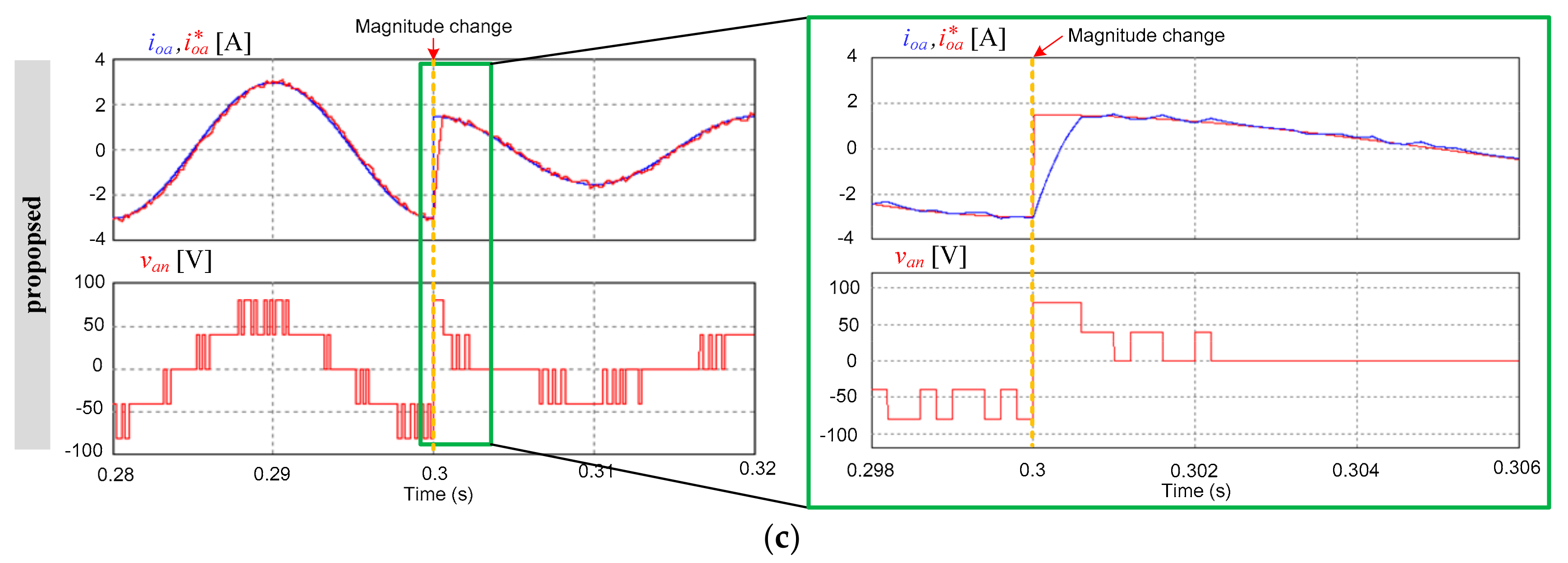
Figure 13.
Simulation waveforms of the a-phase actual current (ioa), a-phase reference current (), and a-phase inverter-phase voltage (van) during the transient state of a frequency change of the reference currents from 50 Hz to 75 Hz obtained using the (a) MPC-conv1 method, (b) MPC-conv2 method, and (c) proposed method.

Figure 14.
Simulation waveforms of the a-phase actual current (ioa), a-phase reference current (), and a-phase inverter-phase voltage (van) during the transient state of the load change from 20 Ω to 10 Ω obtained using the (a) MPC-conv1 method, (b) MPC-conv2 method, (c) proposed method.
Figure 14.
Simulation waveforms of the a-phase actual current (ioa), a-phase reference current (), and a-phase inverter-phase voltage (van) during the transient state of the load change from 20 Ω to 10 Ω obtained using the (a) MPC-conv1 method, (b) MPC-conv2 method, (c) proposed method.
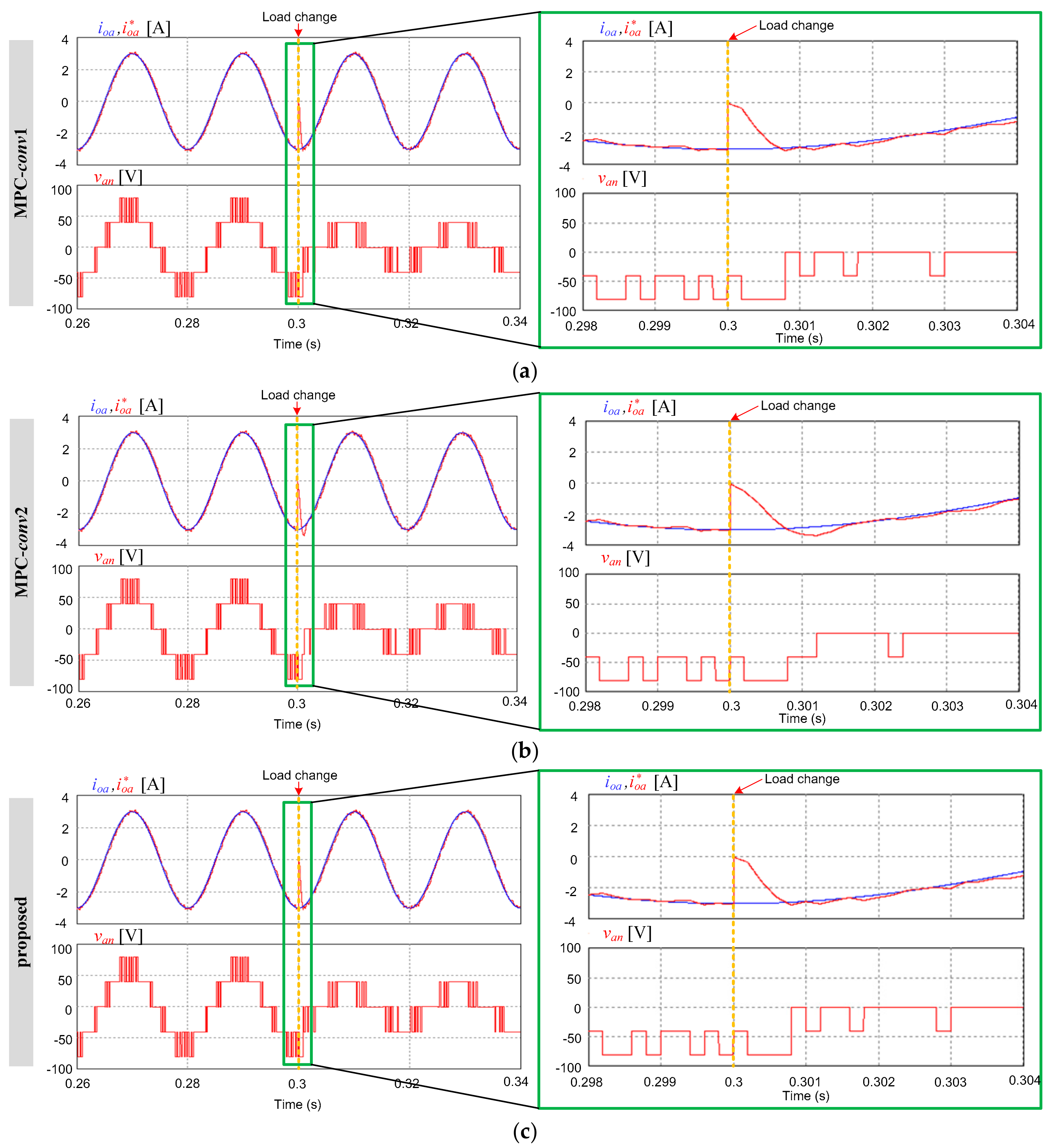
Figure 15.
Comparison of the dynamic speed of the actual load current waveforms obtained using the MPC-conv1, MPC-conv2, and proposed methods during step-change in (a) reference current magnitude from −3 A to −1.5 A, (b) reference current magnitude from −3 A to 1.5 A, (c) reference current frequency from 50 Hz to 75 Hz, (d) load change from 20 Ω to 10 Ω.
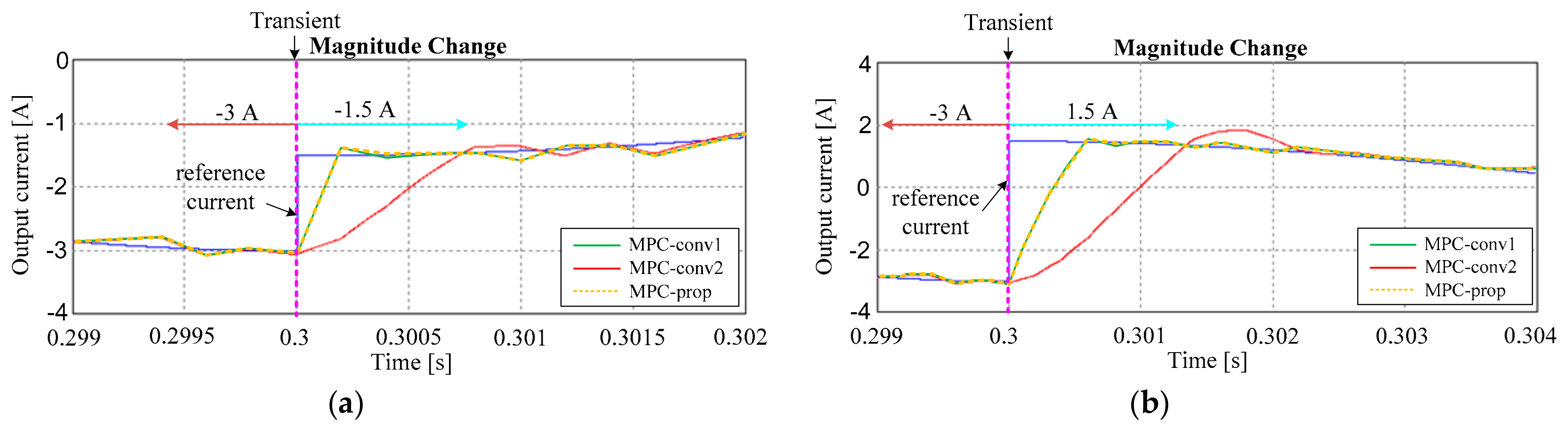
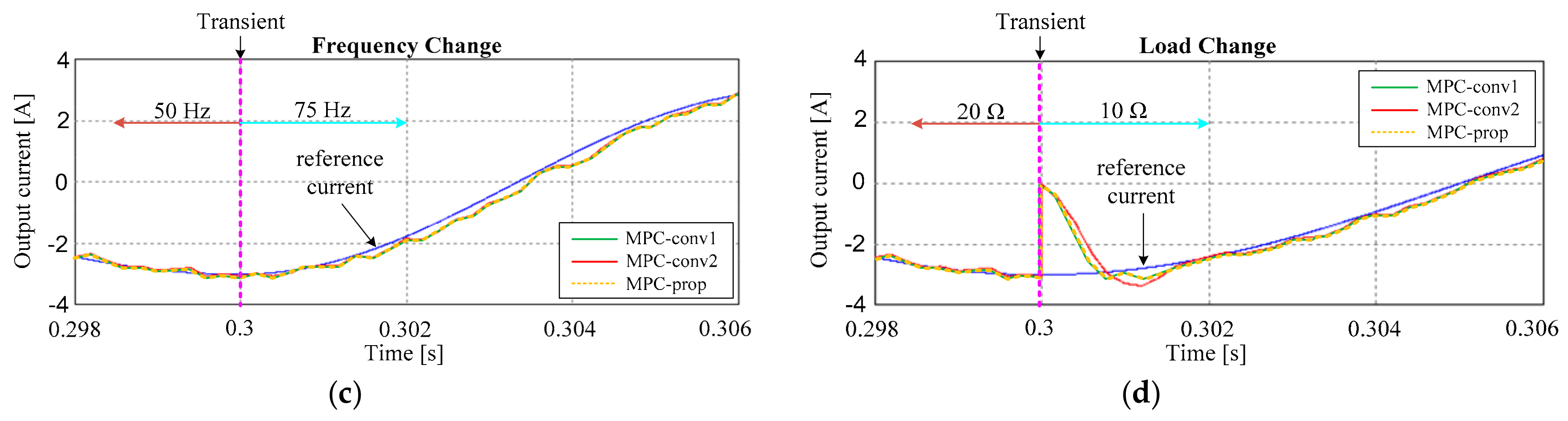
Figure 16.
Simulation waveforms of the a-phase actual current, a-phase reference current, and a-phase inverter phase voltage during the transient state of the reference current change from −3 A to −2.5 A obtained using (a) the MPC-conv1 method, (b) the proposed method.
Figure 16.
Simulation waveforms of the a-phase actual current, a-phase reference current, and a-phase inverter phase voltage during the transient state of the reference current change from −3 A to −2.5 A obtained using (a) the MPC-conv1 method, (b) the proposed method.
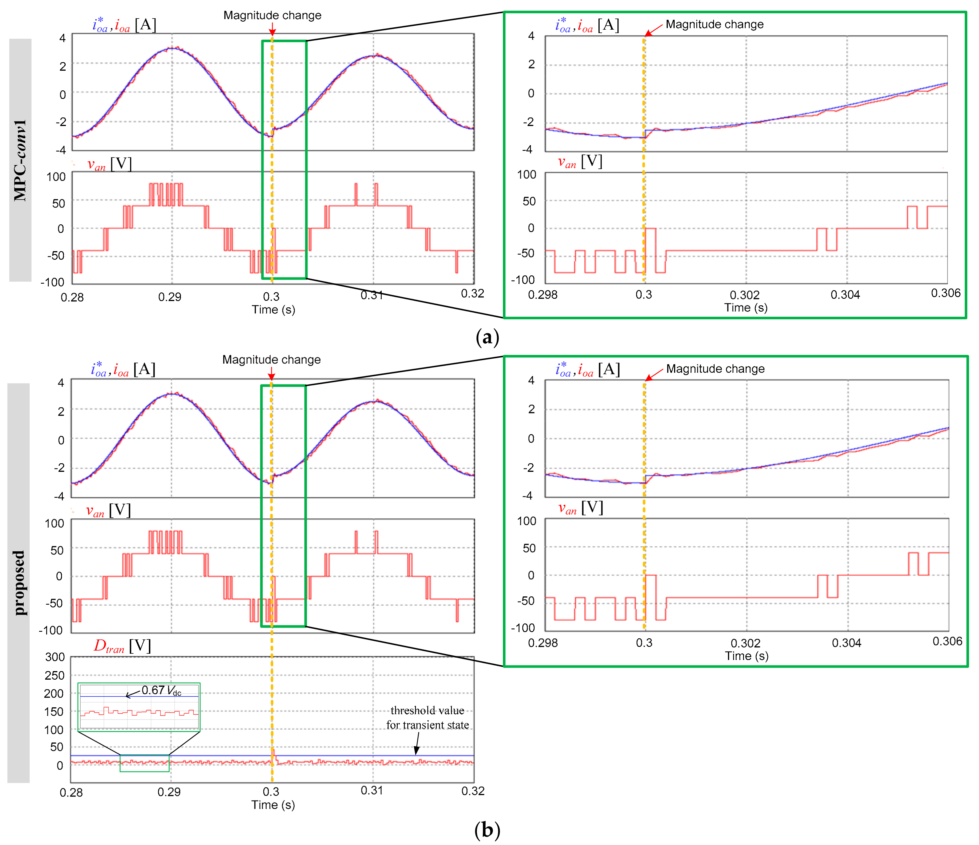
Figure 17.
Simulation waveforms of the a-phase actual current, a-phase reference current, and a-phase inverter phase voltage during the transient state of the reference current change from −3 A to 3 A obtained using (a) the MPC-conv1 method, (b) the proposed method.
Figure 17.
Simulation waveforms of the a-phase actual current, a-phase reference current, and a-phase inverter phase voltage during the transient state of the reference current change from −3 A to 3 A obtained using (a) the MPC-conv1 method, (b) the proposed method.

Figure 18.
Simulation waveforms of the a-phase actual current, a-phase reference current, and a-phase inverter phase voltage during the transient state of the load change from from 20 Ω to 19 Ω obtained using (a) the MPC-conv1 method, (b) the proposed method.
Figure 18.
Simulation waveforms of the a-phase actual current, a-phase reference current, and a-phase inverter phase voltage during the transient state of the load change from from 20 Ω to 19 Ω obtained using (a) the MPC-conv1 method, (b) the proposed method.


Figure 19.
Simulation waveforms of the a-phase actual current, a-phase reference current, and a-phase inverter phase voltage during the transient state of the load change from 20 Ω to 5 Ω obtained using (a) the MPC-conv1 method, (b) the proposed method.
Figure 19.
Simulation waveforms of the a-phase actual current, a-phase reference current, and a-phase inverter phase voltage during the transient state of the load change from 20 Ω to 5 Ω obtained using (a) the MPC-conv1 method, (b) the proposed method.
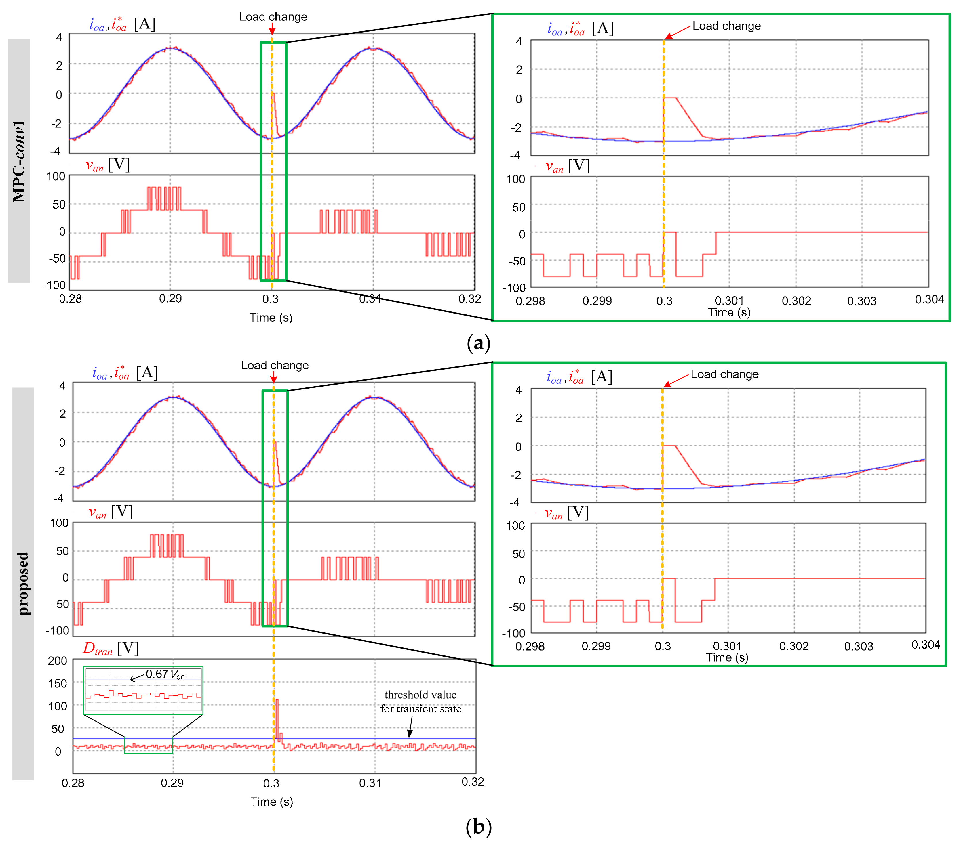
Figure 20.
Simulation waveforms of the a-phase actual current, a-phase reference current, and a-phase inverter phase voltage during the transient state of the changes of the reference current in magnitude from −3 A to −1 A and a 40° phase advance using (a) the MPC-conv1 method, (b) the proposed method.
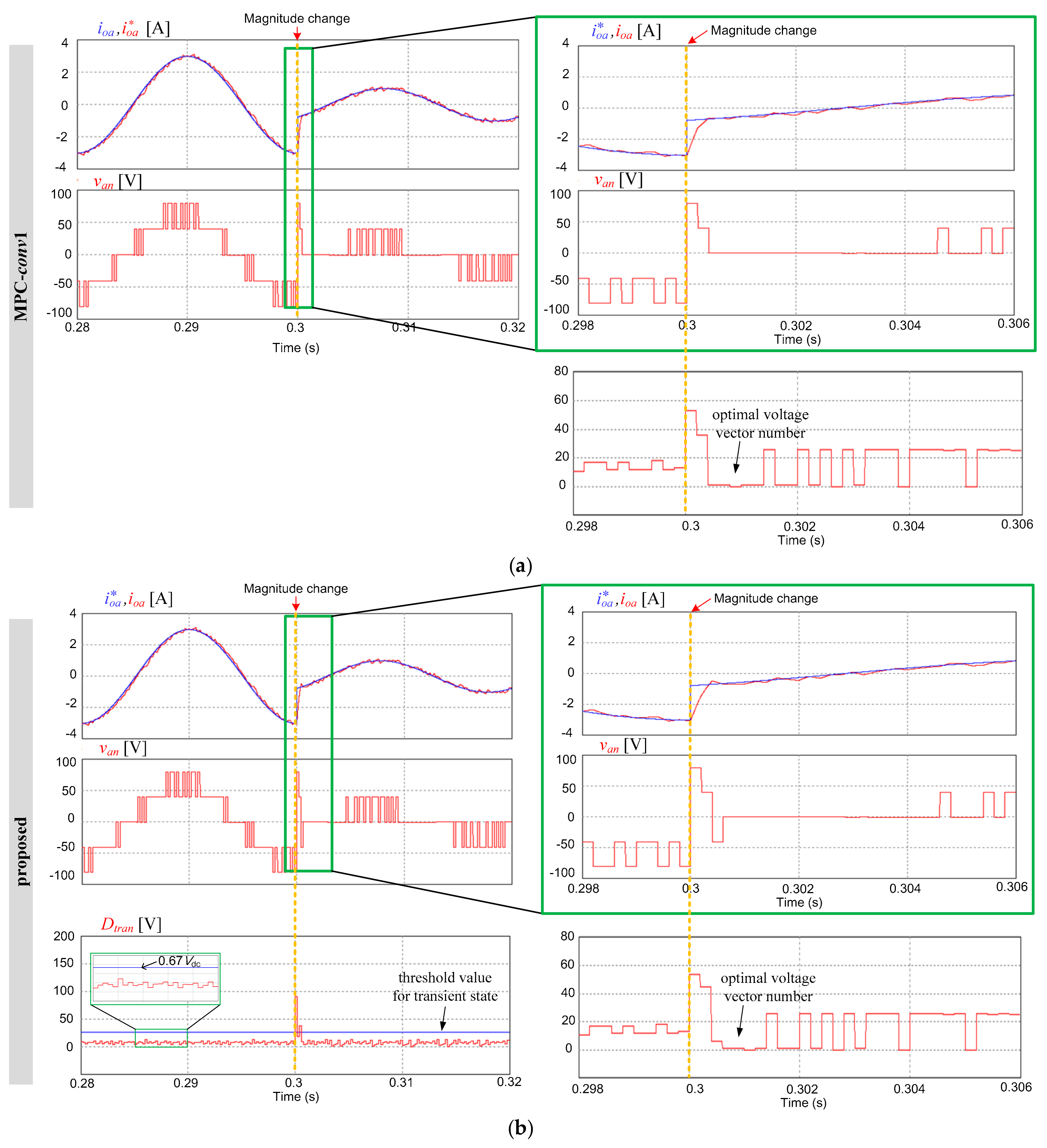
Figure 21.
Simulation waveforms of the a-phase actual current, a-phase reference current, and a-phase inverter-phase voltage during the transient state of the changes of the reference current in magnitude from 3 A to 1 A, and a 40° phase delay using (a) the MPC-conv1 method, (b) the proposed method.
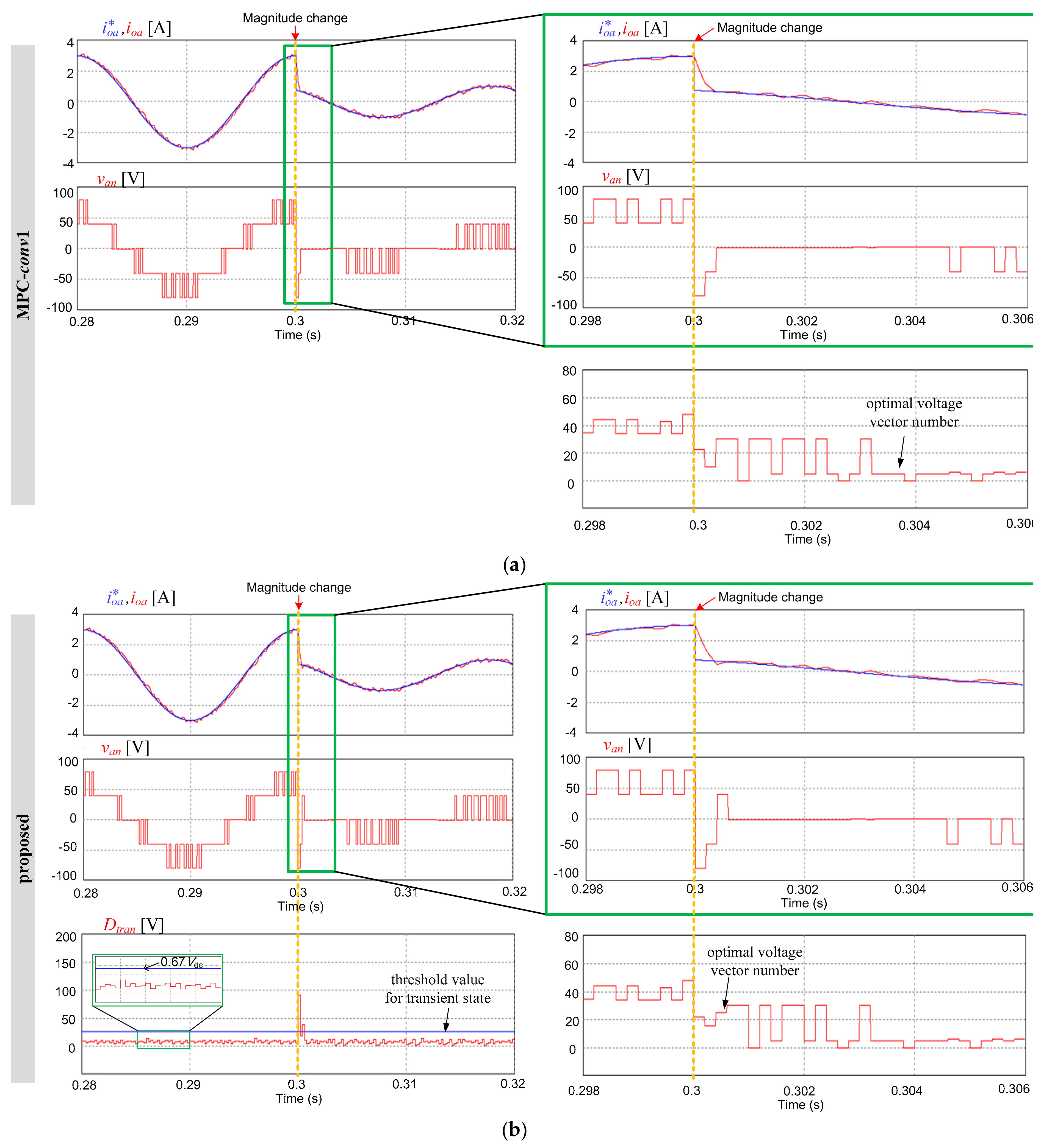
Figure 22.
A five-level CHB inverter. (a) Block diagram of the experimental setup and (b) photograph of the prototype setup.
Figure 22.
A five-level CHB inverter. (a) Block diagram of the experimental setup and (b) photograph of the prototype setup.

Figure 23.
Experimental waveforms of the three-phase load currents (ioa, iob, ioc) and a-phase reference current (), inverter-phase voltage (van), and line–line voltage (vab) during a steady state obtained using the (a) MPC-conv1 method, (b) MPC-conv2 method, (c) proposed method.
Figure 23.
Experimental waveforms of the three-phase load currents (ioa, iob, ioc) and a-phase reference current (), inverter-phase voltage (van), and line–line voltage (vab) during a steady state obtained using the (a) MPC-conv1 method, (b) MPC-conv2 method, (c) proposed method.
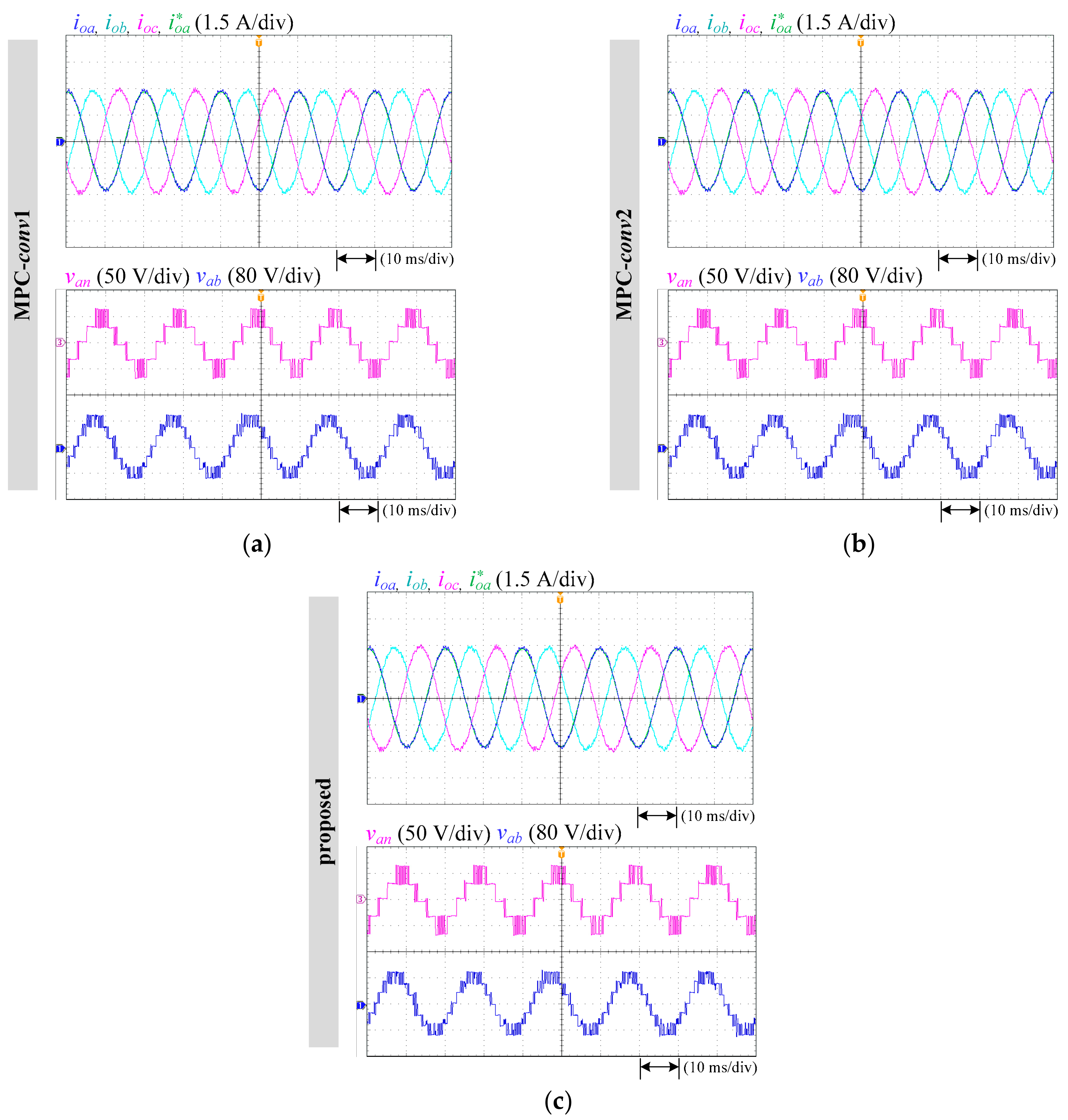
Figure 24.
Experimental waveforms of a-phase load currents (ioa), a-phase reference current (), and a-phase inverter-phase voltage (van) during a transient state of the reference current magnitude change from −3 A to 1.5 A obtained by (a) the MPC-conv1 method, (b) the MPC-conv2 method, (c) the proposed method.
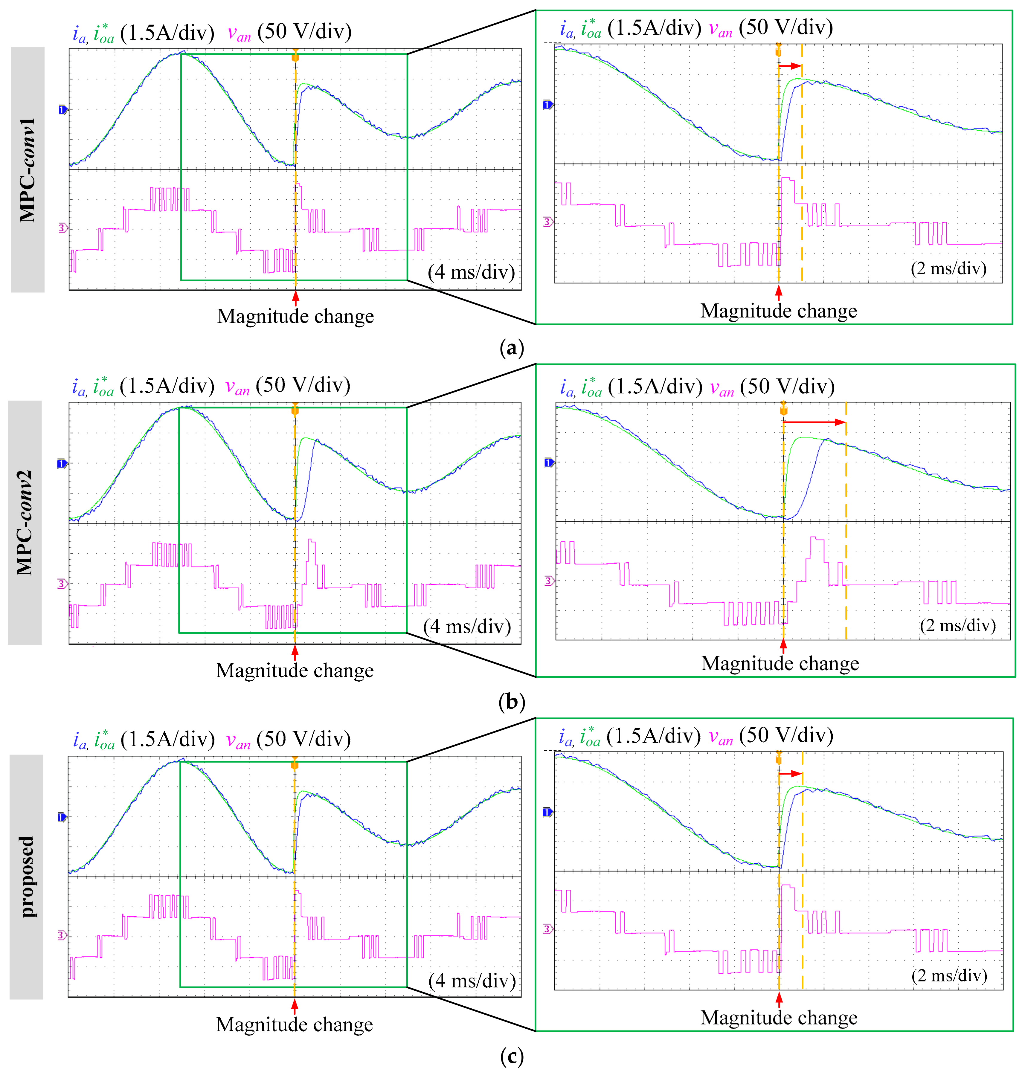
Figure 25.
Experimental waveforms of a-phase load current (ioa), a-phase reference current (), and a-phase inverter phase voltage (van) during a transient state of frequency step-change of the reference currents from 50 Hz to 75 Hz obtained using the (a) MPC-conv1 method, (b) MPC-conv2 method, (c) proposed method.

Table 1.
Relationship of the number of cells, voltage levels, and voltage vectors of the multilevel CHB inverter.
Table 1.
Relationship of the number of cells, voltage levels, and voltage vectors of the multilevel CHB inverter.
| Number of Cell (N) | Voltage Level (M) | Total Vector (Lv) | Non-Redundant Vector (Nnr) |
|---|---|---|---|
| 2 | 5 | 125 | 61 |
| 3 | 7 | 343 | 127 |
| 4 | 9 | 729 | 217 |
| N | 2N + 1 | (2N + 1)3 | 12N2 + 6N + 1 |
Table 2.
Comparative experimental results.
| State | Features | MPC-conv1 | MPC-conv2 | Proposed |
|---|---|---|---|---|
| Steady state | Digital signal processor (DSP) execution times (ms) | 98.92 | 20.17 | 24.73 |
| Reduction rate of DSP time (%) | - | 79.6 | 75 | |
| Transient state | DSP execution times (ms) | 98.92 | 20.17 | 54.12 |
| Reduction rate of DSP time (%) | - | 79.6 | 45.3 | |
| Steady state | Total harmonic distortion (%) | 2.77 | 2.77 | 2.77 |
| Steady state | Mean square error of load current (mA) | 15.2 | 15.2 | 15.2 |
| Transient state | Response time of transients (ms) | 1 | 2.3 | 1 |
© 2018 by the authors. Licensee MDPI, Basel, Switzerland. This article is an open access article distributed under the terms and conditions of the Creative Commons Attribution (CC BY) license (http://creativecommons.org/licenses/by/4.0/).
Share and Cite
MDPI and ACS Style
Chan, R.; Kwak, S. Improved Finite-Control-Set Model Predictive Control for Cascaded H-Bridge Inverters. Energies 2018, 11, 355. https://doi.org/10.3390/en11020355
AMA Style
Chan R, Kwak S. Improved Finite-Control-Set Model Predictive Control for Cascaded H-Bridge Inverters. Energies. 2018; 11(2):355. https://doi.org/10.3390/en11020355
Chicago/Turabian StyleChan, Roh, and Sangshin Kwak. 2018. "Improved Finite-Control-Set Model Predictive Control for Cascaded H-Bridge Inverters" Energies 11, no. 2: 355. https://doi.org/10.3390/en11020355
Note that from the first issue of 2016, this journal uses article numbers instead of page numbers. See further details here.