Optimal Control Algorithms with Adaptive Time-Mesh Refinement for Kite Power Systems

Abstract

This article addresses the problem of optimizing electrical power generation using kite power systems (KPSs). KPSs are airborne wind energy systems that aim to harvest the power of strong and steady high-altitude winds. With the aim of maximizing the total energy produced in a given time interval, we numerically solve an optimal control problem and thereby obtain trajectories and controls for kites. Efficiently solving these optimal control problems is crucial when the results are used in real-time control schemes, such as model predictive control. For this highly nonlinear problem, we derive continuous-time models—in 2D and 3D—and implement an adaptive time-mesh refinement algorithm. By solving the optimal control problem with such an adaptive refinement strategy, we generate a block-structured adapted mesh which gives results as accurate as those computed using fine mesh, yet with much less computing effort and high savings in memory and computing time.

1. Introduction

In the last few years we have seen a fast increase in installed wind power capacity. The installed cumulative power grew by 12.6% in 2016, reaching a total of 486.8 GW [1]. Despite the significant and increasing number of wind farm installations (at low heights), most of the existing wind energy is observed at great heights and is still unexplored. Far from the Earth’s surface, the wind is more powerful and, more importantly, much more consistent. Nevertheless, the conventional wind turbines mounted on towers cannot harvest such winds. To exploit high-altitude winds, a growing number of research groups in Europe and in the U.S. have recently been proposing and developing airborne wind energy systems (AWES), mainly using kites or rigid wing systems. The huge potential of the research in this topic has already been recognized and the economic viability of the concept is starting to be explored by a few start-up companies, including AmpyxPower (the Netherlands, [2]), KiteGen (Italy, [3]), KitePower (the Netherlands), and Makani Power (now part of Google X, USA, [4]), to name a few. In Portugal, Omnidea [5] has been developing an AWES based on the Magnus effect. Overviews of AWES research and technologies are given in [6,7,8].

Most of the systems being developed are based on exploiting the powerful crosswind kite power described by Loyd in 1980 [9]. These systems use the fact that aerodynamic lift is proportional to the square of the (apparent) wind velocity

$${\overrightarrow{\mathrm{F}}}^{\mathrm{lift}}=\raisebox{1ex}{$1$}\!\left/ \!\raisebox{-1ex}{$2$}\right.c_{\mathrm{L}}\left(\alpha \right)A{\mathbf{v}}_a^2.$$

Therefore, maximum power extraction occurs when the kite is flying at high speeds in a plane orthogonal to the wind direction (the kite behaves much like the tip of the blade in a turbine). In kite power systems with a generator on the ground, the generation of electrical power is done using a controlled kite (tethered wing) by unwinding a cable coiled around a drum connected to a generator. Energy is generated when the cable is unwinding. However, since the length of the cable is finite, eventually the cable has to be coiled back. Power is consumed when coiling back the cable, but the whole cycle is done in such a way that the balance—the total energy produced—is positive.

We consider the optimal control problem with a continuous-time model of the kite power system, further developing the work reported in [10,11]. The solution to this problem provides the trajectory of the kite and the corresponding control laws that maximize the total energy produced in a given time interval. The efficient solution of optimal control problems is necessary so that the results may be used in a real-time control schemes such as model predictive control (see e.g., [12,13,14,15]). We solve this problem in a time-mesh that is adaptively refined to achieve a desired level of accuracy. The adaptive mesh refinement (AMR) strategy used considers, in the optimal control problem (OCP) context, several refinement criteria in a multi-level scheme [16]. A major feature of the strategy is to consider the local error of the dual variables as a refinement criterion. This error can be computed efficiently by comparing the solution of a linear differential equation system—the adjoint equation of the maximum principle—with the numerically obtained multipliers.

Details of this technique and its use in other nonlinear systems are reported in [16,17]. The refinement strategy resulted in higher accuracy levels with a lower overall computational time when compared with the use of traditional meshes with equidistant spacing in the continuous-time OCP, and with a priori discretized versions of the OCP. In particular, the time to obtain a solution with a similar level of accuracy represented 4% to 30% of the time needed using traditional equidistant meshes. The benefits of using an adaptive time mesh are particularly more evident in highly nonlinear systems, as is the case of the controlled kite and other nonholonomic systems. The technique led to the use of finer meshes in time intervals where sharp turns of the kite occur. A simplified problem in two dimensions was solved with the AMR 29 times faster than with an equidistant mesh leading to the same level of accuracy. The complete 3D problem was successfully solved using the AMR strategy, while when using an equidistant mesh leading to the same level of accuracy, the maximum number of iterations of the nonlinear optimization solver was exceeded.

2. Kite Power System Model

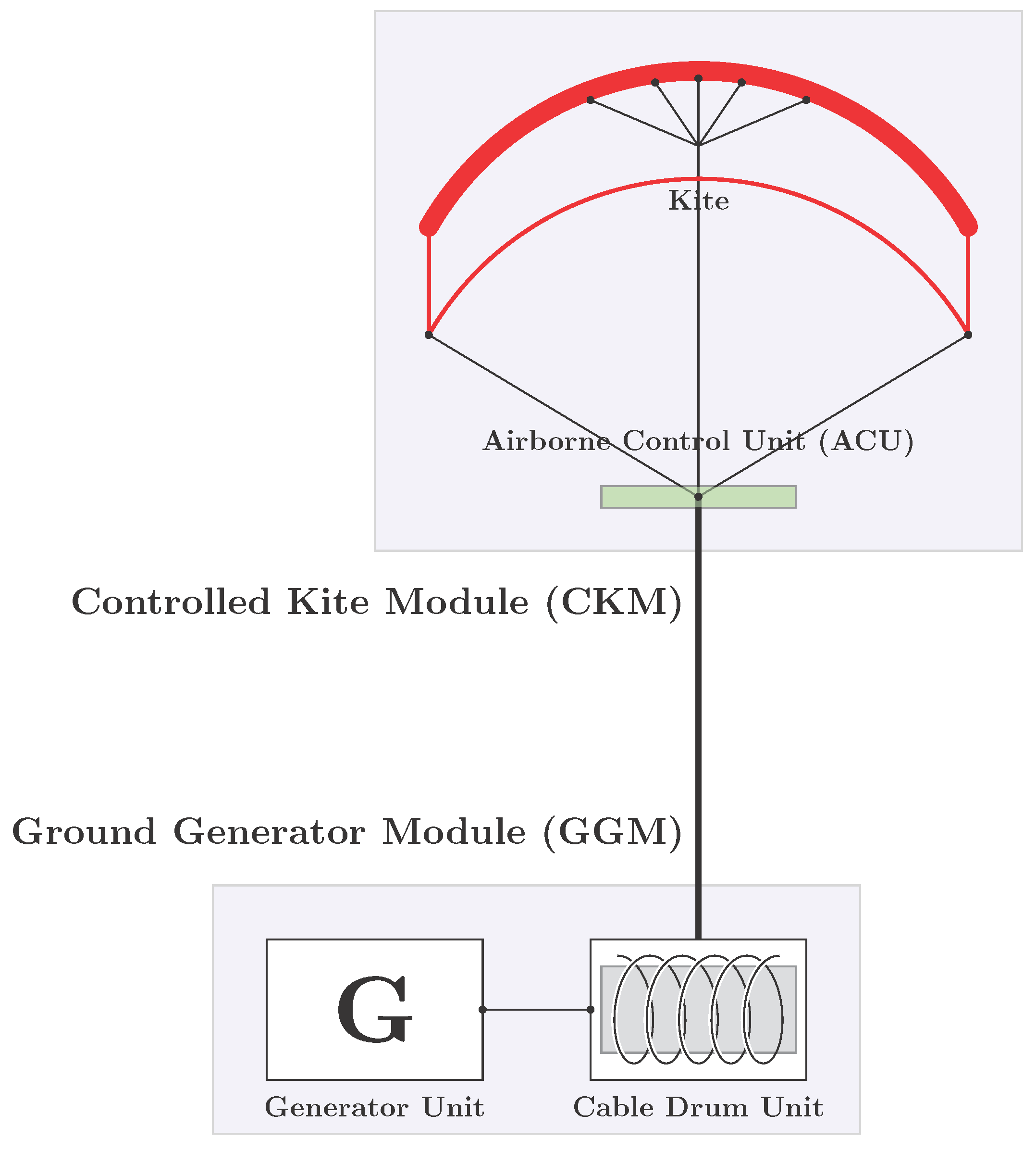
The AWES considered in the paper is a kite generator system (KGS) involving a controlled kite module (CKM) connected to a ground generator module (GGM) by a single tether (see Figure 1). Among the recent AWES proposals, the KGS type is one of the most simple, yet appears to be one of the most promising. One of its main advantages is having the generator on the ground, reducing not only safety risks but also the building costs since it does not require heavy infrastructures. The CKM comprises the kite and the airborne control unit (ACU) while the GGM comprises the generator unit and the cable drum unit.

There is a single tether going from the GGM to the ACU and the line tension in the described models below refers to the tension in this single tether. From the ACU to the kite, three or more lines are attached. The main line, which takes most of the load, is attached to the leading edge of the kite in a bridle configuration. The other two lines attached to each corner of the trailing edge are used to control the roll angle ($\psi$) and angle of attack ($\alpha$). By pulling both of these lines we increase the angle of attack and a differential pull in these lines controls the roll of the kite.

2.1. 2D Kite Model

We start by addressing a simplified 2D model of a kite power system moving in a vertical plane containing the wind vector. We consider two coordinate systems:

Global G: 

A Cartesian coordinate system $(x,z)$ where x is aligned according to the wind direction ${\mathbf{v}}_w=(v_w,0)$− basis $({\overrightarrow{\mathbf{e}}}_x,{\overrightarrow{\mathbf{e}}}_z)$,

Local L: 

A polar coordinate system $(r,\beta )$ centred at the kite position—basis $({\overrightarrow{\mathbf{e}}}_r,{\overrightarrow{\mathbf{e}}}_{\beta })$.

Considering the position of the kite $\left(\mathbf{p}\right)$

$$\mathbf{p}=\left[\begin{array}{c}rcos\left(\beta \right)\\ rsin\left(\beta \right)\end{array}\right]$$

we get

$${\overrightarrow{\mathbf{e}}}_r={\displaystyle \frac{{\displaystyle \frac{\partial \mathbf{p}}{\partial r}}}{\left|{\displaystyle \frac{\partial \mathbf{p}}{\partial r}}\right|}}=\left[\begin{array}{c}cos\left(\beta \right)\\ sin\left(\beta \right)\end{array}\right]\mathrm{and}{\overrightarrow{\mathbf{e}}}_{\beta }={\displaystyle \frac{{\displaystyle \frac{\partial \mathbf{p}}{\partial \beta }}}{\left|{\displaystyle \frac{\partial \mathbf{p}}{\partial \beta }}\right|}}=\left[\begin{array}{c}-sin\left(\beta \right)\\ cos\left(\beta \right)\end{array}\right],$$

and, therefore, the rotation matrix from $\mathrm{L}$ coordinate system to $\mathrm{G}$ is

$${\mathrm{R}}_{\mathrm{L}\mathrm{G}}=\left[\begin{array}{cc}{\overrightarrow{\mathbf{e}}}_r& {\overrightarrow{\mathbf{e}}}_{\beta }\end{array}\right]=\left[\begin{array}{cc}cos\left(\beta \right)& -sin\left(\beta \right)\\ sin\left(\beta \right)& cos\left(\beta \right)\end{array}\right]$$

and the rotation matrix from $\mathrm{G}$ coordinate system to $\mathrm{L}$ is ${\mathrm{R}}_{\mathrm{G}\mathrm{L}}={\mathrm{R}}_{\mathrm{L}\mathrm{G}}^{-1}={\mathrm{R}}_{\mathrm{L}\mathrm{G}}^{\top }$.

2.2. Acting Forces

Considering the mass of the kite $\left(m\right)$ and the total force acting on it $\left(\mathrm{F}\right)$, Newton’s law reads

$$m\ddot{\mathbf{p}}=\mathrm{F}.$$

(1)

In (1) $\mathrm{F}$ can be decomposed into tether tension at the ground $({\overrightarrow{\mathrm{F}}}^{\mathrm{th}})$, gravity $({\overrightarrow{\mathrm{F}}}^{\mathrm{grav}})$, and aerodynamic force $({\overrightarrow{\mathrm{F}}}^{\mathrm{aer}}\left(\alpha \right))$, i.e.,

$$\mathrm{F}={\overrightarrow{\mathrm{F}}}^{\mathrm{th}}+{\overrightarrow{\mathrm{F}}}^{\mathrm{grav}}+{\overrightarrow{\mathrm{F}}}^{\mathrm{aer}}\left(\alpha \right).$$

(2)

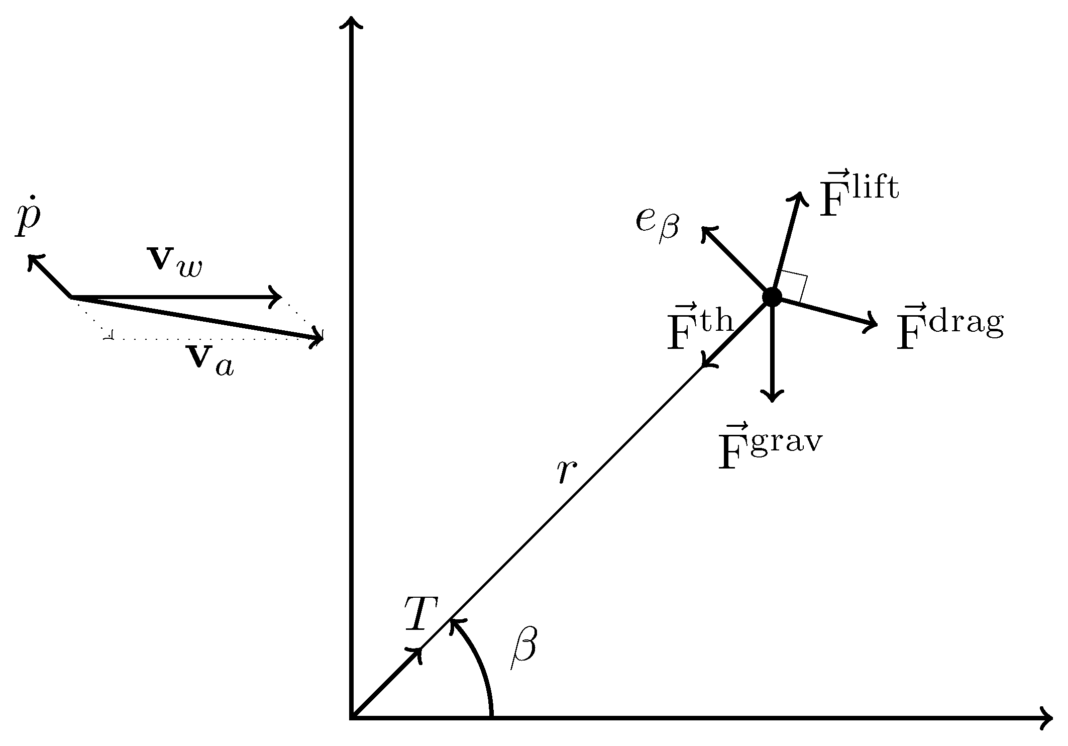
The tether force is completely aligned with the first coordinate of the local coordinate system while the kite gravitational force is completely aligned with the last coordinate of the global coordinate system (see Figure 2).

$$\begin{array}{cc}\hfill {\overrightarrow{\mathrm{F}}}^{\mathrm{th}}& =-T{\overrightarrow{\mathbf{e}}}_r={\left[\begin{array}{c}-T\\ 0\end{array}\right]}_{\mathrm{L}}\hfill \\ \hfill {\overrightarrow{\mathrm{F}}}^{\mathrm{grav}}& =-mg{\overrightarrow{\mathbf{e}}}_z={\left[\begin{array}{c}0\\ -mg\end{array}\right]}_{\mathrm{G}}={\left[\begin{array}{c}-mgsin\left(\beta \right)\\ -mgcos\left(\beta \right)\end{array}\right]}_{\mathrm{L}}\hfill \end{array}$$

We consider the case in which the drag force is aligned with the apparent wind velocity and the lift force has its upward normal direction (see Figure 2).

$${\overrightarrow{\mathrm{F}}}^{\mathrm{aer}}\left(\alpha \right)={\overrightarrow{\mathrm{F}}}^{\mathrm{lift}}\left(\alpha \right)+{\overrightarrow{\mathrm{F}}}^{\mathrm{drag}}\left(\alpha \right)$$

where

$$\begin{array}{cc}\hfill {\overrightarrow{\mathrm{F}}}^{\mathrm{drag}}\left(\alpha \right)& =\raisebox{1ex}{$1$}\!\left/ \!\raisebox{-1ex}{$2$}\right.\rho A{c}_{\mathrm{D}}\left(\alpha \right)\parallel {\mathbf{v}}_a\parallel {\mathbf{v}}_a\hfill \\ \hfill {\overrightarrow{\mathrm{F}}}^{\mathrm{lift}}\left(\alpha \right)& =\raisebox{1ex}{$1$}\!\left/ \!\raisebox{-1ex}{$2$}\right.\rho A{c}_{\mathrm{L}}\left(\alpha \right)\parallel {\mathbf{v}}_a\parallel {\mathrm{R}}_{90}{\mathbf{v}}_a\hfill \end{array}$$

where ${\mathrm{R}}_{90}$ is the 90° anticlockwise rotation matrix. Thus

$${\overrightarrow{\mathrm{F}}}^{\mathrm{aer}}\left(\alpha \right)=\left[\begin{array}{c}{\mathrm{F}}_r^{aer}\left(\alpha \right)\\ {\mathrm{F}}_{\beta }^{aer}\left(\alpha \right)\end{array}\right]=\raisebox{1ex}{$1$}\!\left/ \!\raisebox{-1ex}{$2$}\right.\rho A\parallel {\mathbf{v}}_a\parallel \left(c_{\mathrm{D}}\left(\alpha \right){\mathbf{v}}_a+c_{\mathrm{L}}\left(\alpha \right){\mathrm{R}}_{90}{\mathbf{v}}_a\right).$$

In a polar coordinate system

$$\begin{array}{cc}\hfill \dot{\mathbf{p}}& =\dot{r}{\overrightarrow{\mathbf{e}}}_r+r\dot{\beta }{\overrightarrow{\mathbf{e}}}_{\beta }={\left[\begin{array}{c}\dot{r}\\ r\dot{\beta }\end{array}\right]}_{\mathrm{L}}\hfill \end{array}$$

(3)

and

$$\begin{array}{cc}\hfill \ddot{\mathbf{p}}& =\left(\ddot{r}-r{\dot{\beta }}^2\right){\overrightarrow{\mathbf{e}}}_r+(r\ddot{\beta }+2\dot{r}\dot{\beta }){\overrightarrow{\mathbf{e}}}_{\beta }\hfill \\ & ={\left[\begin{array}{c}\ddot{r}-r{\dot{\beta }}^2\\ r\ddot{\beta }+2\dot{r}\dot{\beta }\end{array}\right]}_{\mathrm{L}}={\left[\begin{array}{c}\ddot{r}\\ r\ddot{\beta }\end{array}\right]}_{\mathrm{L}}+\underset{-\raisebox{1ex}{$1$}\!\left/ \!\raisebox{-1ex}{$m$}\right.{\overrightarrow{\mathrm{F}}}^{\mathrm{inert}}}{\underbrace{{\left[\begin{array}{c}-r{\dot{\beta }}^2\\ 2\dot{r}\dot{\beta }\end{array}\right]}_{\mathrm{L}}}}\hfill \end{array}$$

(4)

where ${\overrightarrow{\mathrm{F}}}^{\mathrm{inert}}$ represents the inertial force

$${\overrightarrow{\mathrm{F}}}^{\mathrm{inert}}=m{\left[\begin{array}{c}r{\dot{\beta }}^2\\ -2\dot{r}\dot{\beta }\end{array}\right]}_{\mathrm{L}}.$$

Considering the aerodynamic force directions defined by the apparent wind, we can write

$$\begin{array}{cc}\hfill m\left[\begin{array}{c}\ddot{r}\\ r\ddot{\beta }\end{array}\right]& ={\overrightarrow{\mathrm{F}}}^{\mathrm{th}}+{\overrightarrow{\mathrm{F}}}^{\mathrm{grav}}+{\overrightarrow{\mathrm{F}}}^{\mathrm{aer}}+{\overrightarrow{\mathrm{F}}}^{\mathrm{inert}}\hfill \\ & =\left[\begin{array}{c}-T\\ 0\end{array}\right]-mg\left[\begin{array}{c}sin\left(\beta \right)\\ cos\left(\beta \right)\end{array}\right]+\left[\begin{array}{c}{\mathrm{F}}_r^{aer}\left(\alpha \right)\\ {\mathrm{F}}_{\beta }^{aer}\left(\alpha \right)\end{array}\right]+m\left[\begin{array}{c}r{\dot{\beta }}^2\\ -2\dot{r}\dot{\beta }\end{array}\right]\hfill \end{array}$$

and therefore,

$$\begin{array}{cc}\hfill \left[\begin{array}{c}\ddot{r}\\ \ddot{\beta }\end{array}\right]& ={\displaystyle \frac{1}{m}}\left[\begin{array}{c}-T-gmsin\left(\beta \right)+{\mathrm{F}}_r^{aer}\left(\alpha \right)+mr{\dot{\beta }}^2\\ \raisebox{1ex}{$1$}\!\left/ \!\raisebox{-1ex}{$r$}\right.\left(-gmcos\left(\beta \right)+{\mathrm{F}}_{\beta }^{aer}\left(\alpha \right)-2m\dot{r}\dot{\beta }\right)\end{array}\right].\hfill \end{array}$$

Considering $\dot{r}=v_t\in \mathbb{R}$, we have $\ddot{r}=0$ and therefore we can define the state $\mathbf{x}=\left(r,\beta ,\dot{\beta }\right)$, the control $\mathbf{u}=\left(v_t,\alpha \right)$, and the dynamic equation

$$\begin{array}{cc}\hfill \dot{\mathbf{x}}& =\left[\begin{array}{c}{v}_t\\ \dot{\beta }\\ {\displaystyle \frac{1}{mr}}\left(-gmcos\left(\beta \right)+{\mathrm{F}}_{\beta }^{aer}\left(\alpha \right)-2m\dot{r}\dot{\beta }\right)\end{array}\right]:=\mathbf{f}(\mathbf{x},\mathbf{u}).\hfill \end{array}$$

(5)

2.3. 3D Model

We model the forces acting on the kite in a spherical coordinate system positioned at the center of the kite, similarly to [18,19]. We consider three coordinate systems:

Global G: 

An inertial Cartesian coordinate system $(x,y,z)$ where the origin is on the ground at the point of attachment of the tether and x is aligned according to the wind direction ${\mathbf{v}}_w=(v_w,0,0)$, on the basis of $({\overrightarrow{\mathbf{e}}}_x,{\overrightarrow{\mathbf{e}}}_y,{\overrightarrow{\mathbf{e}}}_z)$.

We consider that the kite is positioned in a point $\mathbf{p}$ with coordinates $(x,y,z)$.

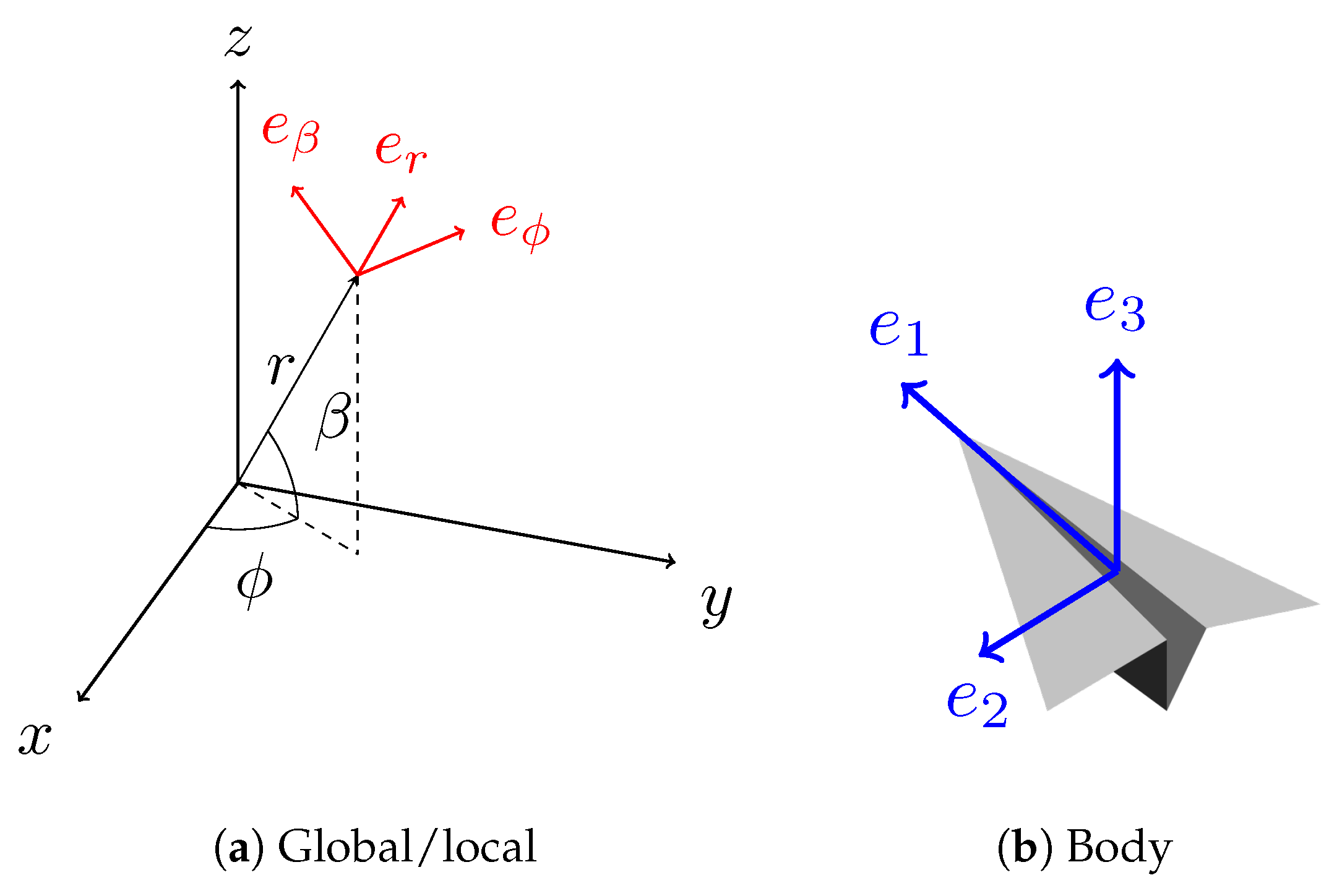
Local L: 

A non-inertial spherical coordinate system $(r,\varphi ,\beta )$ on the basis of $({\overrightarrow{\mathbf{e}}}_r,{\overrightarrow{\mathbf{e}}}_{\varphi },{\overrightarrow{\mathbf{e}}}_{\beta })$ (Figure 3a).

Body B: 

A non-inertial Cartesian coordinate system attached to the kite body on the basis of $({\overrightarrow{\mathbf{e}}}_1,{\overrightarrow{\mathbf{e}}}_2,{\overrightarrow{\mathbf{e}}}_3)$. ${\overrightarrow{\mathbf{e}}}_1$ coincides with the kite’s longitudinal axis pointing forward, ${\overrightarrow{\mathbf{e}}}_2$ in the kite transversal axis points to the left wing tip, and ${\overrightarrow{\mathbf{e}}}_3$ in the kite vertical axis points upwards (Figure 3b).

Considering the position

$$\mathbf{p}=\left[\begin{array}{c}x\\ y\\ z\end{array}\right]=\left[\begin{array}{c}rcos\left(\beta \right)cos\left(\varphi \right)\\ rcos\left(\beta \right)sin\left(\varphi \right)\\ rsin\left(\beta \right)\end{array}\right],$$

the rotation matrix from $\mathrm{L}$ coordinate system to $\mathrm{G}$ is

$${\mathrm{R}}_{\mathrm{L}\mathrm{G}}=\left[\begin{array}{ccc}{\overrightarrow{\mathbf{e}}}_r& {\overrightarrow{\mathbf{e}}}_{\varphi }& {\overrightarrow{\mathbf{e}}}_{\beta }\end{array}\right]=\left[\begin{array}{ccc}cos\left(\beta \right)cos\left(\varphi \right)& -sin\left(\varphi \right)& -sin\left(\beta \right)cos\left(\varphi \right)\\ cos\left(\beta \right)sin\left(\varphi \right)& cos\left(\varphi \right)& -sin\left(\beta \right)sin\left(\varphi \right)\\ sin\left(\beta \right)& 0& cos\left(\beta \right)\end{array}\right],$$

and the rotation matrix from $\mathrm{G}$ coordinate system to $\mathrm{L}$ is ${\mathrm{R}}_{\mathrm{G}\mathrm{L}}={\mathrm{R}}_{\mathrm{L}\mathrm{G}}^{-1}={\mathrm{R}}_{\mathrm{L}\mathrm{G}}^{\top }$.

We consider the apparent wind velocity ${\mathbf{v}}_a={\mathbf{v}}_w-\dot{\mathbf{p}}.$ Assume that its radial component ${\mathbf{v}}_{a,r}$ is always strictly positive and that the kite body is at all times positioned in such a way that its longitudinal axis is aligned with the apparent wind velocity, that is ${\overrightarrow{\mathbf{e}}}_1=-{\mathbf{v}}_a/\parallel {\mathbf{v}}_a\parallel .$ Let $\psi$ be the roll angle measuring rotation around the ${\overrightarrow{\mathbf{e}}}_1$ axis. We consider that ${\tilde{\mathbf{e}}}_2={\overrightarrow{\mathbf{e}}}_2$ is initially(for $\psi =0$) in the plane $\tau$, tangent to a sphere centred at the origin (containing the axis ${\overrightarrow{\mathbf{e}}}_{\varphi }$ and ${\overrightarrow{\mathbf{e}}}_{\beta }$). We have that ${\tilde{\mathbf{e}}}_2\perp {\overrightarrow{\mathbf{e}}}_r,and{\tilde{\mathbf{e}}}_2\perp {\overrightarrow{\mathbf{e}}}_1.$ We can then define ${\displaystyle {\tilde{\mathbf{e}}}_2=\frac{{\overrightarrow{\mathbf{e}}}_r\times {\overrightarrow{\mathbf{e}}}_1}{\parallel {\overrightarrow{\mathbf{e}}}_r\times {\overrightarrow{\mathbf{e}}}_1\parallel }.}$ Finally, we consider the kite body has an anti-clockwise rotation of $\psi$ around the ${\overrightarrow{\mathbf{e}}}_1$ axis: the roll angle. We assume that the roll angle $\psi$ can be controlled directly. In fact, since the kite has some mass, the roll angle cannot be selected arbitrarily at each instant. We would have to control the angular acceleration and thereby the angular velocity and roll angle. However, since the rotation of the kite is much faster than its translational movement in the defined operational range, we can consider, as a simplification, that the roll angle is a directly actuated control variable. For example, in a two-line kite where d is the distance between attachment points and $\Delta r$ is the relative difference between the lengths of each line, we have $sin\psi =\Delta r/d$ (cf. [19]). Using Rodrigues’ formula to rotate ${\tilde{\mathbf{e}}}_2$ by $\psi$ around ${\overrightarrow{\mathbf{e}}}_1$, we obtain

$${\overrightarrow{\mathbf{e}}}_2={\tilde{\mathbf{e}}}_{2}cos\psi +({\overrightarrow{\mathbf{e}}}_1\times {\tilde{\mathbf{e}}}_2)sin\psi +{\overrightarrow{\mathbf{e}}}_1({\overrightarrow{\mathbf{e}}}_1·{\tilde{\mathbf{e}}}_2)(1-cos\psi )$$

(6)

and finally, we define ${\overrightarrow{\mathbf{e}}}_3$ forming a right-handed coordinate system ${\overrightarrow{\mathbf{e}}}_3={\overrightarrow{\mathbf{e}}}_1\times {\overrightarrow{\mathbf{e}}}_2.$

As before, the total force acting on it can be decomposed as

$$m\ddot{\mathbf{p}}={\overrightarrow{\mathrm{F}}}^{\mathrm{th}}+{\overrightarrow{\mathrm{F}}}^{\mathrm{grav}}+{\overrightarrow{\mathrm{F}}}^{\mathrm{aer}}\left(\alpha \right)$$

(7)

where

$$\begin{array}{cc}\hfill {\overrightarrow{\mathrm{F}}}^{\mathrm{th}}& =-T{\overrightarrow{\mathbf{e}}}_r={\left[\begin{array}{c}-T\\ 0\\ 0\end{array}\right]}_{\mathrm{L}},\hfill \\ \hfill {\overrightarrow{\mathrm{F}}}^{\mathrm{grav}}& =-mg{\overrightarrow{\mathbf{e}}}_z={\left[\begin{array}{c}0\\ 0\\ -mg\end{array}\right]}_{\mathrm{G}}={\left[\begin{array}{c}-mgsin\beta \\ 0\\ -mgcos\beta \end{array}\right]}_{\mathrm{L}},\hfill \\ \hfill {\overrightarrow{\mathrm{F}}}^{\mathrm{aer}}\left(\alpha \right)& =\raisebox{1ex}{$1$}\!\left/ \!\raisebox{-1ex}{$2$}\right.\rho A{\parallel {\mathbf{v}}_a\parallel }^2(c_{\mathrm{L}}\left(\alpha \right){\overrightarrow{\mathbf{e}}}_3-c_{\mathrm{D}}\left(\alpha \right){\overrightarrow{\mathbf{e}}}_1).\hfill \end{array}$$

In the local coordinate system

$$\begin{array}{cc}\hfill \ddot{\mathbf{p}}& ={\left[\begin{array}{c}\ddot{r}\\ r\ddot{\varphi }cos\left(\beta \right)\\ r\ddot{\beta }\end{array}\right]}_{\mathrm{L}}+\underset{-\raisebox{1ex}{$1$}\!\left/ \!\raisebox{-1ex}{$m$}\right.{\overrightarrow{\mathrm{F}}}^{\mathrm{inert}}}{\underbrace{{\left[\begin{array}{c}-r{\dot{\beta }}^2-r{\dot{\varphi }}^2{cos}^2\left(\beta \right)\\ 2\dot{r}\dot{\varphi }cos\left(\beta \right)-2r\dot{\varphi }\dot{\beta }sin\left(\beta \right)\\ 2\dot{r}\dot{\beta }+r{\dot{\varphi }}^{2}cos\left(\beta \right)sin\left(\beta \right)\end{array}\right]}_{\mathrm{L}}}}\hfill \end{array}$$

(8)

where the second term is $-\raisebox{1ex}{$1$}\!\left/ \!\raisebox{-1ex}{$m$}\right.{\overrightarrow{\mathrm{F}}}^{\mathrm{inert}}$ with ${\overrightarrow{\mathrm{F}}}^{\mathrm{inert}}$ representing the inertial forces (centrifugal and Coriolis) in the local coordinate system.

Now, we can write

$$\begin{array}{cc}\hfill m\left[\begin{array}{c}\ddot{r}\\ r\ddot{\varphi }cos\left(\beta \right)\\ r\ddot{\beta }\end{array}\right]& ={\overrightarrow{\mathrm{F}}}^{\mathrm{th}}+{\overrightarrow{\mathrm{F}}}^{\mathrm{grav}}+{\overrightarrow{\mathrm{F}}}^{\mathrm{aer}}\left(\alpha \right)+{\overrightarrow{\mathrm{F}}}^{\mathrm{inert}}\hfill \end{array}$$

(9)

We assume that the tether acceleration $\ddot{r}$ can be controlled directly by $a_t$. Denoting by T the tension on the tether at the base, we have $T={\mathrm{F}}_r-m{a}_t.$ Defining the state $\mathbf{x}=(r,\varphi ,\beta ,\dot{r},\dot{\varphi },\dot{\beta })$ and the control $\mathbf{u}=\left(a_t,\alpha ,\psi \right)$, the dynamic equation is

$$\dot{\mathbf{x}}\left(t\right)=f(\mathbf{x}\left(t\right),\mathbf{u}\left(t\right))={\displaystyle \frac{\mathrm{d}}{\mathrm{d}t}}\left[\begin{array}{c}r\\ \varphi \\ \beta \\ \dot{r}\\ \dot{\varphi }\\ \dot{\beta }\end{array}\right]=\left[\begin{array}{c}\dot{r}\\ \dot{\varphi }\\ \dot{\beta }\\ a_t\\ {\displaystyle \frac{1}{mrcos\left(\beta \right)}}{\mathrm{F}}_{\varphi }\\ {\displaystyle \frac{1}{mr}}{\mathrm{F}}_{\beta }\end{array}\right].$$

(10)

3. Optimal Control Problem

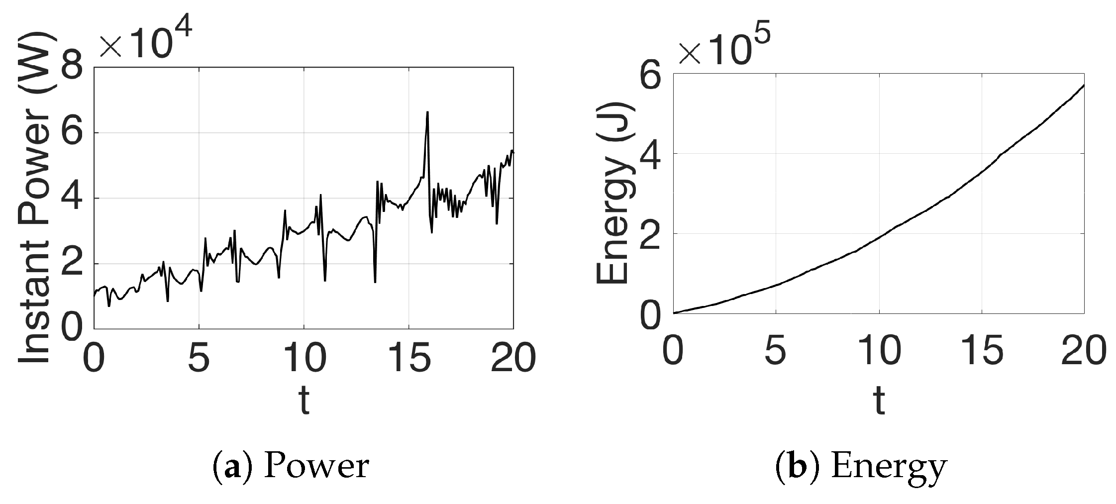
We consider the problem of optimizing power production in a given time period $[t_0,t_f]$ (see e.g., [20,21,22] for a reference on optimal control and on the corresponding numerical methods). The instant power production is given by $P\left(t\right)=\dot{r}T$ and the energy in the interval is

$$E\left(t_f\right)=\underset{t_0}{\overset{t_f}{\int }}P\left(t\right)\mathrm{d}t.$$

(11)

We consider two problems:

($P_1$):

The production cycle, when the terminal state is free;

($P_2$):

The reel-out and reel-in cycle, by imposing that the terminal state should be near the initial one: $\left|\right|\mathbf{x}\left(t_f\right)-\mathbf{x}\left(t_0\right)\left|\right|<\epsilon$.

Considering $t\in [t_0,t_f]$, the problem $\left(P_1\right)$ can be stated as:

$$\mathrm{Maximize}\underset{t_0}{\overset{t_f}{\int }}\dot{r}T\mathrm{d}\mathrm{t}$$

(12)

subject to dynamic constraints

$$\begin{array}{ccccc}\dot{\mathbf{x}}\left(t\right)=\mathbf{f}(\mathbf{x},\mathbf{u})\hfill & & & & \hfill \mathrm{a}.\mathrm{e}.t\in [t_0,t_f]\end{array}$$

input constraints

$$\begin{array}{ccccc}{a}_{min}\le a_t\left(t\right)\le a_{max}\hfill & & & & \hfill \mathrm{a}.\mathrm{e}.t\in [t_0,t_f]\\ {\alpha }_{min}\le \alpha \left(t\right)\le {\alpha }_{max}\hfill & & & & \hfill \mathrm{a}.\mathrm{e}.t\in [t_0,t_f]\\ {\psi }_{min}\le \psi \left(t\right)\le {\psi }_{max}\hfill & & & & \hfill \mathrm{a}.\mathrm{e}.t\in [t_0,t_f]\end{array}$$

the left end-point constraint

$$\begin{array}{cc}\hfill \mathbf{x}\left(t_0\right)& ={\mathbf{x}}_0=(r_0,{\varphi }_0,{\beta }_0,\dot{r_0},\dot{{\varphi }_0},\dot{{\beta }_0})\hfill \end{array}$$

and bounded-state constraints

$$\begin{array}{ccccc}{r}_{min}\le r\left(t\right)\le r_{max}\hfill & & & & \hfill \forall t\in [t_0,t_f]\\ {\varphi }_{min}\le \varphi \left(t\right)\le {\varphi }_{max}\hfill & & & & \hfill \forall t\in [t_0,t_f]\\ {\beta }_{min}\le \beta \left(t\right)\le {\beta }_{max}\hfill & & & & \hfill \forall t\in [t_0,t_f]\end{array}$$

In $\left(P_2\right)$, in order to concentrate the production in the beginning of the time interval, we change the objective function to $e^{-t}\dot{r}T,$ and thus, this problem can be stated as follows:

$$\begin{array}{cc}\hfill \mathrm{Maximize}& \underset{t_0}{\overset{t_f}{\int }}{e}^{-t}\dot{r}T\mathrm{d}\mathrm{t}\hfill \\ \hfill \mathrm{subject}\mathrm{to}\\ & \dot{\mathbf{x}}\left(t\right)=\mathbf{f}(\mathbf{x},\mathbf{u})\hfill & \hfill \mathrm{a}.\mathrm{e}.t\in [t_0,t_f]\\ & a_{min}\le a_t\left(t\right)\le a_{max}\hfill & \hfill \mathrm{a}.\mathrm{e}.t\in [t_0,t_f]\\ & {\alpha }_{min}\le \alpha \left(t\right)\le {\alpha }_{max}\hfill & \hfill \mathrm{a}.\mathrm{e}.t\in [t_0,t_f]\\ & {\psi }_{min}\le \psi \left(t\right)\le {\psi }_{max}\hfill & \hfill \mathrm{a}.\mathrm{e}.t\in [t_0,t_f]\\ & \mathbf{x}\left(t_0\right)=(r_0,{\varphi }_0,{\beta }_0,\dot{r_0},\dot{{\varphi }_0},\dot{{\beta }_0})\hfill \\ & \left|\right|\mathbf{x}\left(t_f\right)-\mathbf{x}\left(t_0\right)\left|\right|<\epsilon \hfill \\ & r_{min}\le r\left(t\right)\le r_{max}\hfill & \hfill \forall t\in [t_0,t_f]\\ & {\varphi }_{min}\le \varphi \left(t\right)\le {\varphi }_{max}\hfill & \hfill \forall t\in [t_0,t_f]\\ & {\beta }_{min}\le \beta \left(t\right)\le {\beta }_{max}\hfill & \hfill \forall t\in [t_0,t_f]\end{array}$$

Optimization-based control has been used in AWES with two main purposes. On the one hand, we can address the problem of planning the best path or trajectories that should be aimed to maximize energy production, which can later be implemented using some other control method. This is an open-loop (OL) optimal control problem. On the other hand, we can use optimal control within a model predictive control (MPC) framework for real-time control of the kite (i.e., devising the actuator values in real-time taking into account current measures of the state of the system). This has been shown to be a successful method to address this challenging problem, e.g., [18]. This is ultimately a closed-loop (CL) control problem.

The two problems are intimately related. A sequence of OL optimal control problems might be used to construct the CL feedback control law, which forms the concept of MPC. In addition, the CL control problem would be to track the optimal trajectory or path obtained by the OL planning problem.

We are directly interested in solving the OL planning problem. The performance as well as the robustness of the optimizer is certainly important when solving such OL problems. However, such performance and robustness become crucial when the OL optimal control problems have to be solved within an MPC framework to generate adequate feedback law to command the actuators in real time. The optimizer has to guarantee that a feasible solution is provided (ideally an optimal one) and that such solution is obtained within the real-time window frame constraint.

Efficient methods to obtain a solution to the OL optimal control problems are discussed in the next section.

4. A Multi-Level Adaptive Mesh Refinement Algorithm

The solution of nonlinear optimal control problems such as the ones above can only be obtained numerically. Numerical methods to solve these problems include dynamic programming-based algorithms (solving the Hamilton–Jacobi–Bellman equation), indirect methods (applying the maximum principle to convert the problem into a boundary value problem) and direct methods (discretizing and solving the resulting static nonlinear programming problem).

Over the past decades, direct methods have become increasingly useful when computing the numerical solution of nonlinear optimal control problems (OCPs) [21]. These methods directly optimize the discretized OCP without using the maximum principle and they are known to provide a robust approach for a wide variety of optimal control problems, namely when regularity of the minimizing trajectories can be established [23]. When applying direct collocation methods, the control and the state are discretized in an appropriately chosen mesh of the time interval. Then, the continuous-time OCP is transcribed into a finite-dimensional nonlinear programming problem (NLP) which can be solved using widely available software [24]. Most frequently, in the discretization procedure, regular time meshes having equidistant spacing are used. However, in some cases, these meshes are not the most adequate to deal with nonlinear behaviours. One way to improve the accuracy of the results while maintaining reasonable computational time and memory requirements is to generate a time-mesh with different time steps. The best location for the smaller steps sizes is, in general, not known a priori, so the mesh is refined iteratively. In a mesh-refinement procedure the problem is solved, typically, in an initial coarse uniform mesh in order to capture the basic structure of the solution and of the error. Then, this initial mesh is repeatedly refined according to a chosen strategy until some stopping criterion is attained. Several mesh-refinement methods employing direct collocation methods have been described in recent years [21,25,26,27].

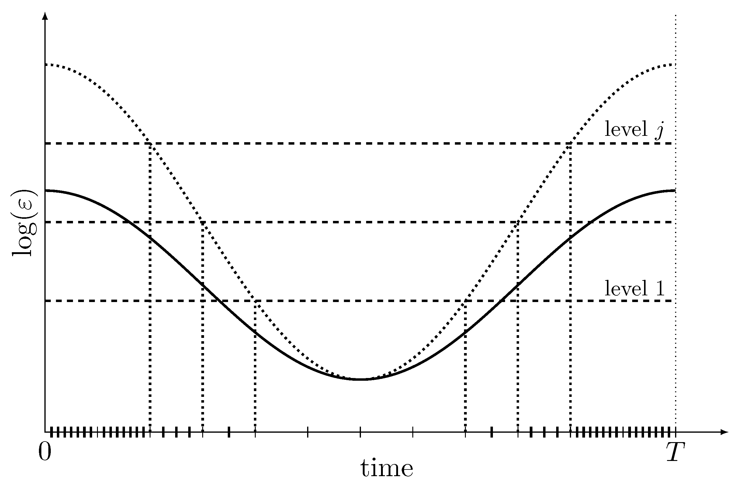
As stated in [16], the multi-level adaptive mesh refinement process starts with discretizing the time interval $[t_0,t_f]$ in a coarse mesh used to solve the NLP problem associated to the OCP in order to catch the main structure of the solution. The subintervals of time where the desired accuracy is not achieved are refined taking into account different levels of refinement in a single iteration, i.e., they are divided into smaller subintervals according to user-defined levels of refinement. This procedure adds more node points to the subintervals in higher levels of refinement, corresponding to higher errors, and it adds less node points to those in lower refinement levels (Figure 4).

In order to proceed with the mesh refinement strategy, we have to define a refinement criterion and a stopping criterion.

As refinement criterion we consider the estimate of the relative error of the adjoint multipliers (dual variables). At each refinement step, the local error of the multipliers $\left({\epsilon }_{\mathbf{q}}\right)$ is evaluated for each time instant t and the procedure selects which time intervals should be further refined:

$${\epsilon }_{\mathbf{q}}\left(t\right)=\left|\left|{\mathbf{q}}_{\mathrm{MP}}\left(t\right)-{\mathbf{q}}_{\mathrm{KKT}}\left(t\right)\right|\right|$$

where ${\mathbf{q}}_{\mathrm{MP}}$ are the multipliers which are solution of the differential equation system given by the maximum principle [20,28], and ${\mathbf{q}}_{\mathrm{KKT}}$ are the multipliers obtained by applying the Kuhn–Tucker conditions to nonlinear optimization problem which results from the transcription of the optimal control. This criterion is chosen because these multipliers give sensitivity information. Furthermore, ${\mathbf{q}}_{\mathrm{MP}}$ are solutions to a linear differential equation system, which can be easily solved in a faster way and with higher accuracy.

For the stopping criterion, we consider a threshold for the relative error of the trajectory. At each refinement iteration, the the $L^{\infty }$ norm of the relative error of the primal variables $\left({\epsilon }_{\mathbf{x}}\right)$ is computed and this information is taken into account when deciding if the refinement procedure should continue. We do not need to compute ${\epsilon }_{\mathbf{x}}\left(t\right)$ for all t—as in the case of the refinement criteria—but just an estimate of ${\left|\left|{\epsilon }_{\mathbf{x}}^{\left(j\right)}\right|\right|}_{\infty }$ which is much faster to obtain.

Since the proposed procedure increases the number of nodes, a greater computational time would be expected. To decrease the CPU time, when going from a coarse mesh to a refined one progressively, the previous solution is used as a warm start for the next iteration. This action proved to be vital in the decreasing of the overall computational time.

This algorithm was developed and tested in [16] for solving a problem with a nonholonomic system and the reported results show that the proposed strategy can solve the problems, spending only 4% of the time required by the standard methods, and therefore can be used in real-time optimization-based control schemes.

The results obtained by applying the AMR procedure to kite power systems are described in the next section.

5. Numerical Results

The proposed algorithm was implemented in MATLAB R2016b combined with the Imperial College London Optimal Control Software—ICLOCS—version 0.1b [29].

We consider the simulation parameters of the kite system defined in

Table 1. Parameters.

Parameter	Value
$\rho$	1.2 kg m−3
$v_w$	10 m s−1
g	9.8 m s−2
m	1 kg
A	10 m2

with the aerodynamic coefficients (adapted from [18]).

$$\left\{\begin{array}{cc}\hfill c_{\mathrm{D}}\left(\alpha \right)& =0.012+0.01\alpha \hfill \\ \hfill c_{\mathrm{L}}\left(\alpha \right)& =0.3+0.1\alpha .\hfill \end{array}\right.$$

5.1. 2D Problem Results

We solve the simpler problem restricted to two dimensions ($\varphi =0$) and we impose that the terminal state should be near the initial one. We consider the state $\mathbf{x}=(r,\beta ,\dot{\beta })$, the control $\mathbf{u}=\left(v_t,\alpha \right)$, the dynamic equation

$$\begin{array}{cc}\hfill \dot{\mathbf{x}}& =\left[\begin{array}{c}{v}_t\\ \dot{\beta }\\ {\displaystyle \frac{1}{mr}}\left(-gmcos\left(\beta \right)+F_{\beta }^{aer}\left(\alpha \right)-2m\dot{r}\dot{\beta }\right)\end{array}\right]:=\mathbf{f}(\mathbf{x},\mathbf{u})\hfill \end{array}$$

and

$$T=-gmsin\left(\beta \right)+F_r^{aer}\left(\alpha \right)+mr{\dot{\beta }}^2.$$

The problem $\left(P_2\right)$ in 2D can be stated as:

$$\begin{array}{cccccc}\hfill \mathrm{Maximize}& \underset{0}{\overset{20}{\int }}{e}^{-t}\dot{r}T\mathrm{d}\mathrm{t}\hfill & & & & \\ \hfill \mathrm{subject}\mathrm{to}& & & & & \\ & \dot{\mathbf{x}}\left(t\right)=\mathbf{f}(\mathbf{x},\mathbf{u})\hfill & & & & \hfill \mathrm{a}.\mathrm{e}.t\in [0,20]\\ & -5\le v_t\le 5\hfill & & & & \hfill \mathrm{a}.\mathrm{e}.t\in [0,20]\\ & -5^{\circ }\le \alpha \left(t\right)\le {10}^{\circ }\hfill & & & & \hfill \mathrm{a}.\mathrm{e}.t\in [0,20]\\ & 10\le r\left(t\right)\le 500\hfill & & & & \hfill \forall t\in [0,20]\\ & {30}^{\circ }\le \beta \left(t\right)\le {120}^{\circ }\hfill & & & & \hfill \forall t\in [0,20]\\ & {\mathbf{x}}_0=\left(10,{80}^{\circ },0\right)\hfill & & & & \\ & \left|\right|{\mathbf{x}}_f-{\mathbf{x}}_0\left|\right|<\epsilon \hfill & & & & \end{array}$$

This problem ($P_2$) is solved with an adaptive mesh refinement strategy [16] with two meshes:

${\pi }_{\mathrm{ML}}$:

The mesh generated by the adaptive refinement strategy

${\pi }_{\mathrm{F}}$:

The equidistant spacing mesh considering the lowest $\Delta t$ of ${\pi }_{\mathrm{ML}}$

The results can be seen in Figure 5 and Figure 6a,b, and the efficiency of the optimal control algorithms is reported in

Table 2. Efficiency comparison for each time-mesh.

${\mathit{\pi }}_{\mathit{j}}$	${\mathit{N}}_{\mathit{j}}$	$\Delta {\mathit{t}}_{\mathit{j}}$	${\mathit{I}}_{\mathit{j}}$	Objective	${\left|\left|{\mathit{\epsilon }}_{\mathit{x}}^{\left(\mathit{j}\right)}\right|\right|}_{\infty }$	CPU Time (s)
						Solve	${\mathit{\epsilon }}_{\mathit{x}}$
${\pi }_0$	51	$\raisebox{1ex}{$1$}\!\left/ \!\raisebox{-1ex}{$50$}\right.$	253	53.216968	1.795 × 10−2	4.754	0.107
${\pi }_1$	474	$\raisebox{1ex}{$1$}\!\left/ \!\raisebox{-1ex}{$500$}\right.$	122	54.156063	2.328 × 10−3	4.722	0.856
${\pi }_2$	2877	$\raisebox{1ex}{$1$}\!\left/ \!\raisebox{-1ex}{$5000$}\right.$	26	54.266839	3.168 × 10−4	6.107	3.383
${\pi }_{\mathrm{ML}}$	2877	$\raisebox{1ex}{$1$}\!\left/ \!\raisebox{-1ex}{$5000$}\right.$	401	54.266839	3.168 × 10−4	15.583	4.346
${\pi }_{\mathrm{F}}$	5001	$\raisebox{1ex}{$1$}\!\left/ \!\raisebox{-1ex}{$5000$}\right.$	1342	54.266873	2.201 × 10−4	431.234	10.913

where we can see that the use of the adaptive mesh refinement strategy reduces the computational time by about 29 times.

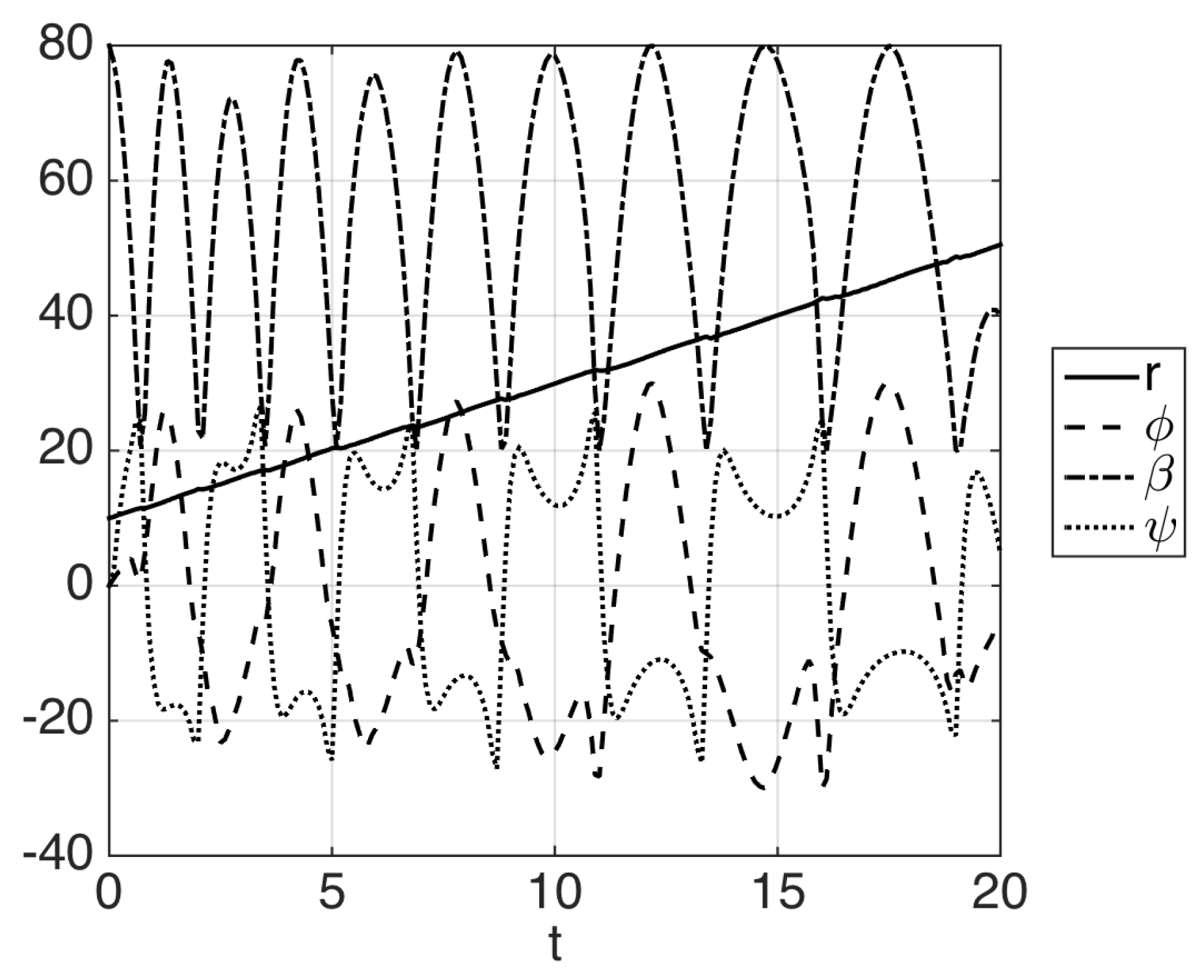
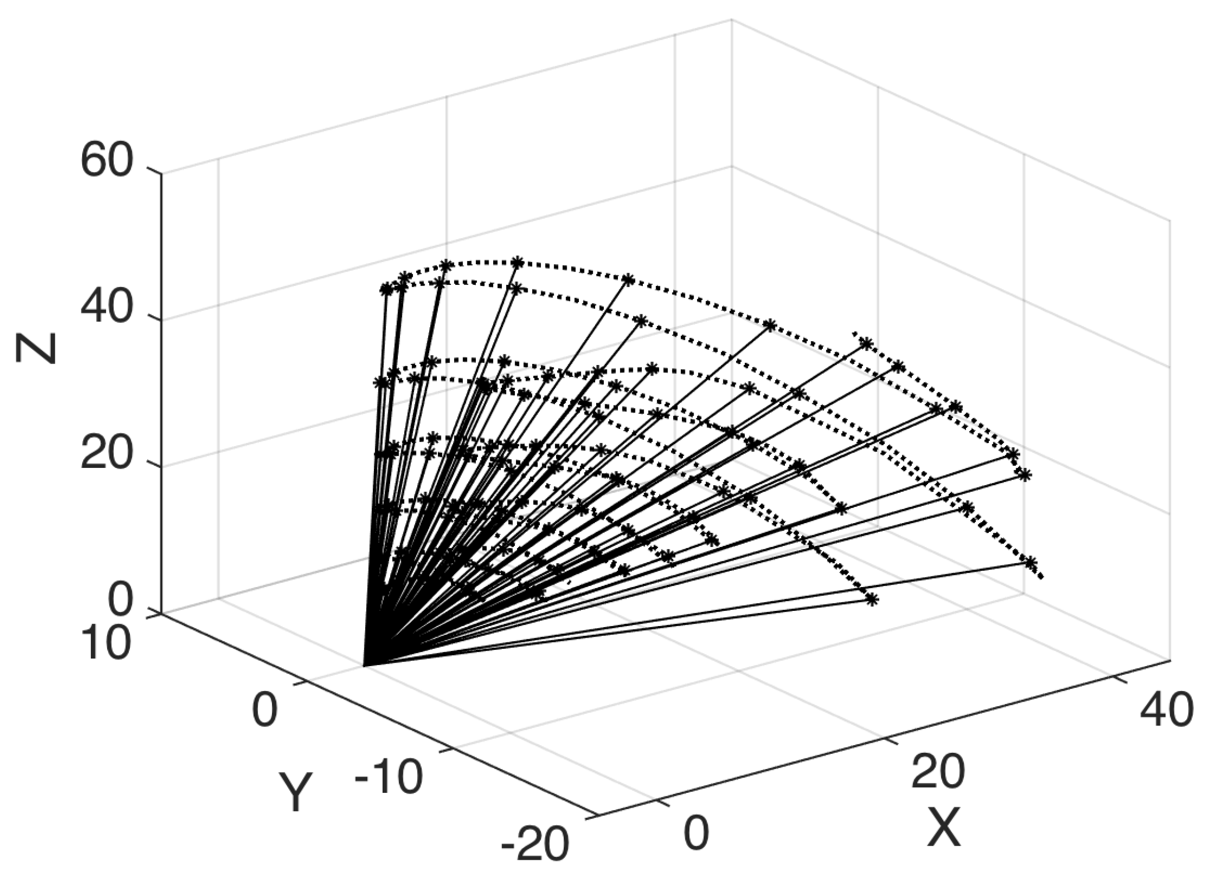
5.2. 3D Problem Results

Considering $t\in [0,20]$, the problem $\left(P_1\right)$ in 3D can be stated as follows:

$$\begin{array}{cc}\hfill \mathrm{Maximize}& \underset{0}{\overset{20}{\int }}\dot{r}T\mathrm{d}\mathrm{t}\hfill \\ \hfill \mathrm{subject}\mathrm{to}\\ & \dot{\mathbf{x}}\left(t\right)=\left[\begin{array}{c}\dot{r}\\ \dot{\varphi }\\ \dot{\beta }\\ a_t\\ {\displaystyle \frac{1}{mrcos\left(\beta \right)}}{\mathrm{F}}_{\varphi }\\ {\displaystyle \frac{1}{mr}}{\mathrm{F}}_{\beta }\end{array}\right]:=\mathbf{f}(\mathbf{x},\mathbf{u})\hfill & \hfill \mathrm{a}.\mathrm{e}.t\in [0,20]\\ & -10\le a_t\left(t\right)\le 10\hfill & \hfill \mathrm{a}.\mathrm{e}.t\in [0,20]\\ & -5^{\circ }\le \alpha \left(t\right)\le {10}^{\circ }\hfill & \hfill \mathrm{a}.\mathrm{e}.t\in [0,20]\\ & -{60}^{\circ }\le \psi \left(t\right)\le {60}^{\circ }\hfill & \hfill \mathrm{a}.\mathrm{e}.t\in [0,20]\\ & \mathbf{x}\left(0\right)={\mathbf{x}}_0=(10,0,{80}^{\circ },3,0,0)\hfill \\ & 10\le r\left(t\right)\le 500\hfill & \hfill \forall t\in [0,20]\\ & -{30}^{\circ }\le \varphi \left(t\right)\le {30}^{\circ }\hfill & \hfill \forall t\in [0,20]\\ & {20}^{\circ }\le \beta \left(t\right)\le {80}^{\circ }\hfill & \hfill \forall t\in [0,20]\end{array}$$

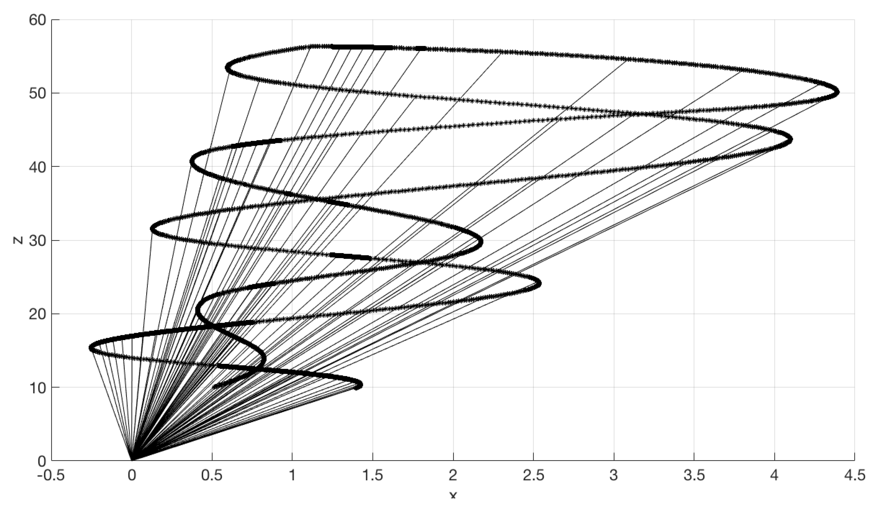
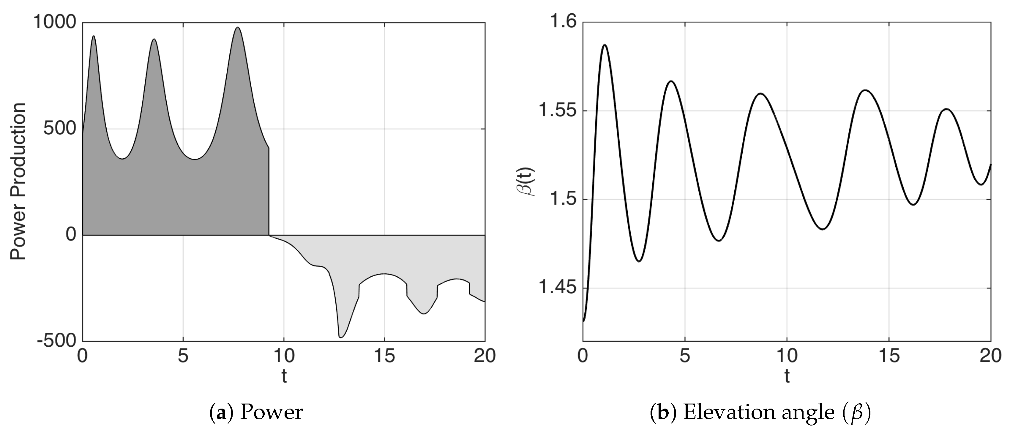
This problem is also solved with the adaptive mesh refinement strategy (AMR). The results can be seen in Figure 7, Figure 8, Figure 9 and Figure 10. We tried to solve the same problem using an equidistant-spaced time-mesh in order to compare the results. However, in such a mesh we could not make the optimizer converge within a reasonable limit for the maximum number of iterations (3000).

6. Conclusions

We address an optimal control problem of generating electricity through kite power systems. The obtained solution comprises the trajectories and controls for the kite that maximize the total energy produced in a given interval. We report results that show that with an adaptive mesh refinement (AMR) strategy the problem can be solved with high level of accuracy and (in simplified versions) much faster. A simplified problem in two dimensions was solved with the AMR 29 times faster than with an equidistant mesh leading to the same level of accuracy.

The complete 3D problem was successfully solved using the AMR strategy, while when using the equidistant mesh leading to the same level of accuracy, the maximum number of iterations of the nonlinear optimization solver was exceeded.

The use of KPSs to generate electrical power at an utility level will require wind farms with multiple kites sharing the same space. A collision avoidance mechanism would then have to be devised. The optimal control formulation is an adequate framework to deal with the trajectory constraints resulting from the collision avoidance restrictions. See [30] for further details.