A Novel Partial Discharge Ultra-High Frequency Signal De-Noising Method Based on a Single-Channel Blind Source Separation Algorithm

Abstract

To effectively de-noise the Gaussian white noise and periodic narrow-band interference in the background noise of partial discharge ultra-high frequency (PD UHF) signals in field tests, a novel de-noising method, based on a single-channel blind source separation algorithm, is proposed. Compared with traditional methods, the proposed method can effectively de-noise the noise interference, and the distortion of the de-noising PD signal is smaller. Firstly, the PD UHF signal is time-frequency analyzed by S-transform to obtain the number of source signals. Then, the single-channel detected PD signal is converted into multi-channel signals by singular value decomposition (SVD), and background noise is separated from multi-channel PD UHF signals by the joint approximate diagonalization of eigen-matrix method. At last, the source PD signal is estimated and recovered by the l₁-norm minimization method. The proposed de-noising method was applied on the simulation test and field test detected signals, and the de-noising performance of the different methods was compared. The simulation and field test results demonstrate the effectiveness and correctness of the proposed method.

1. Introduction

Partial discharge (PD), which is caused by insulation defects, can be utilized to evaluate the insulation state of high voltage devices [1,2,3]. Since ultra-high frequency (UHF) signals (0.3–3 GHZ) will be also produced and propagated outside through the non-metal shielding dielectrics when PD occurs, the UHF antenna sensor can be used to detect the PD of high-voltage (HV) apparatus [4]. However, since the PD UHF signal amplitudes are very low in the early insulation defects, and vulnerable to interference due to the numerous external electromagnetic waves, the detected PD signal will have serious waveform distortion, even submerged in background noise interference. Thus, the de-noising method has attracted extensive attention from researchers.

Periodic narrow-band interference and Gaussian white noise are the main components of background noise interference. Digital PD de-noising methods have been widely used, with the advantage of good noise suppression performance. There are several digital PD de-noising technologies, such as Fast Fourier transform (FFT) thresholding filtering, adaptive digital filtering (AF), empirical mode decomposition (EMD), undecimated Wavelet Transform (UWT), and adaptive wavelet thresholding (AWT) methods. Although FFT thresholding filtering and the AF method can effectively suppress the periodic narrow-band interference, the signal will be distorted when the frequency of PD signal and narrow-band interference are coincident [5,6]. The EMD method contains the modal aliasing problem which affects the de-noising performance [7]. The UWT method is a commonly used wavelet de-noising method to suppress the noise interference [8]. The AWT method can effectively suppress Gaussian white noise; however, since the wavelet basis and decomposed layers are difficult to select, the de-noising PD signal will be distorted when the wavelet transform method is used to suppress the periodic narrow-band interference [9].

A chaotic oscillator method was proposed to effectively suppress the narrow-band interference signal [10], but it cannot setup the system periodic frequency, and the calculation quantity is large. A reverse separation method, based on the independent component analysis (RS) method, was proposed to reversely separate the partial charge signal from the noise interference signals [11], but the de-noising PD signal amplitude was changed. A sparse representation de-noising method was proposed in [12], but it needs to establish the atomic library and takes a long time to complete the iteration calculation. A generalized S-transform module time-frequency matrix method (GSMT) was proposed for de-noising the PD signals in [13], but it could not effectively suppress the amplitude modulated narrow-band interference during wireless communication, and large amounts of matrix operations were needed. To suppress the Gaussian white noise, a mathematical morphology filters (MMF) method was proposed to suppress the Gaussian white noise in [14], and a novel singular value decomposition (SVD) method was proposed to suppress the Gaussian white noise and the original PD signal could be more accurately recovered in [15].

Blind source separation technology (BSS) has been proposed to effectively separate the source signals when the characteristic parameters and models of source signals are unknown [16,17,18]. All noise interference signals and original PD signals can be seen as the source signals, and the detected PD UHF signals are considered to be the observation signals. Hence, the original PD signal can be separated from the observation signals without solving the time-frequency information of narrow-band interference signals in the PD UHF signals.

This paper proposed a novel PD UHF de-noising method based on a single-channel blind source separation algorithm (BSS), which can effectively suppress the background noise interference of PD UHF signals and reduce the distortion of de-noising PD UHF signals. Firstly, the principle of de-noising method based on BSS is introduced in Section 2. The single-channel signal can be converted into multi-channel signals by the singular value decomposition (SVD), and background noise is separated from multi-channel PD UHF signals by the joint approximate diagonalization of eigen-matrices, and the PD UHF signal from which the noise has been separated from can be recovered by estimation of the l₁-norm minimization method. The proposed method is applied in the simulation test and field test detected PD UHF signals in Section 3 and Section 4. In addition, the de-noising performances of different de-noising methods were evaluated and compared. The experimental results verify the effectiveness and correctness of the proposed method. In addition, conclusions are summarized in Section 5.

2. Single-Channel Blind Source Separation De-Noising Algorithm

2.1. BSS Mathematical Model

Assume s(t) = [s₁(t), s₂(t), …, s_N(t)] is the unknown independent vector from N signal sources, x(t) = [x₁(t), x₂(t), …, x_M(t)] is the known vector detected by M sensors after several transmission process mixtures and t is the time series. Since the superposition of the PD signal, periodic narrow-band interference signal and Gaussian white noise signal in the PD UHF signal is linear mixed, the mathematical model of linear mixed BSS can be expressed as [19,20].

$$\mathit{x}(t)=\mathit{A}\mathit{s}(t)$$

(1)

where A is the mixed matrix with M in N order.

Then, the unknown signal vector s(t) can be separated from the detected signal, x(t), by solving the separation matrix, W. Assume y(t) = [y₁(t), y₂(t), …, y_N(t)] is the output signal vector after BSS. The mathematical model of BSS is

$$\mathit{y}(t)=\mathit{W}\mathit{x}(t)=\mathit{W}\mathit{A}\mathit{s}(t)$$

(2)

where W is the separation matrix with N in M order.

When M ≥ N, it is non-underdetermined blind source separation. The unknown PD signal vector s(t) can be directly solved by Equation (2). When M < N, it is underdetermined blind source separation. Since the solution of Equation (2) is not unique, the optimal estimate solution of s(t) can be only calculated by the estimation method. However, for PD UHF de-noising, a single sensor is always used to detect the PD UHF signal (M = 1), and the number of source signals (N) (includes the PD signal, white Gaussian noise signal and other narrow-band interference signals) will be larger than three (N ≥ 3), which is called single-channel BSS. Hence, the BSS based on matrix computation is not feasible. The one-dimensional signal vector, x(t), detected by single channel should be decomposed into multiple time-domain signals. The single-channel PD signals can be converted into multiple-channel signals, through establishing the virtual channels, meeting the requirements of non-underdetermined blind source separation.

2.2. Number Estimation of Source Signals

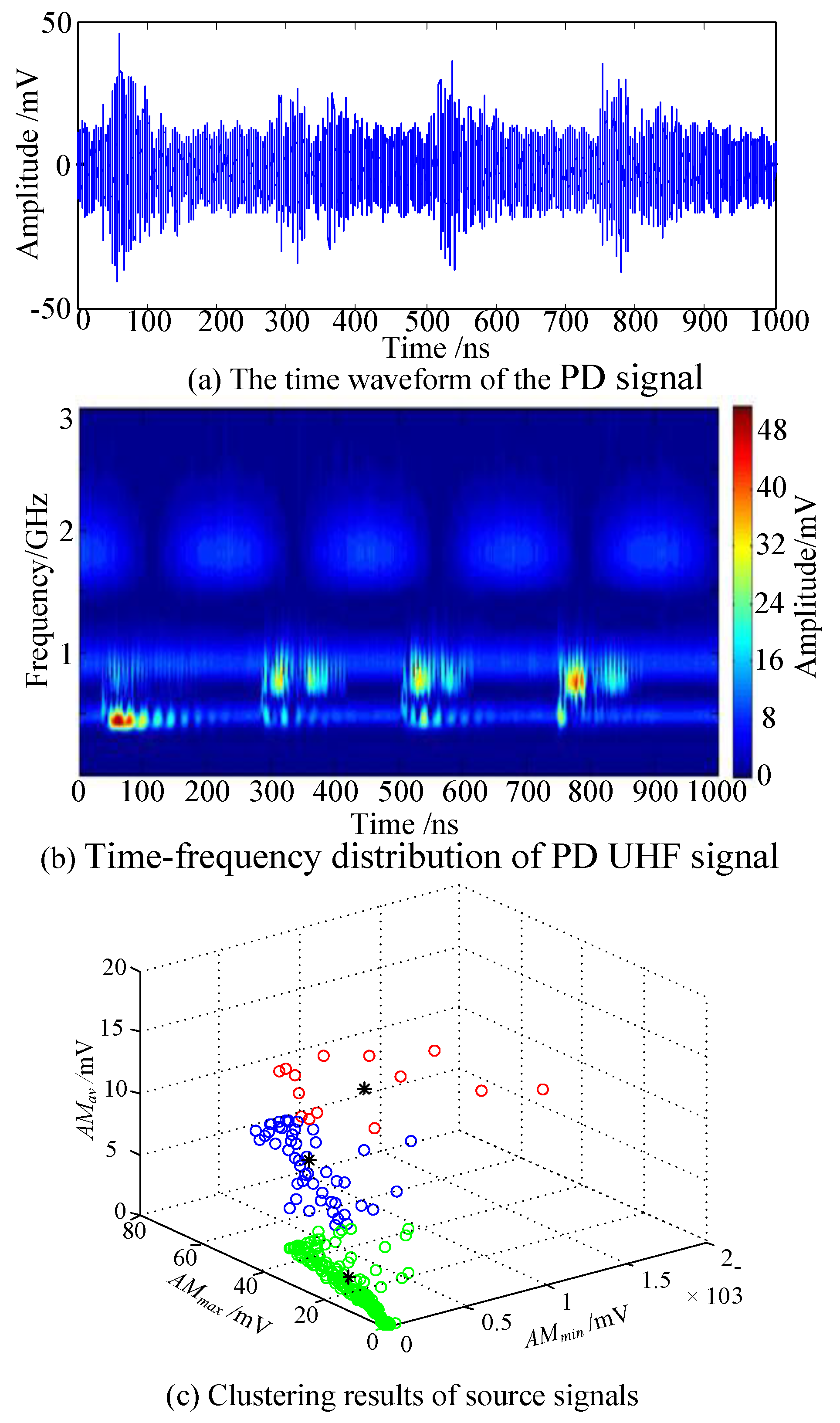
To establish the virtual channels, the number of source signals (N) is needed. Firstly, the one-dimensional time domain signal is mapped to a two-dimensional time-frequency domain through the time-frequency analysis of detected source signals. The amplitude–time source signals can be converted into amplitude–time–frequency signal. Hence, the number of source signals (N) can be obtained.

Due to the advantages of flexibility of time–frequency resolution and convenience, S-transform is used to convert the source signals. S-transform function can be expressed as [21]

$$\mathit{s}(\tau ,f)={\displaystyle \underset{-\infty }{\overset{\infty }{\int }}\mathit{x}(t)\mathit{g}(t-\tau ,f)}{e}^{-j2\pi ft}dt={\displaystyle \underset{-\infty }{\overset{\infty }{\int }}\mathit{x}(t)}\frac{f}{\sqrt{2\pi }}{e}^{-\frac{f^2{(t-\tau )}^2}{2}}{e}^{-j2\pi ft}dt$$

(3)

where f represents the frequency, t and τ represent the time, and g(t − τ, f) represents the Gaussian window function.

Since the frequency distribution of periodic narrow-band interference is concentrated and the amplitude is large, a clustering analysis method of frequency section characteristic parameters, based on the time–frequency matrix of S-transform, is proposed to estimate the number of signal sources. The proposed clustering analysis method is as follows:

Step 1: Solve the time–frequency matrix based on S-transform, the frequency sections are extracted at each 10 MHz interval, such as 0~10 MHz, 10 MHz~20 MHz, etc.

Step 2: Compare the amplitudes of all time–frequency sampling points for each frequency section. The maximum amplitude (AM_max) is characteristic parameter 1, and the minimum amplitude (AM_min) is characteristic parameter 2.

Step 3: Solve the average amplitude (AM_av) for all time–frequency sampling points for each frequency section as characteristic parameter 3.

Step 4: According to the characteristic parameters extracted in Step 2 and Step 3, the fast search and find of the density peaks clustering (FSFDPC) algorithm is proposed to cluster [22]. The cluster number, which is the amount of periodic narrow-band interference (N_pn), can be obtained. The FSFDPC algorithm has better convergence capacities.

Step 5: According to the source signal statistical characteristics of blind source separation, the number of PD UHF signals and the Gaussian white noise signal are equal to 1. Hence, the number of the source signals is N = N_pn + 2.

2.3. Multi-Channel Detected Signal Recombination

For single-channel BSS, the traditional method of constructing virtual channels is the empirical mode decomposition (EMD), which can decompose the single-channel signal into intrinsic mode function signals. However, since the PD UHF signal and periodic narrow-band interference source signal are independent, the traditional method has the modal aliasing problem which will negatively affect the final signal separation result. Therefore, this paper proposed a novel multi-channel detected signal recombination method based on SVD. The trajectory matrix (X) of detection signal x(t) can be expressed as [23,24]

$$\mathit{X}=\mathit{U}{\mathit{\Lambda }}_a{\mathit{V}}^T$$

(4)

where X is the trajectory matrix, U and V are the orthogonal matrices with m by n order, respectively, Λ_a = diag (a₁, a₂, …, a_n) is a diagonal matrix, a₁, a₂, …, a_n are the singular values of mixed matrix A.

Since matrix A with rank k can be expressed as the sum of k submatrices with rank 1,

$$\mathit{X}=\mathit{U}{\mathit{\Lambda }}_a{\mathit{V}}^T={\displaystyle \sum _{i=1}^k{a}_i{u}_i{v}_i^T=}{\displaystyle \sum _{i=1}^k{a}_i{\mathit{X}}_i}$$

(5)

where u_i and v_i are the singular value vectors of the i-th column of matrices U and V, respectively. X_i is a submatrix.

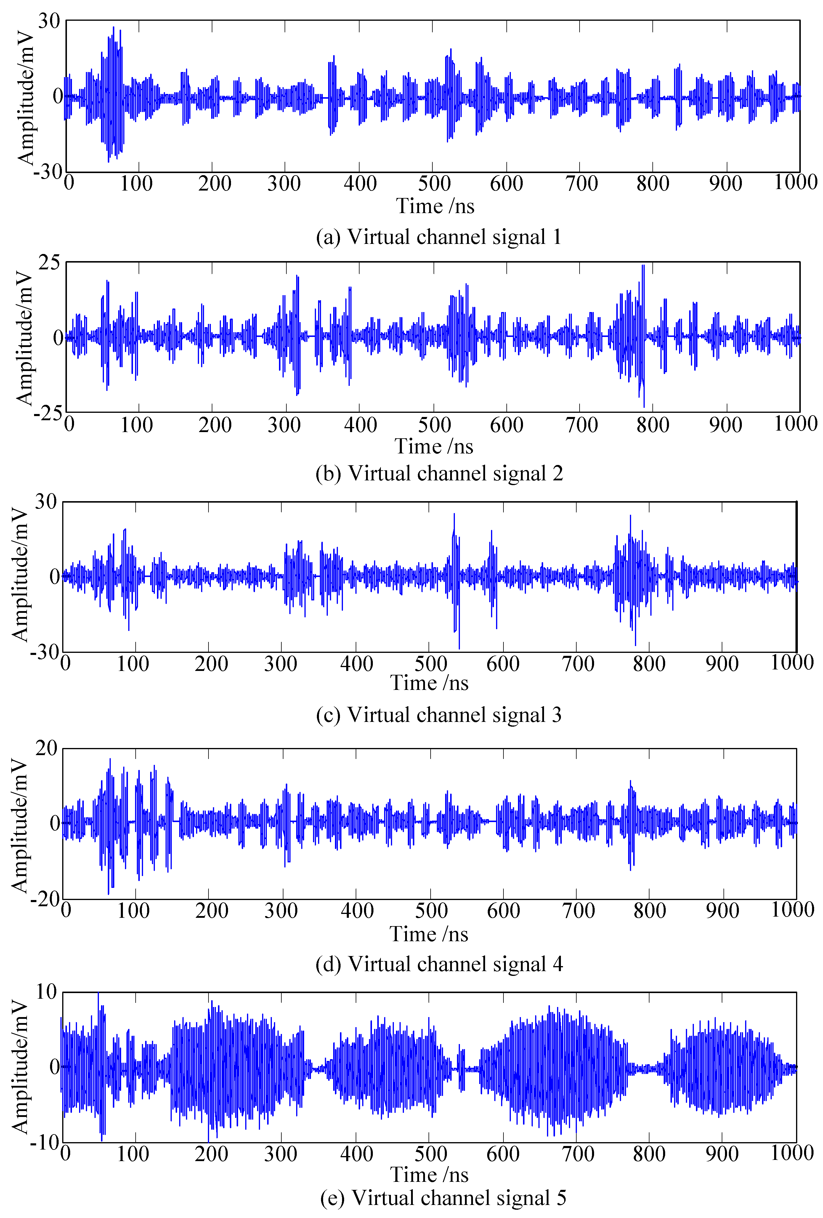
Each submatrix in SVD is multiplied by the singular value weight and two eigenvectors are derived from matrices U and V, respectively. The submatrix and the singular value (a_i) have a positive correlation. Hence, since the time–frequency distribution of the PD signal and periodic $narrow-band$ interference is relatively concentrated, the amount of information of the singular values is large. When the time–frequency distribution of Gaussian white noise signal is dispersed, the amount of information of the singular values is smaller. In addition, the submatrices for different singular values (a_i) are statistically independent, the corresponding submatrices with the first N singular values can be obtained through the SVD calculation of the single-channel detection signal, x(t). Then, the virtual channels are constructed by signal reconstruction calculation, and the multi-channel signals can be recombined for blind source separation de-noising.

Hence, the proposed multi-channel detected signal recombination method is as follows:

Step 1: Construct a trajectory matrix (X) of signal x(t), as follows:

$$\mathit{X}=\left[\begin{array}{cccc}{x}_1& x_2& \dots & x_n\\ x_2& x_3& \dots & x_{n+1}\\ ⋮& ⋮& & ⋮\\ x_m& x_{m+1}& \dots & x_{n+m-1}\end{array}\right]$$

(6)

Step 2: The SVD calculation for trajectory matrix X, and the singular value sequence a₁, a₂, …, a_N is obtained.

Step 3: Extract the first N singular value sequence (a₁, a₂, …, a_N) and the corresponding submatrices. Reconstruct the virtual channels.

$${\mathit{X}}_j=\mathit{U}{\mathit{\Lambda }}_j{\mathit{V}}^T=a_j{u}_j{v}_j^T$$

(7)

where C_j is the virtual channel signal trajectory matrix. Λ_j = diag ((0, …, 0), a_N, (0, …, 0)), j = 1, 2, …, N.

Step 4: Inversely calculate the trajectory matrix (C_j), according to Step 1. The virtual channel signal, C_j(t), can be obtained.

Step 5: Recombine the virtual channel signal, C_j(t), and the original single-channel detected signal, x(t), as the novel multi-channel detected signal, D(t) = [x(t), C₁(t), C₂(t), …, C_N(t)]. It will become the non-underdetermined blind source separation.

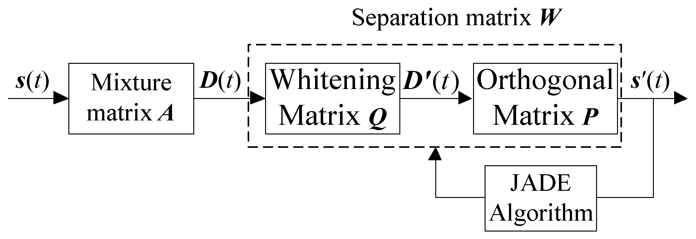
2.4. BSS De-Noising Method Based on the JADE Algorithm

The separation matrix (W) is the most important for BSS. This paper proposed the JADE algorithm to solve the separation matrix, W. The JADE algorithm introduces a fourth-order cumulant of multivariate data to estimate separation matrix W by characteristics decomposition and joint approximation diagonalization [25]. The blind source separation de-noising method based on the JADE algorithm can be divided into two steps to solve the separation matrix (W) whitening process and orthogonal transform processes, as shown in Figure 1.

Firstly, the multi-channel detected signal, D(t), should be whitening processed to eliminate the second-order correlation between the components. The whitening process can be expressed as [25]

$${\mathit{D}}^{\prime }(t)=\mathit{Q}\mathit{D}(t)=\mathit{Q}\mathit{A}\mathit{s}(t)=\mathit{C}\mathit{s}(t)$$

(8)

where Q is the whitening matrix, D′(t) is the signal after the whitening process, in which each component is relatively independent and the variance is 1, and matrix C is the product of matrices Q and A.

Assume R_x is the correlation matrix of the multi-channel detection signal D(t), and D(t) can be eigenvalue decomposed as

$${\mathit{R}}_x=\mathit{E}{{\mathit{\Lambda }}_{\lambda }}^2{\mathit{E}}^T$$

(9)

where matrix ${{\mathit{\Lambda }}_{\lambda }}^2=\mathrm{diag}({\lambda }_1^2,{\lambda }_2^2,\dots ,{\lambda }_n^2)$ is the orthogonal matrix, in which the diagonal elements are the eigenvalues of matrix R_x, and the corresponding standard orthonormal eigenvector is the column vector of characteristic matrix E.

The whitening matrix (Q) can be expressed as

$$\mathit{Q}={{\mathit{\Lambda }}_{\lambda }}^{-1/2}{\mathit{E}}^T$$

(10)

Since the component variances of s(t) and D′(t) are both 1, each element of s(t) is independent, and each element of D(t) is orthogonal; matrix C is an orthogonal normalized matrix and can be expressed as

$$\mathit{C}{\mathit{C}}^T={\mathit{C}}^T\mathit{C}={\mathit{I}}_N$$

(11)

where I_N is the N-order unit matrix.

The matrix, D′(t), after the whitening process needs the orthogonal transformation to make aure that the components after blind source separation are not correlated and the variance is 1. The orthogonal transformation process can be expressed as

$${\mathit{s}}^{\prime }(t)=\mathit{P}{\mathit{x}}^{\prime }(t)$$

(12)

where matrix P is the orthogonal matrix, s′(t) is the approximate s(t) by orthogonal transformation estimation.

The fourth-order cumulant of D′(t) is

$$cum(x_i^{\prime },x_j^{\prime },x_h^{\prime },x_l^{\prime })={\displaystyle \sum _{p=1}^L{k}_p{c}_{ip}}{c}_{jp}{c}_{hp}{c}_{lp}$$

(13)

where 1 < i, j, h, l < L, k_p is the fourth-order cumulant of each element and c_ip, c_jp, c_hp, c_lp are the elements of (i, p), (j, p), (h, p), (l, p) of matrix C, respectively.

For any matrix (M) with L by L order, the fourth-order cumulant matrix, Q_D(M), can be expressed as

$${[{\mathit{Q}}_D(\mathit{M})]}_{ij}={\displaystyle \sum _{h=1}^L{\displaystyle \sum _{l=1}^{L}cum(x_i,x_j,x_h,x_l)m_{hl}}}$$

(14)

where m_hl is the element (h, l) of matrix M.

According to Equation (9), Equation (14) is

$${\mathit{Q}}_D(\mathit{M})=\mathit{P}{\mathit{Q}}_S(\mathit{M}){\mathit{P}}^T$$

(15)

where Q_S(M) is the fourth-order cumulant matrix of s(t).

Since the components of s(t) are statistically independent, matrix Q_S(M) is the diagonal matrix. Select a matrix, M = [M₁, M₂, …, M_r], the orthogonal matrix (P) can be solved by joint approximate diagonalization of matrix Q_D(M). The quadratic sum of diagonal elements is defined as the evaluation index of the joint approximate diagonalization calculation,

$$\mathit{E}(\mathit{P})={{\displaystyle \sum _{r=1}^L\left|diag(\mathit{P}{\mathit{Q}}_S({\mathit{M}}_r){\mathit{P}}^T)\right|}}^2$$

(16)

The orthogonal matrix P can be solved by minimizing E(P). Then, the whitening matrix (Q) and the separation matrix (W = QP) can be obtained.

2.5. PD Signal Recovery After De-Noising

Since the signal, s′(t), after blind source separation, based on the JADE algorithm, is an approximate signal vector of s(t), the amplitude of s′(t) is different from the source signal. To improve the accuracy of blind source separation, this paper proposed an l₁-norm minimization method to recover the original approximate PD UHF signal, s′(t). For a matrix with M′ by N′ order, ${\mathit{C}}_{N^{\prime }}^{M^{\prime }}$ solutions can be obtained in the l₁-norm minimization [26]. Hence, the minimum norm solution can be obtained through comparison with the solutions. The l₁-norm minimization method is shown as follows:

Step 1: Calculate the ${\mathit{C}}_{N^{\prime }}^{M^{\prime }}$ submatrices with M′ by N′ order of mixture matrix A, which is denoted as B_g = [B_g1, B_g2, …, B_gM′], g = 1, 2, …, ${\mathit{C}}_{N^{\prime }}^{M^{\prime }}$; g₁, …, g_M′ ∈ {1, …, N′}.

Step 2: Solve the minimum l₁-norm solution at t = t₀. The solution can be expressed as

$${\mathit{s}}^{{}^{\prime }(g)}(t_0)=[{\mathit{s}}_{g_1}^{{}^{\prime }(g)}(t_0),\dots ,{\mathit{s}}_{g_{M^{\prime }}}^{{}^{\prime }(g)}(t_0)]={\mathit{B}}^{-1}\mathit{x}(t_0)$$

(17)

Step 3: Calculate the l₁-norm J_g of solution s′^(g)(t₀), as follows

$${\mathit{J}}_g={\displaystyle \sum _b^{N^{\prime }}\left|{\mathit{s}}^{{}^{\prime }(g)}(t_0)\right|},b=1,\dots N^{\prime }$$

(18)

Step 4: Calculate the minimum norm as the approximate signal s′(t₀) at t = t₀ as follows

$${\mathit{s}}^{\prime }(t_0)={\mathit{s}}_{\min }^{\prime }(t_0)=\underset{{\mathit{s}}^{{}^{\prime }(g)}(t_0)}{\min }{\mathit{J}}_g$$

(19)

Step 5: Calculate s′(t) at all time points, reconstruct the PD source signal, and the signal recovery of PD signal is complete.

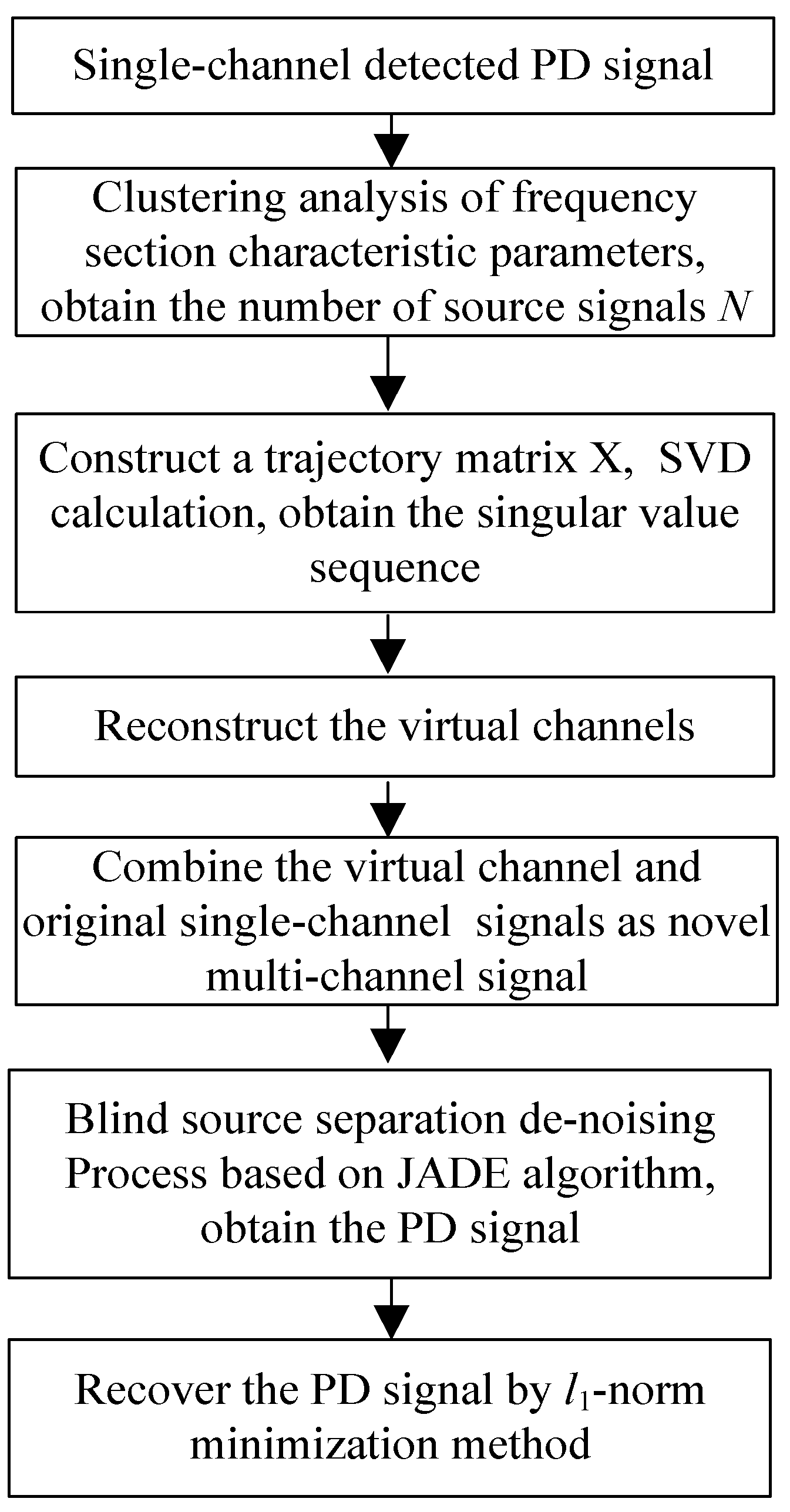
The proposed flow chart for the proposed PD UHF signal de-noising method based on single-channel blind source separation is shown in Figure 2. Firstly, the single-channel detected signal is analyzed through time–frequency analysis by S-transform, the frequency section characteristic parameters based on the time–frequency matrix of S-transform is used for clustering analysis, and the number of source signals (N) can be obtained. Then, construct the trajectory matrix of the detected signal, and the singular value sequence of the corresponding submatrices can be obtained by SVD calculation. The virtual channel can be reconstructed, and novel multi-channel signals can be obtained by combining the virtual channel and original single-channel signals. In addition, the PD signal can be separated from the mixed signals by BSS based on the JADE algorithm. Finally, the PD signal can be recovered by the l₁-norm minimization method.

3. Simulation Test of De-Noising

3.1. Simulation Test Signals

Different types of typical insulation defects are simulated in the gas insulated switchgear (GIS) laboratory test platform, respectively. The corresponding PD UHF signals can be detected by the step voltage test. Firstly, the background noise interference was measured when the PD signals did not generate in GIS. Then, gradually increase the voltage until the remarkably stable PD UHF signals can be detected, the PD signals are recorded.

Table 1. Insulation defects and test voltages.

Insulation Defect Types	Test Voltage	Pulse Sequence
Metal tip	27.8 kV	Pulse 1
Internal air gap	21.6 kV	Pulse 2
Floating potential	22.4 kV	Pulse 3
Free metal particles	29.5 kV	Pulse 4

shows the insulation defects and test voltages. The simulation method for each insulation defect is shown in Figure 3. The simulation test platform and schematic diagram of the simulation test are shown in Figure 4 and Figure 5, where T1 is the voltage regulator, T2 is the PD test transformer (YDTW-25/100, Wuhan Retop Power Equipment Company, Wuhan, China), R1 = 1 MΩ is the protection resistance, R2 = 50 Ω, C1/C2 is the power–frequency voltage divider (TAWF-1000/600), the PD UHF antenna is the Diagnostic Monitoring Systems (DMS) PD UHF antenna sensor (working bandwidth: 0.5~3 GHZ, highest antenna gain: 2.7 dBi, DMS, Glasgow, UK), the oscilloscope which is used to detect the PD UHF signals is WavePro 640Zi (maximum sampling frequency: 20 Gs/s, maximum bandwidth: 4 GHZ, Teledyne LeCroy, Chestnut ridge, New York, NY, USA. ), and N₂/SF₆ mixed gas is filled in GIS (volume ratio of N₂/SF₆: 1:4, 0.5 MPa).

The PD UHF pulse signals produced in four kinds of insulation defects are combined, as shown in Figure 6a. The Gaussian white noise and periodic narrow-band interference should be added into the PD UHF pulse signals. Since the periodic narrow-band interference mainly consists of the carrier communication and mobile phone signals, which are the sine wave signals, with frequencies of 470, 900, and 1800 MHZ. The mathematical models of signals can be expressed as

$$\{\begin{array}{c}{Z}_1(t)=0.005\sin (2\pi \cdot 470\times {10}^6\cdot t)\\ Z_2(t)=0.005\sin (2\pi \cdot 900\times {10}^6\cdot t)\\ Z_3(t)=0.005\sin (2\pi \cdot 1800\times {10}^6\cdot t)\cdot \cos (2\pi \cdot 2\times {10}^5\cdot t)\end{array}$$

(20)

Since the signals of wireless communication are always from the amplitude modulation type, Z₃(t) is the amplitude modulation sine wave model. In addition, the PD signal detection will be interfered by Gaussian white noise; thus, Gaussian white noise with distribution (0, 0.4) is added. Figure 6b shows the final noisy PD signal. It can be seen that the signal is seriously disturbed, and time–domain characteristics of signals cannot be identified.

3.2. De-Noising Results and Discussion

The proposed single-channel blind source separation algorithm was used to de-noise the noisy PD UHF signal in Figure 6b. Four traditional methods were also used for de-noising for comparison, as shown in

Table 2. De-noising method.

Method	De-Noising Method
Method 1	Proposed single-channel blind source separation (BSS)
Method 2	Adaptive filtering de-noising (AF)
Method 3	Adaptive wavelet thresholding de-noising (AWT)
Method 4	Reverse separation based on independent component analysis (RS)
Method 5	Generalized S-transform module time-frequency matrix method (GSMT)
Method 6	Undecimated wavelet transform de-noising method (UWT)

. For the AF algorithm, the least mean square (LMS) adaptive filter algorithm is used. The order of the filter is 255, the transition width of the filter is 100 MHZ, and the minimum width of a stop band is 50 MHZ [27]. For the AWT algorithm, the db10 wavelet is selected as the wavelet basis, and the decomposition layer is 10 [9]. For the RS algorithm, the constructed Hankel matrix is 15,000 by order 5001, and the larger number of singular values is 18 [11]. For the GSMT algorithm, the adjusted parameter of the generalized S-transform is 0.3, and the number of effective singular values is 4 [13].

Firstly, S-transform is used for the time-–frequency analysis of the signal, the time waveform of the signal is shown in Figure 7a, and the time–frequency distribution is shown in Figure 7b. Then the clustering analysis method of frequency section characteristic parameters is used to analysize the time–frequency distribution and estimate the number of source signal; the clustering results are shown in Figure 7c, the number of source signals is N = 5.

The reconstructed virtual channel signals by SVD calculation and trajectory matrix reconstitution are shown in Figure 8. Then, the de-noising PD signal was obtained by the blind source separation de-noising process based on the JADE algorithm and the l₁-norm minimization method, as shown in Figure 9. In addition, four traditional methods in Table 2 were performed for de-noising the PD UHF signals. The de-noising results are shown in Figure 10.

Four evaluation indices are introduced to evaluate the PD UHF signal de-noising performance for each method: signal to noise ratio, root-mean-square error, waveform similarity coefficient, and variation trend parameter. Since the noise interference of the PD UHF signal in Figure 6 is very small, it can be approximately seen as the ideal non-noise original PD signal. A higher signal to noise ratio leads to a greater ability of the de-noising method to suppress interference. The root-mean-square error can show the difference between the de-noising PD and original PD signals. A lower value leads to a smaller distortion of the de-noising PD signal. When the waveform similarity coefficient is closer to 1, the de-noising PD and original PD signals are more similar. The variation trend parameter reflects the variation trend similarity between the de-noising PD and original PD signals. The variation trends for both signals are consistent when the value is closer to 1.

The evaluation results of various methods which were evaluated by the proposed indices are shown in

Table 3. De-noising performance evaluation results.

Evaluation Index	De-Nosing Method	Pulse 1	Pulse 2	Pulse 3	Pulse 4	Pulse 5
Signal to noise ratio	Proposed BSS	18.421	19.322	17.643	17.119	18.064
	AF	2.662	4.723	3.982	5.298	4.209
	AWT	3.816	3.210	2.978	3.382	3.283
	RS	13.982	13.298	13.132	13.309	13.325
	GSMT	11.120	10.872	10.987	10.876	10.897
	UWT	8.142	7.973	8.023	8.487	8.201
Root-mean-square error	Proposed BSS	0.002	0.003	0.003	0.003	0.003
	AF	0.063	0.048	0.023	0.021	0.036
	AWT	0.052	0.059	0.064	0.053	0.055
	RS	0.003	0.003	0.004	0.003	0.003
	GSMT	0.006	0.005	0.006	0.006	0.006
	UWT	0.018	0.021	0.019	0.022	0.020
Waveform similarity coefficient	Proposed BSS	0.988	0.969	0.983	0.911	0.973
	AF	0.343	0.571	0.445	0.625	0.530
	AWT	0.643	0.634	0.667	0.671	0.628
	RS	0.962	0.953	0.968	0.973	0.974
	GSMT	0.893	0.881	0.896	0.878	0.856
	UWT	0.711	0.732	0.740	0.728	0.724
Variation trend parameter	Proposed BSS	1.032	1.048	1.092	1.021	1.051
	AF	1.790	1.532	1.691	1.598	1.614
	AWT	0.616	0.547	0.774	0.694	0.683
	RS	1.070	1.086	1.072	1.086	1.071
	GSMT	1.158	1.171	1.168	1.170	1.15
	UWT	0.863	0.927	0.881	0.893	0.894

.

It can be seen that the proposed de-noising method based on single-channel blind source separation can effectively suppress various noise interference without calculating the characteristic parameters of narrow-band interference, and the distortion of the de-noising PD signal is very small through the recovery method based on l₁-norm minimization method, compared with traditional methods. For Method 2 (AF method), since the frequency of the PD UHF signal and periodic narrow-band interference signal overlap, part of the characteristic quantity of the PD signal will be removed in Method 2, leading to a large distortion of PD signals. This demonstrates that the proposed method has a good performance in suppressing the periodic narrow-band interference signal. For Method 3 (WT method), since the PD UHF signal is complicated and appropriate wavelet basis function is difficult to select, the distortion of the de-noising PD signals is apparent. In addition, the difference between the de-noising and original PD signals is larger in Method 4 (RS method), due to the unknown original PD signal. This demonstrates that, compared with the RS method, the amplitude of the de-noising PD UHF signal can be recovered by the proposed l₁-norm minimization method. For Method 5 (GSMT method), since there is amplitude modulation sine wave periodic narrow-band interference, the submatrix modulus value method cannot be used to suppress the narrow-band interference, the suppression performance for periodic narrow-band interference is not good. Compared with the GSMT method, the proposed method can also effectively suppress the amplitude-modulation narrow-band interference. For Method 6 (UWT method), since the frequency distribution of the periodic narrow-band interference and PD UHF signals overlap, the suppressing performance is not good.

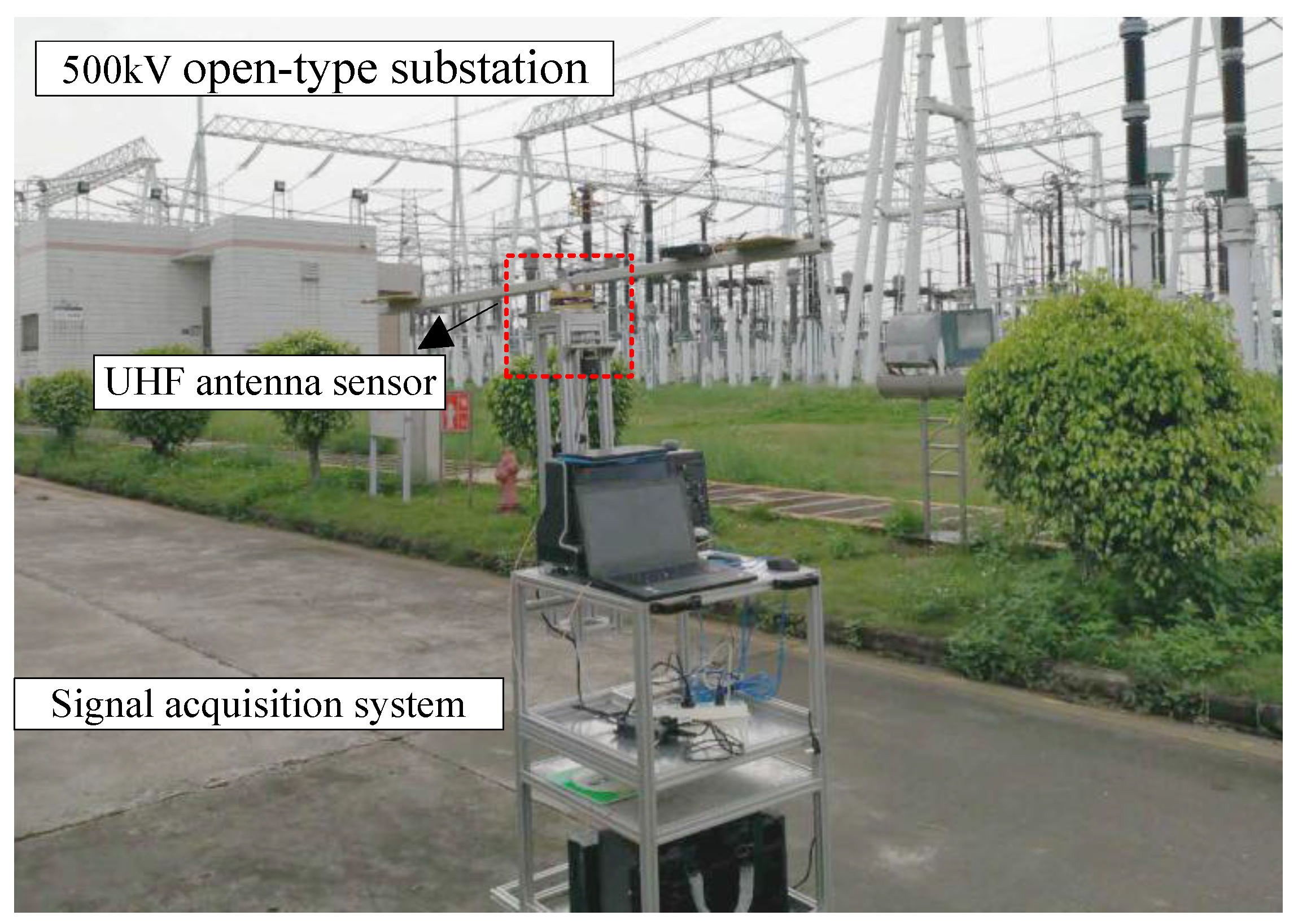
4. Field Test for De-Noising

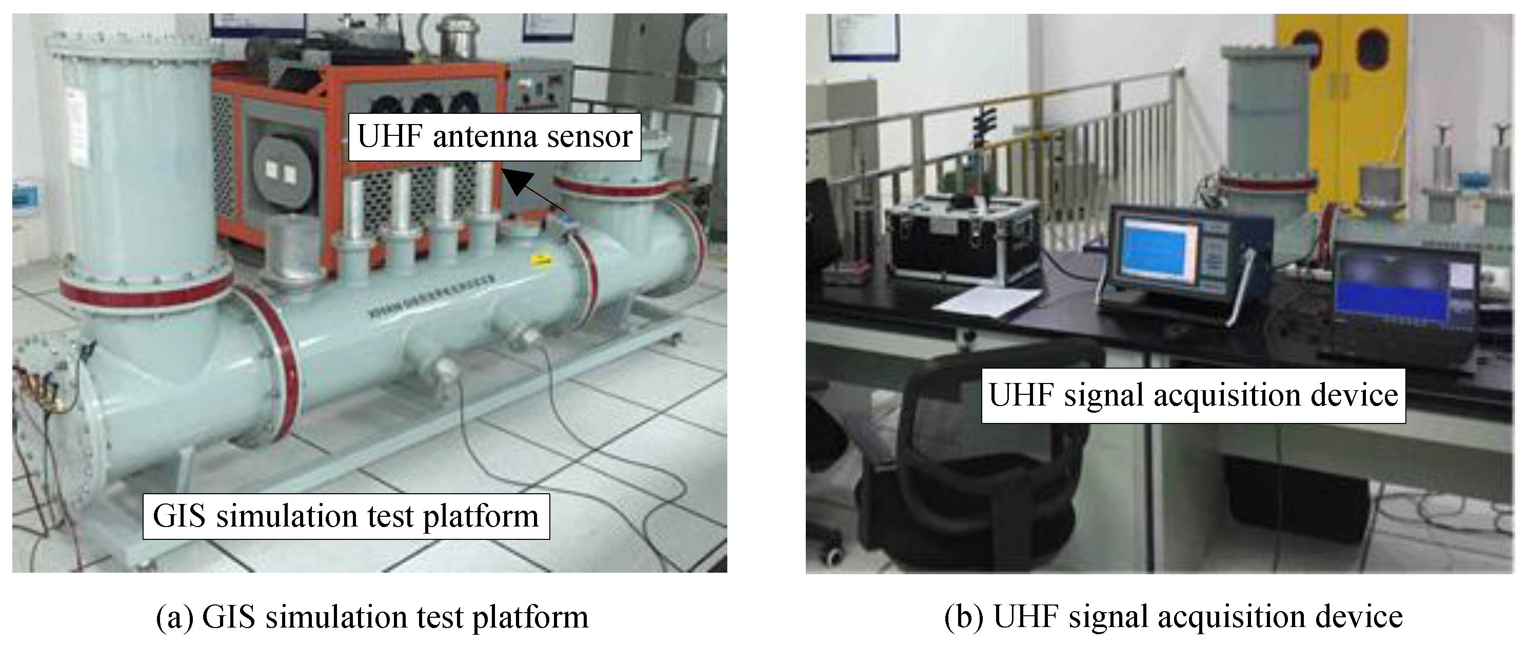
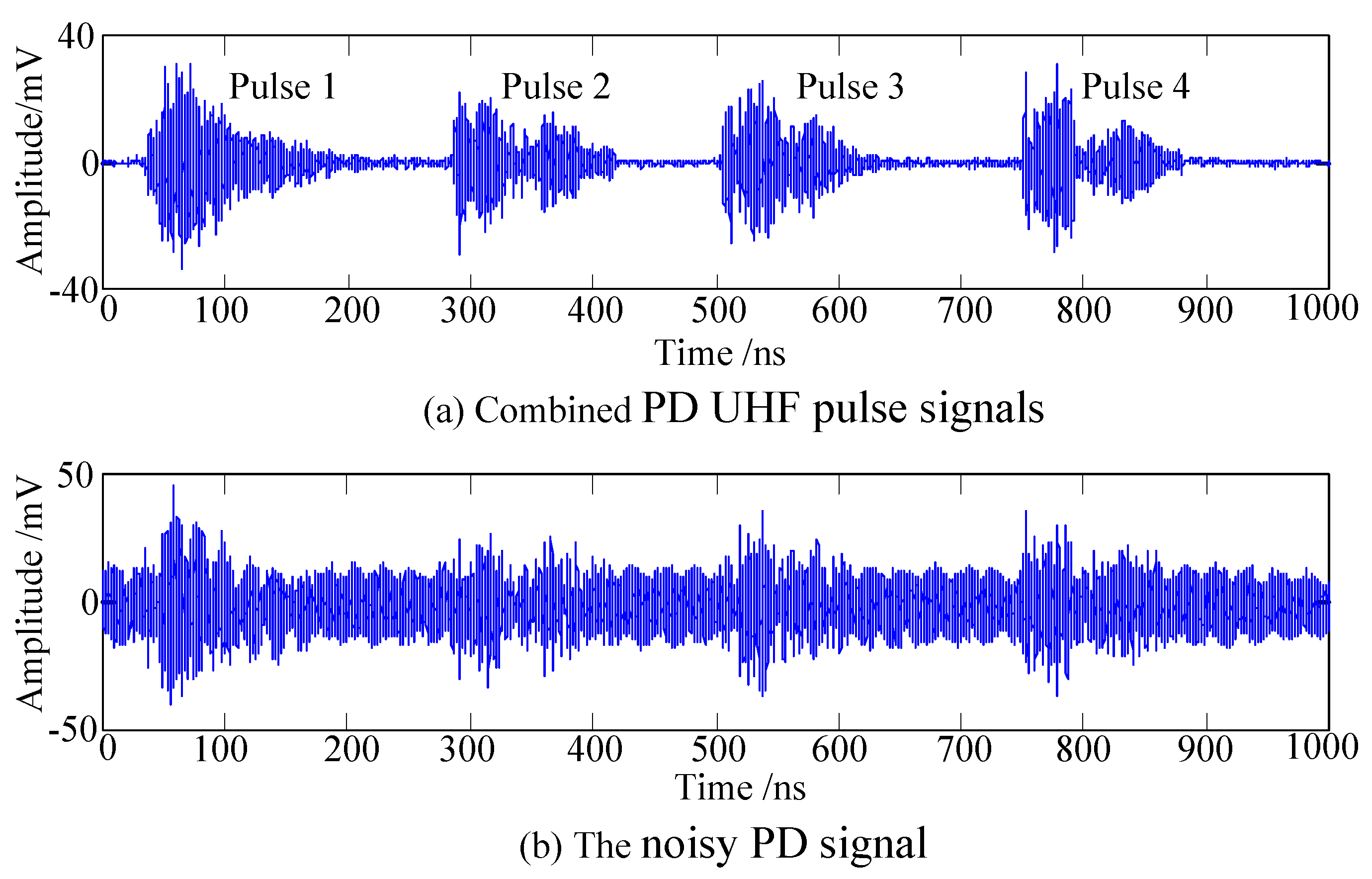
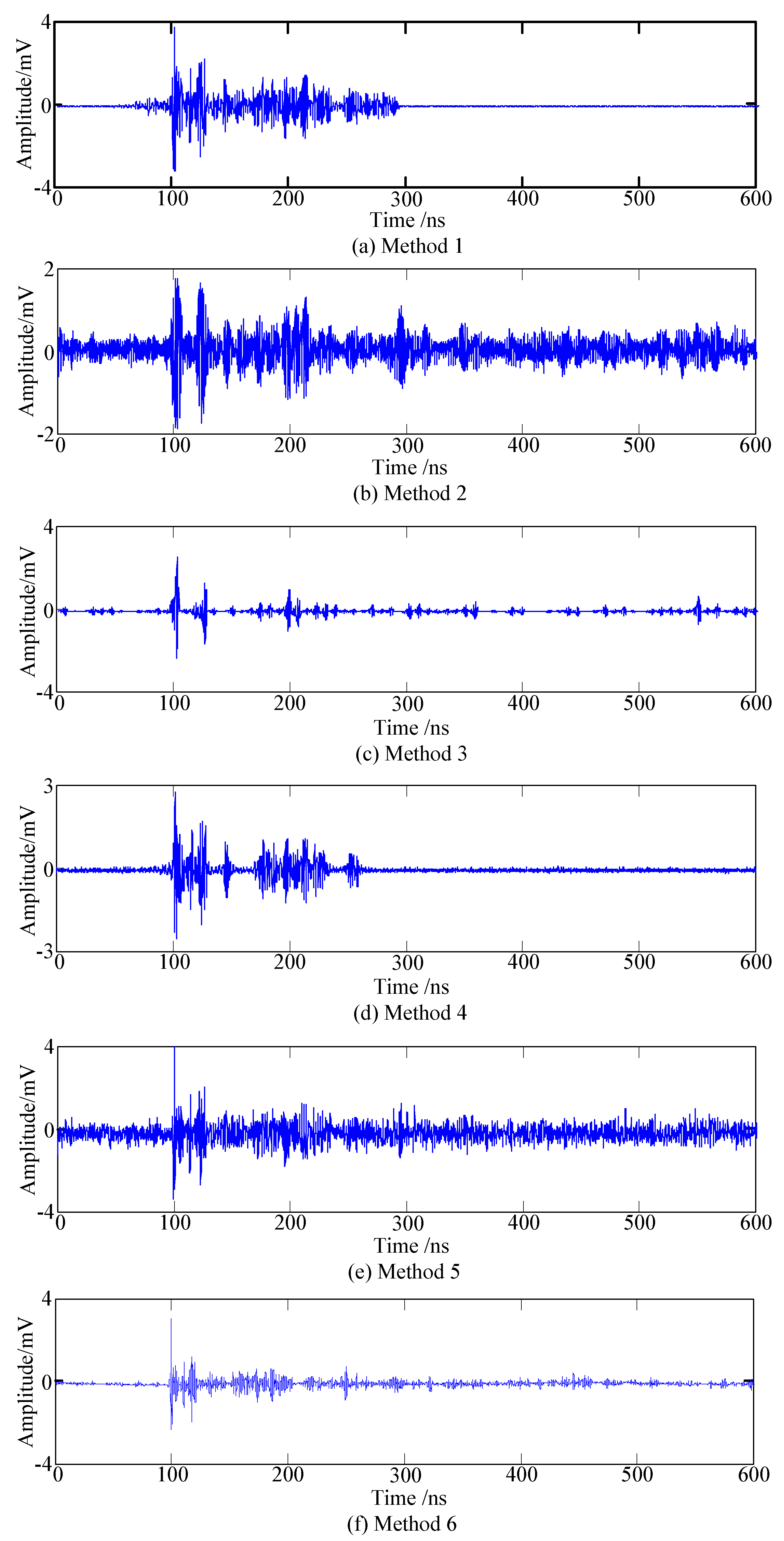
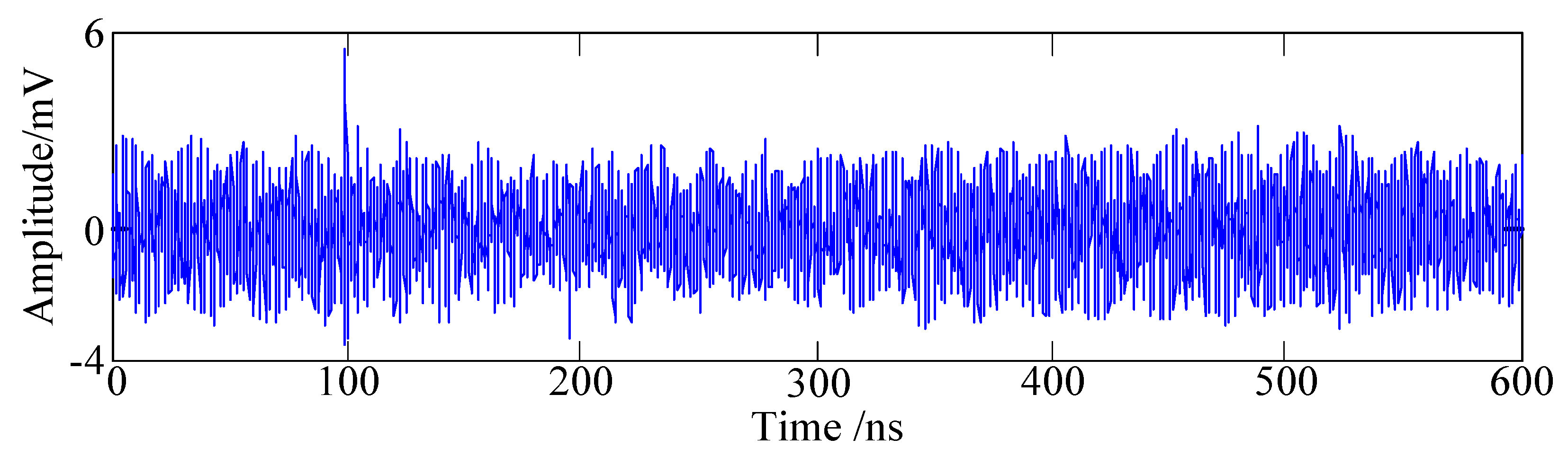
The live PD detection was performed on a 500 kV open-type substation in operation, as shown in Figure 11. The devices are the same as those for the simulation test in Section 3. Figure 12 shows the detected PD UHF signal with noise interference. The PD signal is seriously interfered by the background noise and has obvious distortion. Six methods in Table 2 were performed to de-noise the detected PD UHF signal in the field test. The de-noising results are shown in Figure 13.

Since the original PD UHF signal with no noise interference cannot be obtained in the field test, the evaluation method in Section 3.2 cannot be used to evaluate the de-noising performance. Hence, the evaluation indices of the noise suppression ratio and the amplitude attenuation ratio are proposed for evaluating the de-noising performance in the field test. The noise suppression ratio denotes the suppression effect of the PD UHF signal after de-noising. The de-noising effect is positively proportional to the noise suppression ratio. The amplitude attenuation ratio denotes the attenuation degree of the PD UHF signal after de-noising. The distortion degree is positively proportional to the amplitude attenuation ratio.

Table 4. De-noising performance evaluation results in field test.

De-Noising Method	Noise Suppression Ratio	Amplitude Attenuation Ratio/%	Computing Time/s
Proposed BSS	16.14	27.6	1.813
AF	8.91	67.4	0.893
AWT	13.22	51.3	1.141
RS	14.62	52.5	2.121
GSMT	10.87	28.3	6.212
UWT	12.01	37.6	1.485

shows the evaluation results of de-noising performance for various methods. The proposed de-nosing method can effectively suppress noise interference, and the amplitude attenuation of the de-noising PD signal is the smallest, compared with traditional methods. In addition, the proposed method can effectively reduce the calculation amount and computing time.

5. Conclusions

This paper proposed a novel PD UHF signal de-noising method, based on a single-channel blind source separation algorithm. This method utilizes the SVD calculation to convert the single-channel detected PD signals into multi-channel detected signals, and can effectively suppress the background noise in the PD UHF signals, combined with the JADE and l₁-norm minimization methods. The conclusions are as follows:

(1)

The submatrix of the SVD decomposition of the original PD signal can convert the single-channel detected PD signal into multi-channel PD signals; the underdetermined problem of blind source separation can be effectively solved.

(2)

The l₁-norm minimization method can effectively solve the large amplitude vibration problem after single-channel blind source separation, which is better for the subsequent signal processing and analysis.

(3)

Compared with traditional methods, the proposed method can effectively de-noise the Gaussian white noise and periodic narrow-band interference, and have small distortion.

The proposed method can be applied in the field partial discharge location and the insulation defect identification of HV apparatus. In addition, the field partial discharge location based on the proposed method will be studied in the future work.

References

1. Mor, A.R.; Heredia, L.C.; Munoz, F.A. Estimation of charge, energy and polarity of noisy partial discharge pulses. IEEE Trans. Dielectr. Electr. Insul. 2017, 24, 2511–2521. [Google Scholar] [CrossRef]
2. Wang, X.; Li, X.; Rong, M.; Xie, D.; Ding, D.; Wang, Z. UHF Signal Processing and Pattern Recognition of Partial Discharge in Gas-Insulated Switchgear Using Chromatic Methodology. Sensors 2017, 17, 177. [Google Scholar] [CrossRef] [PubMed]
3. Illias, H.A.; Tunio, M.A.; Bakar, A.H.A.; Mokhlis, H.; Chen, G. Partial discharge phenomena within an artificial void in cable insulation geometry: Experimental validation and simulation. IEEE Trans. Dielectr. Electr. Insul. 2016, 23, 451–459. [Google Scholar] [CrossRef]
4. Zhang, X.; Cheng, Z.; Gui, Y. Design of a New Built-in UHF Multi-Frequency Antenna Sensor for Partial Discharge Detection in High-Voltage Switchgears. Sensors 2016, 16, 1170. [Google Scholar] [CrossRef] [PubMed]
5. Sriram, S.; Nitin, S.; Prabhu, K.M.M.; Bastiaans, M.J. Signal denoising techniques for partial discharge measurements. IEEE Trans. Dielectr. Electr. Insul. 2005, 12, 1182–1191. [Google Scholar] [CrossRef]
6. Khan, S.Z.; Deheng, Z.; Xianhe, J.; Kexiong, T. A new adaptive technique for on-line partial discharge monitoring. IEEE Trans. Dielectr. Electr. Insul. 1995, 2, 700–707. [Google Scholar] [CrossRef]
7. Shang, H.; Lo, K.L.; Li, F. Partial Discharge Feature Extraction Based on Ensemble Empirical Mode Decomposition and Sample Entropy. Entropy 2017, 19, 439. [Google Scholar] [CrossRef]
8. Shetty, P.K.; Ramu, T.S. An Undecimated Wavelet Transform Based Denoising, PPCA Based Pulse Modeling and Detection-Classification of PD Signals. In Proceedings of the 17th International Conference on Pattern Recognition, Cambridge, UK, 26 August 2004. [Google Scholar]
9. Ma, X.; Zhou, C.; Kemp, I.J. Interpretation of wavelet analysis and its application in partial discharge detection. IEEE Trans. Dielectr. Electr. Insul. 2002, 9, 446–457. [Google Scholar] [CrossRef] [Green Version]
10. Lu, J.; Zhang, X.; Xiong, H. A New Method for Suppressing Periodic Narrowband Interference Based on the Chaotic van der Pol Oscillator. Int. J. Bifurc. Chaos 2015, 25, 1550120. [Google Scholar] [CrossRef]
11. Yuhui, Z.; Weirun, D.; Tianyun, L. A reverse separation method of suppressing periodic narrowband noise in partial discharge signal. Trans. China Electr. Soc. 2015, 30, 232–239. (In Chinese) [Google Scholar]
12. Majidi, M.; Fadali, M.S.; Etezadi-Amoli, M.; Oskuoee, M. Partial discharge pattern recognition via sparse representation and ANN. IEEE Trans. Dielectr. Electr. Insul. 2015, 22, 1061–1070. [Google Scholar] [CrossRef]
13. Liu, Y.; Zhou, W.; Li, P.; Yang, S.; Tian, Y. An Ultrahigh Frequency Partial Discharge Signal De-Noising Method Based on a Generalized S-Transform and Module Time-Frequency Matrix. Sensors 2016, 16, 941. [Google Scholar] [CrossRef] [PubMed]
14. Ashtiani, M.B.; Shahrtash, S. Feature-oriented de-noising of partial discharge signals employing mathematical morphology filters. IEEE Trans. Dielectr. Electr. Insul. 2012, 19, 2128. [Google Scholar] [CrossRef]
15. Ashtiani, M.; Shahrtash, S. Partial discharge de-noising employing adaptive singular value decomposition. IEEE Trans. Dielectr. Electr. Insul. 2014, 21, 775–782. [Google Scholar] [CrossRef]
16. Bell, A.J.; Sejnowski, T.J. An information-maximization approach to blind separation and blind deconvolution. Neural Comput. 1995, 7, 1129–1159. [Google Scholar] [CrossRef] [PubMed]
17. Amari, S.-I.; Cardoso, J.-F. Blind source separation—Semiparametric statistical approach. IEEE Trans. Signal Process. 1997, 45, 2692–2700. [Google Scholar] [CrossRef]
18. Amari, S.I.; Chen, T.P.; Cichoki, A. Stability analysis of adaptive blind source separation. Neural Netw. 1997, 10, 1345. [Google Scholar] [CrossRef]
19. Belouchrani, A.; Abed-Meraim, K.; Cardoso, J.F.; Moulines, E. A blind source separation technique using second-order statistics. IEEE Trans. Signal Process. 1997, 45, 434–444. [Google Scholar] [CrossRef]
20. Yang, Y.; Zhang, D.; Peng, H. Single-channel blind source separation for paired carrier multiple access signals. IET Signal Process. 2017, 12, 37–41. [Google Scholar] [CrossRef]
21. Wang, K.; Liao, R.; Yang, L.; Li, J.; Grzybowski, S.; Hao, J. Optimal features selected by NSGA-II for partial discharge pulses separation based on time-frequency representation and matrix decomposition. IEEE Trans. Dielectr. Electr. Insul. 2013, 20, 825–838. [Google Scholar] [CrossRef]
22. Rodriguez, A.; Laio, A. Machine learning. Clustering by fast search and find of density peaks. Science 2014, 344, 1492–1496. [Google Scholar] [CrossRef] [PubMed]
23. Luo, B.; Hancock, E.R. Structural graph matching using the EM algorithm and singular value decomposition. IEEE Trans. Pattern Anal. Mach. Intell. 2001, 23, 1120–1136. [Google Scholar] [Green Version]
24. Dai, D.; Wang, X.; Long, J.; Tian, M.; Zhu, G.; Zhang, J. Feature extraction of GIS partial discharge signal based on S-transform and singular value decomposition. IET Sci. Meas. Technol. 2017, 11, 186–193. [Google Scholar] [CrossRef]
25. Wu, H.C.; Huang, X.; Wu, Y.; Wang, X. Theoretical studies and efficient algorithm of semi-blind ICI equalization for OFDM. IEEE Trans. Wirel. Commun. 2008, 7, 3791. [Google Scholar] [CrossRef]
26. Asif, M.S.; Romberg, J. Fast and Accurate Algorithms for Re-Weighted l1-Norm Minimization. IEEE Trans. Signal Process. 2013, 61, 5905–5916. [Google Scholar] [CrossRef]
27. Kopf, U.; Feser, K. Rejection of narrow-band noise and repetitive pulses in on-site PD measurements. IEEE Trans. Dielectr. Electr. Insul. 1995, 2, 433–446. [Google Scholar] [CrossRef]
Figure 1. Schematic diagram of the JADE blind source separation algorithm.
Energies 11 00509 g001
Figure 2. Flow chart of single-channel blind source separation de-noising algorithm.
Energies 11 00509 g002
Figure 3. Simulation method of insulation defects.
Energies 11 00509 g003
Figure 4. Simulation test platform. GIS gas insulated switchgear; UHF, ultra-high frequency.
Energies 11 00509 g004
Figure 5. Schematic diagram of the simulation test platform.
Energies 11 00509 g005
Figure 6. Partial discharge (PD) UHF signals of the simulation tests.
Energies 11 00509 g006
Figure 7. Time–frequency distribution and clustering results of source signals.
Energies 11 00509 g007
Figure 8. Reconstructed virtual channel signals.
Energies 11 00509 g008
Figure 9. De-noised results using the blind source separation method.
Energies 11 00509 g009
Figure 10. De-noised results using traditional de-noising methods.
Energies 11 00509 g010
Figure 11. Field test platform.
Energies 11 00509 g011
Figure 12. The detected PD UHF signal in the field test.
Energies 11 00509 g012
Figure 13. De-noising results in field test.
Energies 11 00509 g013