Do Customers Choose Proper Tariff? Empirical Analysis Based on Polish Data Using Unsupervised Techniques

Abstract

Individual electricity customers that are connected to low voltage network in Poland are usually assigned to the most common G11 tariff group with flat prices for the whole year, no matter the usage volume. Given the diversity of customers’ behavior inside the same specific group, we aim to propose an approach to assign the customers based on some objective factors rather than subjective fixed assignment. With the smart metering data and statistical methods for clustering we can explore and recommend each customer the most suitable tariff to benefit from lower prices thus generate the savings. Further, the paper applies hierarchical, k-means and Kohonen approaches to assign the customers to the proper tariff, assuming that the customer can gain the biggest expenses reduction from the tariff switch. The analysis was conducted based on the Polish dataset with an hourly energy readings among 197 entities.

1. Introduction

Since the early days of the liberalization of the Electricity Market, there were many efforts worldwide aimed to investigate methodologies to form optimal tariffs based on customer usage data, derived from various clustering and classification techniques. Clustering techniques have become the main source of information for the development of the Demand Side Management (DSM) and Demand Response (DR) tools programs in the field of efficient use of electricity and tariff development [1,2]. These were also used to support energy suppliers and policy makers in developing strategies to act on the behavior of energy consumers, with the aim of shifting the demand from on-peak to off-peak hours. Classification techniques deliver means to identify groups of customers that fall into standardized load demand profiles. Besides flat and conventional tariffs, dynamic pricing and non-linear optimization models for the dynamics pricing based on time of use rate has appeared for the purpose of tariff recommendations [1,3]. Time of use, real time pricing, and spot price of electricity stand the basis for tariff modeling in competitive market [4].

The energy market liberalization in Poland is insufficient in comparison to other European countries and the improvement of its status would serve, among others, tariff abolition for individual users and households, dispersion of the sector’s property, and the development of modern infrastructure. Until now, only 3% of electricity users have changed the electricity supplier in Poland. The market has an oligopoly structure with state-owned companies representing nearly 90% of the market. Customers did not benefit from liberalization of the market. Moreover, while the EU countries are witnessing a resignation from feed-in tariffs, Poland is for the first time in history introducing feed-in tariffs, which are relatively high when considering the prices prevailing in the Polish electricity market. The effects on the economy of a feed-in tariff policy mechanism are well investigated by Ponta et al. [5].

The demand side of the retail electricity market in Poland consists of couple of end-users groups. In total, there are approximately 17.05 million of end-users and among them 90.3% (15.4 million) are the customers belonging to G tariff group, with a majority of household consumers (over 14.5 million). The rest of end-users are the customers who belong to A, B or C tariff groups. The first two groups that is A (top, strategic clients) and B (big, key clients) include the customers connected to high and medium voltage grids, whereas group C contains customers that are supplied from the low voltage grid. All three groups are consuming electricity to maintain their business activity and they are referred as commercial customers [6].

A very important issue in the Polish electricity market, since the changing that took place the late 1990s, is the collection of detailed information on electricity consumption of individual consumers of A, B and C tariff groups, supplied from different voltage levels. Knowledge of load schedules based on hourly measurement has become the basis for electricity sales forecasting and customers clustering.

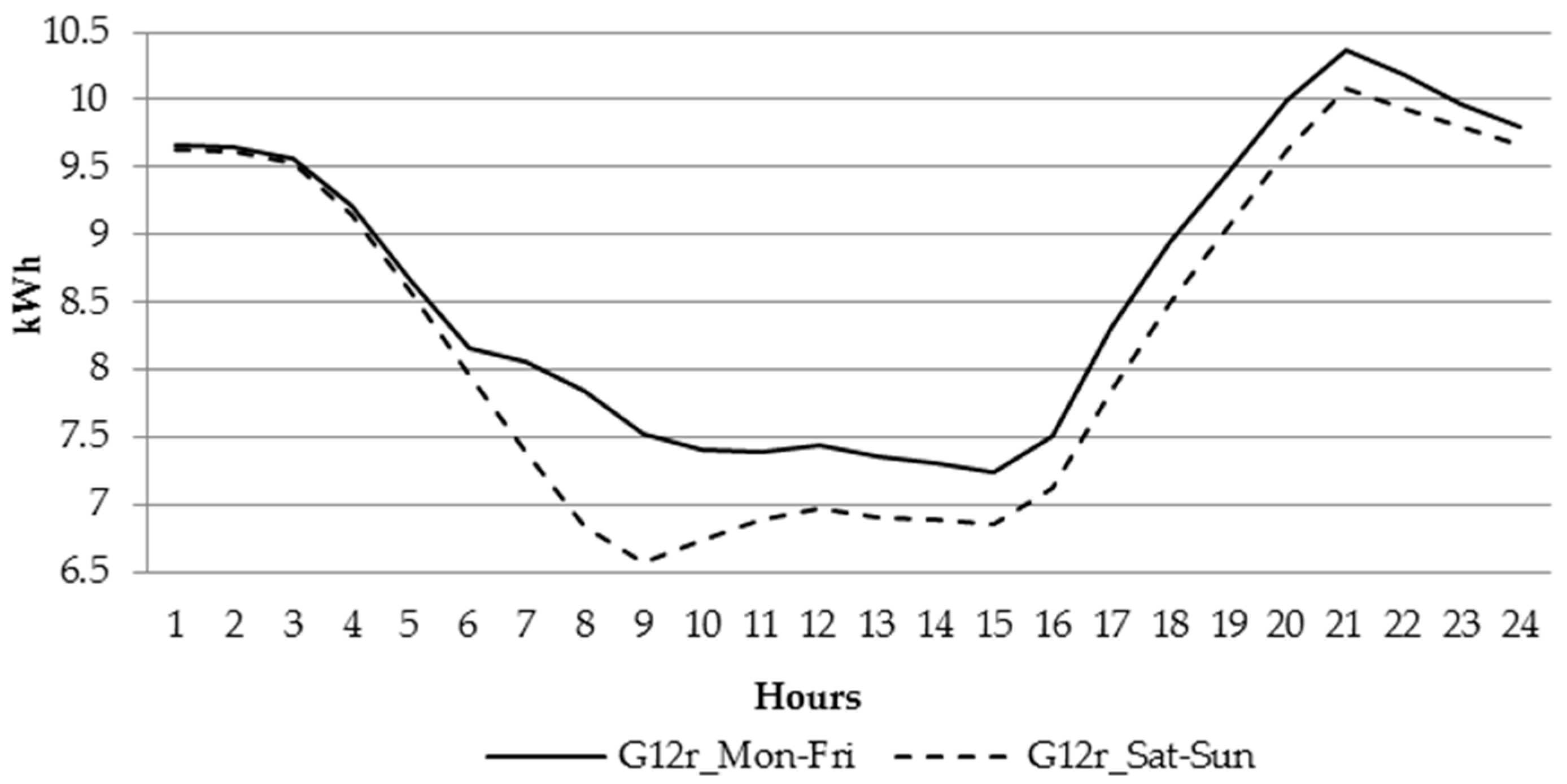
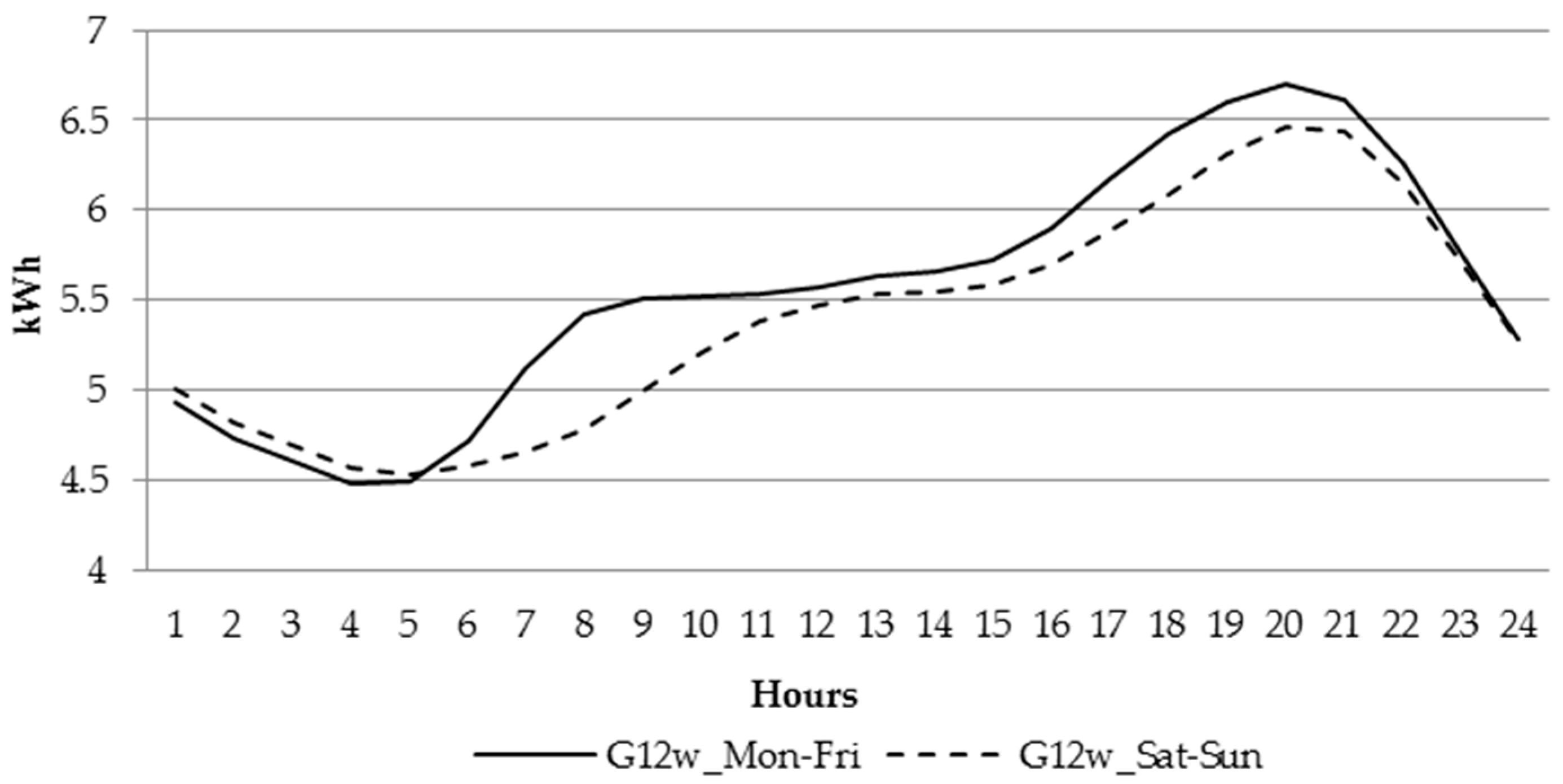
For the households powered at low voltage, the business entities have created couple of different tariff groups, which differ by time zone (single or two time zone meters) and whether electricity is used for heating or not. The most generic household tariff group is G11—customers having single-time zone meters with a single electricity rate per KWh (Kilowatt hour). The remaining tariff groups, G12, G12r, G12w, are time and weekdays. G12 is effective between 10 p.m. and 6 a.m. and between 1 p.m. and 3 p.m., while G12w is additionally effective during the weekends (between 10 p.m. on Friday and 7 a.m. on Monday). G12r is effective seven days a week between 10 p.m. and 7 a.m. and between 1 p.m. and 4 p.m.

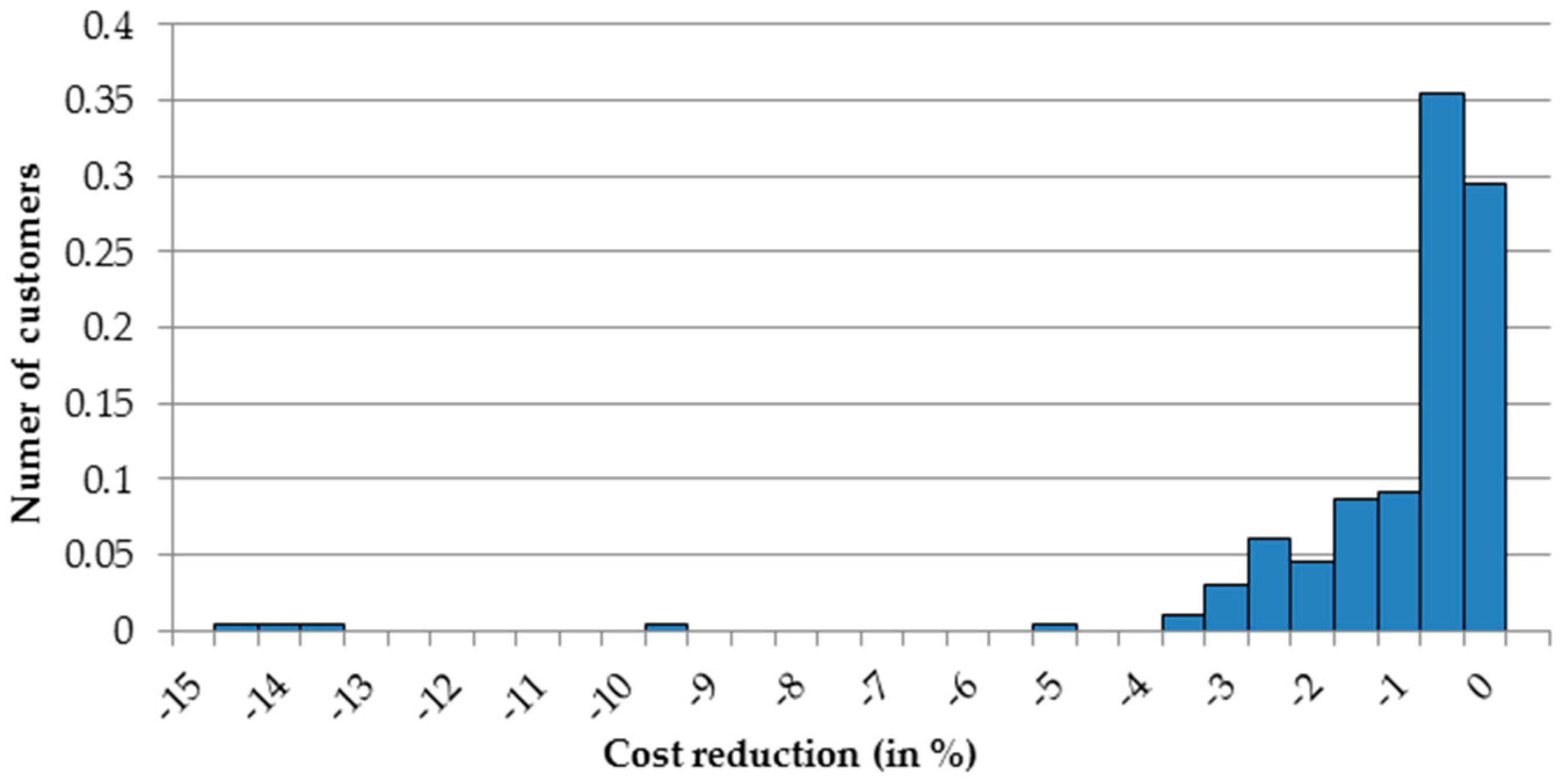
In this article, we aim to explore the individual characteristics of electricity usage and recommend to each customer the most suitable tariff to benefit from lower prices, thus optimize the expenses. Based on the 197 individual customers belonging to tariff group G11 we observed that in the analyzed period between 1 January and 31 December 2015, 75% of them would have lower bills if they were moved to G12w tariff group, and further 6% of them were moved G12r tariff. Only 19% of the analyzed entities should stay in their current G11 tariff. Such observation is important for both, the customers and electricity providers. The first ones benefit from lower prices, while the latter ones can better balance the demand with less instability in the system.

When overwhelming majority of the customers belongs to one tariff with a lot of variance inside the group, it creates number of problems including proper forecasting to meet the Demand Side Response (DSR) by the electric entities, not mentioning the stability of the whole grid [7]. Of course, daily energy consumption does not depend only on customer tariffs composition, but it is influenced by number of external factors, which are related to weather conditions, atmospheric phenomena, and specific days [8,9]. In this context, there is a need for an objective approach to increase the efficiency and effectiveness of the grid management and operations by breaking down mass markets into groups of consumers that have clearly similar patterns of behavior. This can be supported by statistical clustering methods to formulate valid and meaningful clusters based on the available hourly measurements data. For instance, Weron [1] provides a review of several methods and applications to forecast and cluster hourly electricity price data according to their similarity. With the increased stream towards the deregulation of the market, the forecasting of electricity demand and price has emerged as one of the major research fields in financial and electrical engineering [4].

The total demand observed at the electric utility level is a sum of individual demands. Previous hourly electricity usage of strategic, key and business customers are read directly from different measurement devices and suitable used to forecast future demand with a high accuracy [10]. When considering a large number of customers that are powered at low voltage level, especially households, hourly measuring and recording devices state a great deficiency. Both future demand and preliminary customer settlement are determined based on tariff groups load shape. In this case, similar structure of energy demand will determine the number of clusters. Statistical and engineering techniques [11,12,13,14], time series [10,15,16], and neural networks [14,17,18] are used to assist load profiling.

Based on the literature query, there is a clear and more noticeable research trend that is focused on various aspects related to segmentation of the electricity end users. For instance, an application of k-means clustering method for the purpose of grouping daily load profiles of residential users was reported in many works [16,19,20,21]. The load profiles as result individual residential customers segmentation have been investigated by Al-Wakeel, A. and Wu J. [22,23]. A comparison among clustering algorithms for non-residential electricity customer classification, including hierarchical clustering and Kohonen self-organizing map (SOM) was analyzed, among others, by Chicco et al. [24].

Given the availability of usage data from 197 individual entities we have investigated the potential of unsupervised clustering to automatically infer from the electricity usage data. The goal is to characterize the electricity consumption patterns based on the segmentation of the customers by features considered to be correlated to the consumption, and thus to identify the most suitable tariff plan.

2. Dataset Characteristics

2.1. Customer Characteristics

This study was prepared based on historical data representing energy consumption observed at 197 entities, including households and small business customers, in Mazovia, Poland. The data set included hourly data that covered the period between 1 January 2015 and 31 December 2015. As depicted in Figure 1, for the time series aggregated for 197 entities a number of annual, weekly, and daily seasonal cycles was observed. For instance, the daily load curves have different shapes depending on the day (workday, Saturday, Sunday, or holiday) and the season. Figure 2 presents weekly profile with relatively low electricity consumption during night, clearly defined peaks in the evenings, and slightly smaller peaks in the late morning. Finally, the consumption is significantly lower during the weekend days as compared to working days.

Although the daily shapes of the load for the whole group of 197 customers are smooth we observed quite different characteristics of individual households and entities regarding the volume and volatility. To analyze the hourly volatility a box and whisker plots were prepared for two customers using load data for the whole year—one with quite stable load profile and the second one with highly volatile characteristics, see Figure 3 and Figure 4 for details.

The whiskers denote the minimum and the maximum value for each hour and the box contains 50% of the data (bottom edge reflects 25th quartile and top edge 75th quartile, while the line in the middle of the box is the median). For instance, one of the entities, as shown in Figure 3, on average consumes 10 kWh in each hour, while the volatility is rather low, regardless day or night. On the other side, the other household, as shown in Figure 4, can be characterized as the one using, on average, only 0.1 kWh in each hour, however, the volatility of the load is very high.

Depending on the tariff plan, the customers can benefit from lower prices per kWh if the usage falls between certain time zones. In Figure 5 the prices for G11, G12r and G12w are presented. G11 tariff has the fixed price of 0.30 PLN/kWh. G12r tariff plan has lower rate of 0.18 PLN/kWh between 10 p.m. and 7 a.m. and between 1 p.m. and 4 p.m., while the higher rate of 0.40 PLN/kWh is applicable outside these windows. G12w has lower rate of 0.24 PLN/kWh during the weekends and Monday–Friday between 10 p.m. and 6 a.m. and between 1 p.m. and 3 p.m., while the higher price of 0.36 PLN/kWh is applicable outside these windows.

All of the customers were assigned to G11 users group, which is single-time zone tariff with flat price per kWh, irrespective of time and volume. However, in the analyzed data, we could easily find the entities matching other tariffs groups. For instance, Figure 6 presents average usage observed at the entities that fit to the characteristics of G11 tariff since the load profile is stable between 9 a.m. and 9 p.m. with low consumption in the evening hours, regardless of the day of the week.

In Figure 7 there is another example of the entities with the load characteristics matching G12r tariff group. The usage valley is observed between 9 a.m. and 4 p.m., while the night hours are quite occupied, irrespective day of the week.

Finally, Figure 8 presents average usage observed at the entities that fit to the load shape matching G12w tariff plan.

Based on the 197 customers belonging to G11 tariff group, we observed that in the analyzed period between 1 January and 31 December 2015, 75% of them would have lower bills if they were moved to G12w tariff group, and a further 6% of them were moved G12r tariff. Only 19% of the analyzed entities should stay in their current G11 tariff. As presented in

Table 1. Simulation of households electricity consumption cost based on different tariff group rates.

Tariff Group	Electricity Consumption Costs [PLN]	Electricity Consumption Cost [in %]
Electricity cost in G11	2,401,545.00	100.00
Electricity cost in G12/G12r/G12w	2,358,987.84	98.23
Customer savings due to switching	42,557.16	1.77
Electricity Consumption Cost After Switching the Tariff	Electricity Cost [PLN]	G11
G11 tariff group	36,764.50	0
G12r tariff group	265,843.50	10,314.65
G12w tariff group	2,098,937.00	32,242.51
Total	2,401,545.00	42,557.16

, the summarized electricity consumption cost for all the 197 customers reaches 2,401,545 PLN. If the customers would chose appropriate tariff the electricity cost would amount to 2,358,987 PLN what would give them savings of about 42,557 PLN (1.77%). The savings are mainly due to the switching the tariff from G11 to G12w—32,242 PLN, and from G11 to G12r—10,31 4PLN.

A distribution of percentage improvement due to switching the tariff group is shown in Figure 9. About 97% of the entities would benefit up to 4% due to the cost reduction and only three customers would lower their electricity bills by more than 10%.

2.2. Features Definition for Segmentation

This study was prepared based on historical energy consumption data from 197 Polish entities. For each entity, the dataset included hourly data covering the time window between 1 January 2015 and 31 December 2015. Beside the daily energy consumption characterized by the day type (weekday and weekend), hour of use and season, many other features were considered, such as trend decomposition, base load historical features, and some statistical transformations of the base load.

From the data we extracted 91 features where their definitions were taken from [25,26,27]. The features were depicting consumption characteristics like the minimum, mean and maximum consumption in different time windows during the day (day type, time-zone), ratios (daytime-ratios and ratios between different days), statistical features, including variance, auto-correlation, and other simple statistical measures, and, finally, different temporal characteristics like peaks loads, breaching certain consumption levels, or temporal load deviations.

3. Unsupervised Techniques

3.1. Hierarchical Clustering

The aim of cluster analysis is to group objects according to their similarity on the variables. It is often called unsupervised classification, meaning that classification is the ultimate goal, but the classes (groups) are not known ahead of time. One of the earliest clustering algorithms is called hierarchical algorithm. At the beginning all of the observations are either in a single cluster or all of the objects are in their individual cluster, then we start fusing objects into groups until every single case is in one single group (cluster) or in the inverse order when splitting the cases. This process can be viewed using a tree diagram called dendrogram. Hierarchical methods for clustering can be basically divided into agglomerative and divisive approach. The most used approach is Hierarchical Agglomerative Clustering (HAC); it starts with one cluster and one observation in its own cluster and iteratively merge clusters until all the observations belong to one cluster. Bottom up approach is followed to merge the clusters together and the vertical heights of the dendrogram are used to decide about their number, using Euclidean distance formula. Not all clustering is done using Euclidean distance, the most useful agglomerative clustering method called Wards [28] fuses the objects together using the smallest increase in the error after fusing two clusters. Ward’s method starts with $\mathrm{n}$ clusters of size $1$ and continues by aggregating the observations until all of them are included into one cluster. The general concept of divisive clustering algorithm essentially is that the process starts at the root with all items in one big macro cluster, and then recursively splits the higher level cluster to build the dendrogram, until finally every single item becomes a singleton cluster. The method is called divisive analysis (DIANA) [29]. It is a top-down approach and can be considered as a global approach and more efficient when compared to the agglomerative clustering algorithm.

3.2. K-Means Clustering and Multidimensional Scaling

K-means algorithm [30] is an optimization clustering technique that classifies given data set through a certain number of K clusters, specified by the user. Each cluster has a center called centroid. Given K, the K-means algorithm works as follow: for given data set points $D=\left(x_1,\dots ,x_n\right)$, there are some points near the centroid of their clusters, others are far apart. K-means method assumes a certain number K of clusters ahead, with unknown centers $\left({\mu }_1,\dots ,{\mu }_k\right)$, and tries to minimize the distance between the assigned points and their cluster center using the square of Euclidean distance. This is done for all the clusters according to the formula:

$$\min {{\displaystyle \sum }}_{j=1}^K{{\displaystyle \sum }}_{\begin{array}{c}i: x_i is\\ assigned to j\end{array}}d\left(x_i,{\mu }_j\right)=\min {{\displaystyle \sum }}_{j=1}^K{{\displaystyle \sum }}_{i=1}^n{a}_{i,j}\Vert x_i-{\mu }_j\Vert {}^2,$$

(1)

where, $a_{i,j}$ is a binary coefficient with a value equal to one or zero depending whether $x_i$ is assigned to the cluster j or not.

The objective function depends only on assigned points and the position of the cluster center ${\mu }_j$ and can be solved iteratively in two steps with respect to all $a_{i,j}$ and ${\mu }_j$. First the algorithm chooses optimal $a_{i,j}$ for fixed ${\mu }_j$. This is can be solved by assigning $x_i$ to the nearest ${\mu }_j.$ Second K-means determines the optimal centers ${\mu }_j$ for fixed assignment $a_{i,j}$ with respect to ${\mu }_j$ .This is can be done minimizing the object function using gradient descent approach.

Unfortunately, the iterative scheme of K-means does not guarantee converging to a global minimum of the objective function. It may also converge to values that are not optimal, depending on the choice of the initial cluster centers. Despite these deficiencies, the K-means algorithm remains very popular thanks to its quickness to converge.

Multidimensional scaling (MDS) is a method that presents the similarity of cases in a set of multivariate quantitative data. The idea behind MDS procedure is to project points or objects from a higher to a lower dimensional space in a manner that preserve as much as possible the distances between individual multivariate observations. In general, having a vector representation of n data points (objects) $X=\left[x_1,x_2,\dots \dots x_n\right]$ in d-dimensional space $x_i\in {ℝ}^d$ MDS attempts to map a vector representation Y data points (objects) $Y=\left[y_1,y_2,\dots \dots y_n\right]$ in p-dimensional space $y_i\in {ℝ}^p$, ($p<d$), such that if $d_{i,j}^{\left(Y\right)}$ denotes the Euclidian distance between $y_i$ and $y_j$, then the distance matrix $D^{\left(Y\right)}$ is similar to the dissimilarity matrix $D^{\left(X\right)}$. Two fundamental types of MDS are metric and non-metric. Metric MDS expects that the underlying data is quantitative and that it requires a useful relationship between the inter-point distances and the given dissimilarities. Non-metric MDS assumes that the data is qualitative and having some ordinal importance to provide configurations that enable assigning the order of the dissimilarities. These dissimilarities might be non-Euclidian or even non-metric. Distances are however metric measures in the established vector space. In this paper, one classical metric MDS, referred to as classical scaling that minimizes the objective function will be applied:

$$\underset{Y}{\min }{{\displaystyle \sum }}_{i=1}^n{{\displaystyle \sum }}_{j=1}^n{\left(d_{i,j}^{\left(X\right)}-d_{i,j}^{\left(Y\right)}\right)}^2,$$

(2)

where $d_{i,j}^{\left(X\right)}=\Vert x_i-x_j\Vert$ and $d_{i,j}^{\left(Y\right)}=\Vert y_i-y_j\Vert$. To find the minimum of the objective function, most implementations of MDS algorithms use standard gradient methods [31].

3.3. Self-Organizing Maps

Self-organizing maps SOM or self-organizing features map outline a kind of artificial networks using unsupervised learning technique that allow us to visualize multi-dimensional data in fewer (one or two) dimensions. The success of SOM is due to the fact that they allow for deriving a map of very high dimensional space, and the learning of such networks does not require supervision. In other words, they carry out the clustering of such space while building their two-dimensional illustration. Self-organizing networks are composed of two layers: the input layer and the output layer, also called the competition layer, which is usually a two- or one-dimensional array of neurons. The array of neurons has usually a rectangular or hexagonal grid.

Unlike other types of artificial neural networks, self-organizing networks do not have any hidden layer. Each competitive layer is connected to all input layer neurons. Also, each output neuron has as many weighting factors as there are network inputs. SOM belongs to one-way networks, so it does not include feedback loops or cycles.

A self-organizing map is built of components called nodes or neurons affiliated with each node, are away vector having the same dimension as the input data vectors and a position in the map space. The standard form of nodes is a two dimensional having regular spacing in a hexagonal or rectangular lattice. It was observed that SOM with a small number of nodes arrange data in a way that is similar to K-means, while the larger SOM transform data in a way that is fundamentally different. SOM approach with a small number of nodes can be thought of as a constrained version of K-means clustering [32]. Neurons of the first layer do not make any data transformations, and they only have to send out all the values introduced to the network’s inputs to the competitive layer. There, only the second layer neurons calculate the similarity of their weights vector $w_j=\left\{w_{ji}:j=1,\dots N;\mathrm{i}=1,\dots ,D\right\}$ to the input values vector $x=\left\{x_i:i=1,\dots ,D\right\}$, where $D$—presents the input space, $x_i$—the i-th value of the input value vector, $w_{ji}$—is the j-th value of the weight of the i-th neurons competition layer, $N$—is the total number of neurons. Finally, the discriminant function is formulated as the squared Euclidean distance between the input vector $x$ and the weight vector $w_j$ for each neuron j:

$$d_j\left(x\right)={\displaystyle \sum }_{i=1}^D{\left(x_i-w_{j,i}\right)}^2.$$

(3)

In SOM, a learning competitive algorithm is used; this means that after presentation of the input pattern (training vector $x$), not all neurons, as in other types of networks, modify their weight. Neurons compete with each other to become a winning neuron. The winner is the one whose weight vector is the closest (the smallest distance) to the presented input pattern. A topological neighborhood function for the neurons in the SOM can be adopted as:

$$T_{j,WIN}=\exp \left(\frac{-r_{j,WIN}^2}{2{\sigma }^2}\right),$$

(4)

where $r_{j,WIN}$ is the lateral distance between neurons j and, and the winner neuron the declared winning neuron $WIN$. A special feature of the SOM is that the size $\sigma$ of the neighborhood radius needs to decrease with time. A popular time dependence is an exponential decay: $\sigma \left(t\right)={\sigma }_0\exp \left(-\frac{t}{T_{\sigma }}\right)$, where ${\sigma }_0$ is the width of greed (lattice) at time zero, t state the current time step, and $T_{\sigma }$ is the time constant. The value of $T_{\sigma }$ depends on ${\sigma }_0$ and the chosen number of iterations for algorithm.

The learning of the SOM is of an iterative nature, which implies that the input data set is repeatedly presented during subsequent training epoch. Initially, the weight of the competitive layer neurons takse random values, which usually oscillate around zero. During the learning process, they gradually become similar to the data values that are presented at the network input. The SOM network learning basic algorithm (modification of weights) has the form:

$$\Delta w_{ji}=\eta \left(t\right)·T_{j,WIN}\left(t\right)·\left(x_i-w_{j,i}\right).$$

(5)

The time (epoch) $t$ dependent learning rate $\eta \left(t\right)={\eta }_0\exp \left(-\frac{t}{T_{\eta }}\right)$, and the updates are applied for all training patterns $x$ over many epochs. Repeated presentations of the training data leads thus to topological ordering. Two phases of the adaptive process can be specified: ordering or self-organizing phase with topological ordering of the weight vectors. The second converge stage, during which the feature map is fine-tuned and the statistical quantification of the input space is presented.

4. Clustering Results

The clustering was based on 91 features, as referenced in Section 2.2, and these were extracted for each of the entities. For each of 197 entities belonging to tariff group G11 we assigned a targeted tariff group, that is group matching customers’ electricity usage characteristics and resulting in lower bills when comparing to the current G11 tariff plan. We observed that in the analyzed period between 1 January and 31 December 2015, the following structure, as presented in

Table 2. Targeted customers tariff groups.

Targeted tariff	Initial Tariff—G11
	No. of Entities	% of Entities
Targeted tariff—G11	38	19%
Targeted tariff—G12r	12	6%
Targeted tariff—G12w	147	75%
Total	197	100%

, would be recommended to customers. The new structure was used to verify the results of clustering in terms of the accuracy and the proper assignment to each group.

4.1. The Results of Hierarchical Clustering

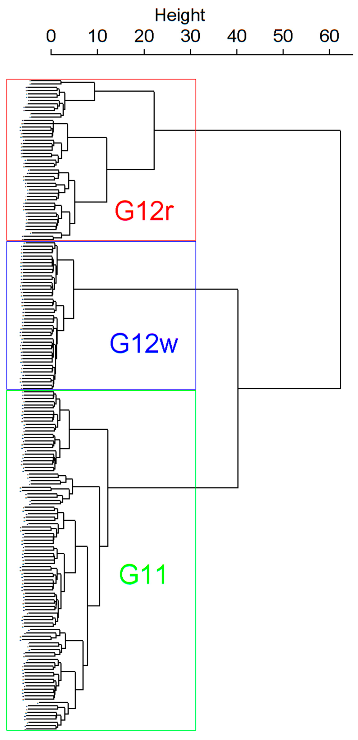
The outcome of Ward’s method application with the Euclidean distance measure is depicted as dendrogram in Figure 10.

The height of each edge of the dendrogram is proportional to the distance between the joined groups. As shown in Figure 10, two groups are distinctly separated from each other, and then one of them is further divided into two groups. Such partitioning can be used to determine the number of clusters in the data—in this case, three separate customers groups can be proposed. In the case of underlying data, we could observe that majority of entities would be assigned to G11 group that is presented in green in the figure. Next to it we have customers matching to G12w group specifics, presented in blue, and finally, there is a group presented in red, which includes the entities matching G12r characteristics.

4.2. The Results of K-Means Clustering and Multidimensional Scaling

The goal of the experiment is to discover similarity among the profiles by dividing the data into $k$ disjoint clusters, so that observations of the same cluster are close to each other and objects of different clusters are dissimilar. The output of a clustering is the list of clusters and the objects assigned to each clusters. To draw conclusions it is recommended to create a graphical representation that describes the objects with their surroundings, and showing the whole clusters. Such a chart was constructed using so-called CLUSPLOT [29] to visualize the outcome of the k-means algorithm. 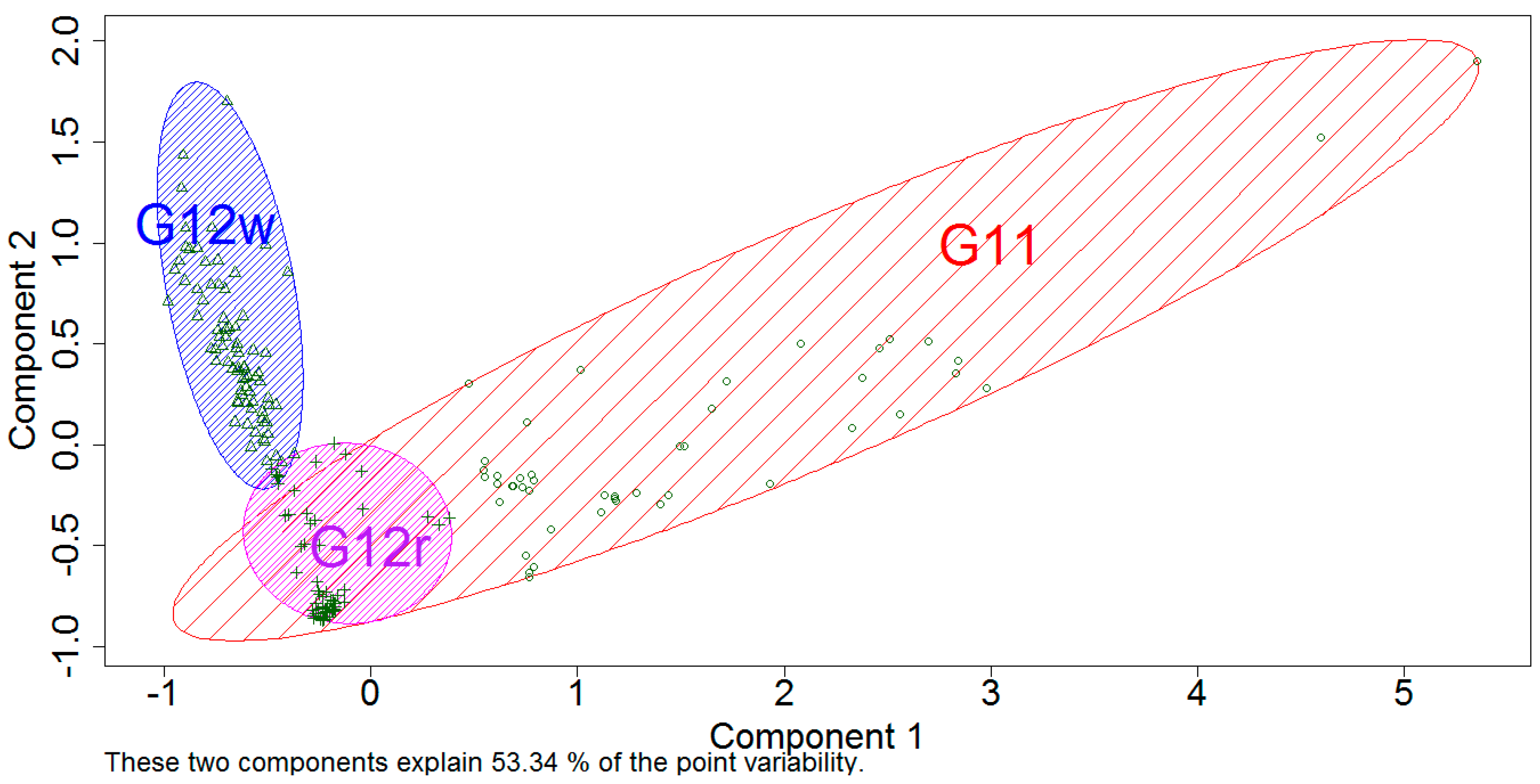For datasets with high dimensions, a reduction technique was applied before the plot was constructed, following the guidelines described in Section 3.2. The MDS method propose components, such that the first component accounts for as much variability as possible, the second component accounts for as much of the remaining variability as possible. This is the base for CLUSPLOT, which uses the outcome of MDS partition and the original data to produce Figure 11. The ellipses are constructed based on the average values of the components and the covariance matrices of each cluster. The cluster size is established in a way that it contains all of the points (entities) that are assigned by the technique. This justifies that there are always objects located on the boundary of each ellipse [33].

In this study, we tested several dissimilarity measures; however, in the Figure 11, we show the results of the Euclidean distance application what resulted in 53.34% of the point variability explained. The measures could explain less the point variability and were not considered for publication.

On the left in the picture (marked in blue) there is a group of customers matching G12w characteristics. Below G12w we have the circle area represented by G12r group, while the largest area of the oval shape is specific to G11 tariff group.

4.3. The Results of Self-Organizing Maps

SOM visualizations are made up of multiple nodes. Typical visualizations are heatmaps showing the distribution of a variable across the SOMs. An interesting interpretation of SOMs can be found on http://en.proft.me blog where author compares the SOMs to the place full of people and were each person in the room holds a colored card representing age—the result would be a SOMs heatmap. People of similar age would be aggregated in the same area.

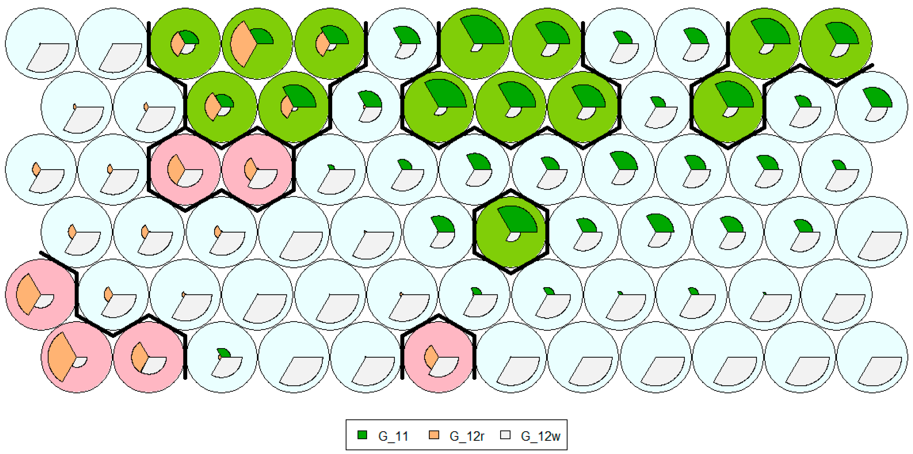
The SOMs consists of a set of codebook vectors that are arranged together in a topological structure, in a form of one-dimensional line or a two-dimensional grid. The role of the codebook vectors is to represent points within the domain, whereas the topological structure applies an ordering between the vectors during the training phase. The outcome is a low dimensional projection or approximation of the underlying domain where the clusters can be extracted and visualized. In our case, we have visualized SOM clusters with targeted mapping (optimal tariff group assignments), and have derived the structure presented in Figure 12. From the figure, we can see that majority of the nodes is assigned to G12w tariff group, six nodes are assigned to G12r, while the remaining nodes, presented in green, represent G11.

4.4. Evaluation of Clustering Techniques

To evaluate the accuracy of clustering techniques, their classification capability was validated. In other words we verified the correctness of the assignment to each cluster by checking against the targeted tariff groups. The positive verification was when the customer from the initial G11 tariff was assigned to the targeted group of G11, G12r, or G12w, and what would bring the customer financial benefits.

The accuracy is the most popular measure of classification capabilities. We can represent classification results as a contingency matrix $A$, with $A_{i,j}$ for $i,j\in \overrightarrow{t}=\left\{t_1,\dots ,t_k\right\}$ where $k$ is the number of possible target values, and $A_{ij}$ is the number of times that a data point with true label $t_i$ was classified as label $t_j$. Then accuracy is defined as follows:

$$\mathrm{Accuracy}=\frac{{{\displaystyle \sum }}_i{A}_{i,i}}{{{\displaystyle \sum }}_i{{\displaystyle \sum }}_j{A}_{i,j}}.$$

(6)

The accuracy formula is acceptable unless we observe high class imbalance in the data. Say, a classification task where 95% of data points are from class A, and 5% from class B. A faulty classifier that assigns the majority class label to all points will lead to 95% accuracy (seemingly very good) but is completely uninformative. When the distribution of class labels is skewed, the accuracy may become a poor evaluation measure. If there are only two labels, there are variety of choices for evaluation that have been developed through investigation of detection problems, including F-measure and ROC curves.

Read and Cox [34] proposed the use of balanced error rate (BER) or balanced accuracy (BAC), which are as follows:

$$BAC=1-BER=\frac{1}{k}{\displaystyle \sum }_i\frac{A_{i,i}}{{{\displaystyle \sum }}_j{A}_{i,j}}.$$

(7)

This is one minus the average recall (correct predictions of a class/true instances) treating each class evenly, regardless of its class membership.

The summary results in the form of classification matrices, for all of the clustering techniques, are presented in

Table 3. Classification matrices for: (a) hierarchical clustering, (b) k-means clustering, and (c) supervised clustering.

(a)
	Targeted Tariff
Clustering tariff		G11	G12r	G12w
	G12r	2.63% (1)	58.33% (7)	27.89% (41)
	G11	97.37% (37)	41.67% (5)	41.50% (61)
	G12w	0% (0)	0% (0)	30.61% (45)
	Total	100% (38)	100% (12)	100% (147)
(b)
	Targeted Tariff
Clustering tariff		G11	G12r	G12w
	G12r	2.63% (1)	66.66% (8)	25.85% (38)
	G11	92.10% (35)	25.00% (3)	31.30% (46)
	G12w	5.27% (2)	8.34% (1)	42.85% (63)
	Total	100% (38)	100% (12)	100% (147)
(c)
	Targeted Tariff
Clustering tariff		G11	G12r	G12w
	G12r	7.90% (3)	25.00% (3)	4.76% (7)
	G12w	71.05% (27)	66.67% (8)	79.60% (117)
	G11	21.05% (8)	8.33% (1)	15.64% (23)
	Total	100% (38)	100% (12)	100% (147)

. The columns represent the targeted tariffs (or the optimal one)—resulting in lower bills when comparing to the current G11 tariff plan, while the rows represent the tariffs derived from the clustering. The data are presented as percentages and frequencies (in brackets).

Based on the Table 3, the accuracy, according to Equations (6) and (7), for each of the clustering techniques was calculated, as shown in

Table 4. Classification accuracy.

Technique	Accuracy	BAC
Hierarchical clustering	45.2%	37.8%
K-means clustering	53.8%	32.8%
Supervised clustering	65.0%	58.1%

.

4.5. Assessment of Similarity between Clusterings

The Jaccard’s and Rand’s indices are one of the most frequently used similarity measures, in particular, often applied for data clustering. In general, the Jaccard’s index is relatively conservative, while the Rand’s index is relatively optimistic [35].

From a mathematical standpoint, those indexes are related to the accuracy, but are applicable even when class labels are not used. Generally, for two clusterings of the same data set, those measures calculate the similarity statistic that is specified of the clusterings from the co-memberships of the observations. Basically, the co-membership is defined using the pairs of observations that are clustered together, and the details for both measures are as follows:

$$Jaccard=\frac{n_{1,1}}{n_{1,1}+n_{1,0}+n_{0,1}},$$

(8)

$$Rand=\frac{n_{1,1}+n_{0,0}}{n_{1,1}+n_{1,0}+n_{0,1}+n_{0,0}},$$

(9)

where $n_{1,1}$ is the number of observation pairs where both observations can be found in both clusterings, $n_{1,0}$ is the number of observation pairs where the observations can be found in the first clustering but not in the second, $n_{0,1}$ is the number of observation pairs where the observations can be found in the second clustering, and finally, $n_{0,0}$ the number of observation pairs where neither pair can be found in either clustering [35].

The results of similarity assessment are presented in

Table 5. Similarity assessment using Jaccard’s and Rand’s measures.

Jaccard
Clustering Method	Hierarchical	k-means	SOM
hierarchical	1	-	-
k-means	0.6695	1	-
SOM	0.3055	0.2856	1
Rand
Clustering Method	Hierarchical	k-means	SOM
hierarchical	1	-	-
k-means	0.8551	1	-
SOM	0.4635	0.4600	1

. The values closer to 1 indicate that clustering results of two techniques are similar. Both of the measures confirmed that k-means and hierarchical clustering are grouping the customers in a similar way, resulting great number of observation pairs where both observations can be found in both clusterings. Finally, SOM results differ from other techniques.

5. Concluding Remarks

This paper analyze the problem of constructing interpretable and predictive segmentation of energy consumers aimed at such tariff assignment that would be the most suitable and cost-effective for the end users. We formulated the segmentation problem based on the number of behavioral features from time series data, and then optimally allocating the observed patterns to segments. The undertaken research fits into popular stream dedicated to improvements of energy-efficiency programs [36]. Such efforts are expanding and the consumers are more often aware of what energy efficiency can offer them. Even more, such an observation is important for both the customers and electricity providers. The first group may benefit from lower prices while the providers can better balance the demand with less instability in the system [37,38].

With our analysis we confirm that dividing the customers into three segments (tariff groups) based on behavioral usage characteristics can be achieved with a reasonable accuracy of 65% (58.1% for balanced accuracy) for supervised clustering. Out of the 197 analyzed entities, 81% (159) of them could benefit from tariff switching. It suggests that customers are not necessarily aware of the benefits due to tariff change, since the majority of the individual customers in Poland are with G11 flat tariff plan. Users are typically unaware of the energy-efficiency potential, however this may change in the future due to the worldwide adoption of smart metering systems that are supported by data analysis techniques and tools leading to the realization of dynamic tariffs and efficient meter-to-cash billing processes.

While the goals of the electricity end users are often based on purely monetary benefits the electricity providers benefit from the awareness of consumers’ profiles. This enables to make tailor made measures focused on consumers with similar usage profiles and socio-economic characteristics. Our analysis revealed that there are significant differences between consumers within the same area, with some consumers hardly using electricity, while others are consuming five–ten times more than the average along the year. To meet these challenges and be able to balance the system a customer profiling seems to be remedy to deal with the instability in electric power systems.