Adaptive Controller of the Major Functions for Controlling a Drive System with Elastic Couplings


1
Faculty of Electrical-Electronic Engineering, Vietnam Maritime University, Haiphong 181810, Vietnam
2
Department of Electrical Engineering and Automation, Haiphong Private University, Haiphong 181810, Vietnam
*
Author to whom correspondence should be addressed.
Energies 2018, 11(3), 531; https://doi.org/10.3390/en11030531
Submission received: 23 January 2018
/
Revised: 23 February 2018
/
Accepted: 27 February 2018
/
Published: 1 March 2018
(This article belongs to the Special Issue Emerging Power Electronics Technologies for Power Systems and Machine Drives)
Abstract
:In any drive system, there are always couplings between the motor and the load. Since the hardness of these couplings is finite, they have elastic properties, causing unwanted vibration and negatively affecting system quality. When the couplings are springs with nonlinear characteristics, control is particularly difficult because it is very difficult or impossible to define the parameters of the controlled object. To solve these difficulties, this article proposes an adaptive controller of the major functions for controlling a drive system with nonlinear elastic couplings of unidentified parameters. For the proposed control system, we measure the response speed of the object, use a Luenberger observer to estimate the state variables of the system, and use an adaptive controller to control the system. The experimental results demonstrate that the control object can be controlled without knowing the parameters: the control quality of the system is very good, close to that of a system with a hard coupling, there is no vibration or overshoot, and the transition time is small.
1. Introduction
Speed and position control systems are widely used in industry when loads connect to a motor drive by couplings of finite stiffness. This finite stiffness causes oscillations and has negative effects on the quality of both electrical and mechanical systems. Studies have shown the negative effects of elastic couplings in several applications, such as rolling mills [1,2], electric vehicles [3], wind generators [4,5], controlling robots [6], and paper production [7].
Proportional-integral (PI) controllers are the most commonly used for controlling the speed and position of elastic coupling systems, for example, in industry [8], or in the speed and location control systems of vehicles [9]. Some studies have improved the control quality of elastic coupling systems and reduced their vibration by adjusting the PI controller parameters [10]. However, PI controllers do not provide feedback of the system states, and the pole placement of these system provides minimal oscillation reduction [11]. PID controllers could increase oscillation reduction, but they are highly sensitive to external noise.
State space control offers a promising direction for improving the quality of elastic coupling systems [12]. How state space control works has been described elsewhere [13]. The advantage of state space control is that it allows for free pole placement in the closed system, but it is difficult to build the controller, and all state variables must be measured or estimated. Additionally, a linear controller is not suitable for nonlinear elastic coupling systems, so that its effectiveness and quality are low.
Nonlinear controllers have been proposed to control drive systems with elastic couplings, such as a sliding mode control [14,15,16,17], neural control or fuzzy sliding mode control [18,19], flatness based control [20,21], a control method based on identification allowing for robust H∞ [22], and a predictive controller with a state space model [23]. However, for a high-quality control system, these methods require knowing exactly the parameter values of the control object. But in drive control systems with elastic couplings, the parameters of the control object are difficult or impossible to determine. Therefore, we set out to improve the quality of a nonlinear drive system with elastic couplings and unknown object parameter values. This research is the first one using an adaptive controller of the major functions for controlling a drive system with elastic couplings. As will be seen, the quality of the whole system is very high, there is no vibration, and the transition time is short.
What follows in this paper describes the characteristics and dynamic equations of a drive system with elastic couplings (Section 2), our proposed adaptive controller of the major functions (Section 3), and the algorithm installation process and experimental results (Section 4). In Section 5, our conclusions are presented.
2. The Nonlinear Model of the Drive System with Elastic Couplings
Consider an elastic object which includes n blocks linked together by elastic couplings with slits. Such a system is shown in Figure 1.
The differential equations of the control object are as follows:
where
- ωi, are the speeds or angular velocities of the blocks;
- Ji, are the inertias of the blocks; and
- fyi, are the elastic forces when taking account of the slit (2δi) between joints, fyi calculated as follows:
Additionally:
- ui, are the control signals which impact on the blocks with the coefficient bi, and
- myi, are the elastic moments, which are calculated as follows:
In Equation (3), qi, are the block movements or the block rotation angles, and pi, are the elastic coefficients of the couplings. Since ωi, myi are chosen as status variables, the control object has (2n − 1) orders.
Typically, the parameter values of an elastic control object cannot be directly measured by sensors. We can only measure the speeds of the control object. However, our control object is fully controllable and observable. It is therefore possible to apply state observation for controlling a drive system with nonlinear elastic couplings when parameters are unspecified. Several methods can be used to estimate the system states; for example, Luenberger observation, extended Luenberger observation, Kalman filter, or disturbance observation [24,25,26].
In this paper, we experiment on the physical system of a DC motor drive system. The system consists of two blocks that link together via a nonlinear elastic coupling. The system is shown in Figure 2.
Our goal is to accurately control the position of the second disk block. Our proposed control system has two closed loops: an inner control loop, to control the speed of the load, and an outer control loop, to control the position of the load. In Figure 2, DC denotes the direct current motor; PCC denotes the power control circuit; CP denotes the position controller; CS denotes the speed controller; SS denotes the speed sensor; and SP denotes the position sensor. There is not a current loop in this experimental system, firstly, because the control object is a drive system with elastic couplings; adding a current loop would make it more complex and the mission of building adaptive controller more difficult. Secondly, the main missions of our control system are controlling position and damping elastic oscillations, rather than controlling the current. Finally, since the DC motor in the system has a large reserve, it can accommodate up to 10 times the normal current.
Our goals are ensuring that real position of the second disk block is close to the desired position and minimizing elastic oscillations in the system. The authors propose adaptive controllers to solve the above mission. Controller parameters are optimized to increase the rapidity of the transition processes. The control signal impacts the inner loop (the speed control loop) in order to decrease the order of the adaptive control system. Assuming a small electromagnetic time constant, the equations of the drive system are:
where
- ω1, ω2 are the rotation speeds of the first disk block and the second disk block and my is the elastic moment when ignoring the slit;
- J1, J2 are the inertia moments of the first disk block and the second disk block; and
- fy is the elastic force when taking account of the slit (2δ) in the elastic coupling:
- Mk is the friction moment, and is calculated as follows:where Mn is the norm moment of the motor. Additionally:
- p is the elastic coefficient of the coupling,
- ke and km are the coefficients of the motor structure, ky is the transmission coefficient of the converter, kc is the transmission coefficient of the speed sensor, βc is the proportional coefficient of the speed controller, and Ra is the armature resistance of the DC motor. i denotes the gear transmission coefficient between the first disk block and the drive motor.
- u is the overall control signal: u = u0 + ua, with u0 = up the desired speed signal and ua is the control signal which needs to be determined.
The outer loop control is the position control which is presented by the following equation:
where is the position or the rotation angle of the load, kp is the transmission coefficient of the position sensor, βp is the proportional coefficient of the position controller, and is the desired position.
Usually it is difficult to determine the moment of inertia and elastic coefficients, so we approximate those values: J1 = J01, J2 = J02, and p = p0. Named: a1 = 1/J02; a2 = p0; a3 = −1/J01; a4 = −kmi(kei + kcikyβc)/(J01Ra); b = kmikyβc)/(J01Ra). Equation (2) can be rewritten in matrix form and linearly as:
where
3. Control System Based on an Adaptive Controller of the Major Functions
In this section, we propose an adaptive controller to extinguish elastic oscillations and decrease the transaction time in cases where some parameters are undefined. The proposed method uses an adaptive controller of the major functions to minimize the effect of nonlinear elements such as slits and friction.
Consider a nonlinear control object which is described by the following differential equations:
where x = (x1,x2,K,xn)T is the state vector of the control object, x ∈ Rn. Rn is the Euclidean space that includes n dimensions, u = (u1,u2,K,um)T is the control vector, m < n and f(·) = (f1(·),f2(·),K,fn(·))T is the function vector that includes n dimensions. It is continuous according to x,u and continuous in parts according to time (t) in the domain:
U denotes the set of the ability control signals, denotes the norm of the vector, and denotes the transposition of the matrix.
Assuming that the original object is represented by the equation:
where A(x,t), B(x,t) are matrixes of a suitable size. The matrix B(x,t) is limited. The matrix A(x,t) can be written in the double sum form:
Aqr(x,t) are limited matrixes, but are scalar functions which may not be limited, and depends only on the rth element of the state vector. When , the index q in Equation (13) is used to distinguish the functions with the different increase speeds. The function with the larger index q will increase faster, which means that:
where p = maxpr and pr is the number of increase functions with the element (xr). The increase speed of the functions can be compared to the exponential function . The smallest coefficient is h in order that is the increment of the scalar function .
Assuming that the mission is to build adaptive control law u(t) so that that the trajectory of the control object follows the trajectory of the reference model, as:
where AM,BM are the constant matrixes and u0(t) is the vector of the desired value. The target of the control system is expressed by the following equation:
where D is any coefficient which is greater than zero and e(t) is the vector of the control error.
The control signal is the sum of the two components:
where ua(t) is the adaptive component, which is represented in the following equation:
are the matrixes with the adjustable coefficients, and are determined by the following equations:
, are the positive symmetric matrixes, P is the positive symmetric matrix which is the solution of the Lyapunov equation:
G is the positive symmetric matrix which has been known.
The functions in Equations (18) and (19) are chosen in order to satisfy the relationship:
where aqr,bqr are the positive coefficients. fqr(xr) are the major functions, and are the increase functions. The control law, Equation (18), combined with the tuning algorithm, Equation (19), is named the adaptive controller of the major functions.
4. Setting up the Algorithm and Running the Experimental System
The authors built an experimental system of a drive with elastic coupling based on the structure of the control object presented in Section 2 and the adaptive algorithm presented in Section 3. This system consists of two blocks which are connected together by elastic coupling. The experimental system is shown as Figure 3.
The experimental system consists of a (1) DC Motor; (2) first spin disc block; (3) second spin disc block; (4) elastic coupling (the spring); (5) speed sensor; (6) position sensor; (7) power control circuit; and (8) computer screen.
The elastic coupling (spring) is the cause of the elastic oscillations and negative effects on system quality. Difficulties in controlling the system result from several parameters of the control object not being correctly defined, for example, the inertia moment and the elasticity coefficient, and from the control object’s nonlinear elements, such as the slit and friction. To extinguish the elastic oscillations, the authors set up an adaptive control system for the major functions in order to control the position of the second block. The experimental system is designed according to the scheme shown in Figure 4.
The power control circuit receives the control signal from the computer through the Advantech PCI-1711 card, then controls the DC motor that drives the movement of the disk blocks. The power control circuit is a nonlinear system; its input is the control voltage and its output is the voltage supplied to the armature of the DC motor. The nonlinearity of the power control circuit is much less significant than that of the slit and friction. The equation for the experimental power control circuit model uses the coefficient (ky). Since the proposed adaptive controller can control a nonlinear object of unidentified parameters, it is not necessary to consider the nonlinear parameters of the power control circuit.
The speed sensor is used for measuring the feedback-speed value of the first disk block. The position sensor is used for measuring the feedback-position value of the second disk block. The values from the sensors are sent to the computer through the PCI-1711 card.
In short, the control object is a collection of elements as follows: power control circuit, DC motor, elastic coupling, and sensors. The input of the control object is the control voltage of the power control circuit, the output of the control object is the signal of the position sensor of the second disk block. The input and output of the control object are connected to the controller (computer) through the PCI card. Thus, the control object is a complex nonlinear object and it is difficult to determine exactly the parameters.
The experimental system’s purpose is to control the second disk block’s position, extinguishing elastic oscillations and increasing the rapidity of the drive system. The problem of position control is solved by the position loop; that is, the outer loop. The challenge of extinguishing oscillation and increasing rapidity is solved by the adaptive controller, which impacts the inner loop.
Our real-time controller was built using Matlab Simulink software (version 8.4), as shown in Figure 5.
The control structure consists of the main following blocks:
- (1)
- (2)
- (3)
- The adaptive control block is built based on parameter adjustment principles of the adaptive major functions controller (according to Equations (18) and (19)) so that the dynamic characteristic of the control object is close to that of the reference model and the effects of the nonlinear elements are minimal. In the adaptive algorithms shown in Equations (18) and (19), the state vector of the control object is replaced by the state vector of the Luenberger observer.
Experimentally, we used a non-adaptive modal control module for comparison with our adaptive controller.
The algorithms generate the control signals, which control the DC motor.
It was very difficult or impossible to determine the parameters of the experimental system. However, based on the parameter values of the devices in the system provided by the manufacturers, the parameter values of the experimental system were estimated as described below:
- (1)
- The parameters of the DC motor: norm power Pn = 9.25 W; norm speed nn = 4500 rpm; norm moment Mn = 0.0196 Nm; norm voltage Un = 27 V; norm current In = 0.7 A; efficiency η = 49%; armature resistor Ra = 11 Ω, coefficient ke = 0.041; and coefficient km = 0.028.
- (2)
- The other parameters: ky = 2.78; kc = 0.0098 V·s/rad; βc = 8.047; kp = 0.0412 V/rad; βp = 149.12; J01 = 0.004 kg·m2; J02 = 0.003 kg·m2; and p0 = 1.5 Nm/rad.
We set the adaptive algorithm with the major functions based on Equations (18) and (19) using a simplified approach of ignoring all major functions and considering only the largest order function fpr(wr), which is the exponential equation of each state variable xr. For example, the slit function refers to the elastic moments (my) and the friction function refers to the speed of the second disk block (ω2). Therefore, the major functions are described as follows:
where are the state variables for the Luenberger observer.
The matrixes are defined as follows:
where , are positive coefficients (using a 1 × 1 matrix): and .
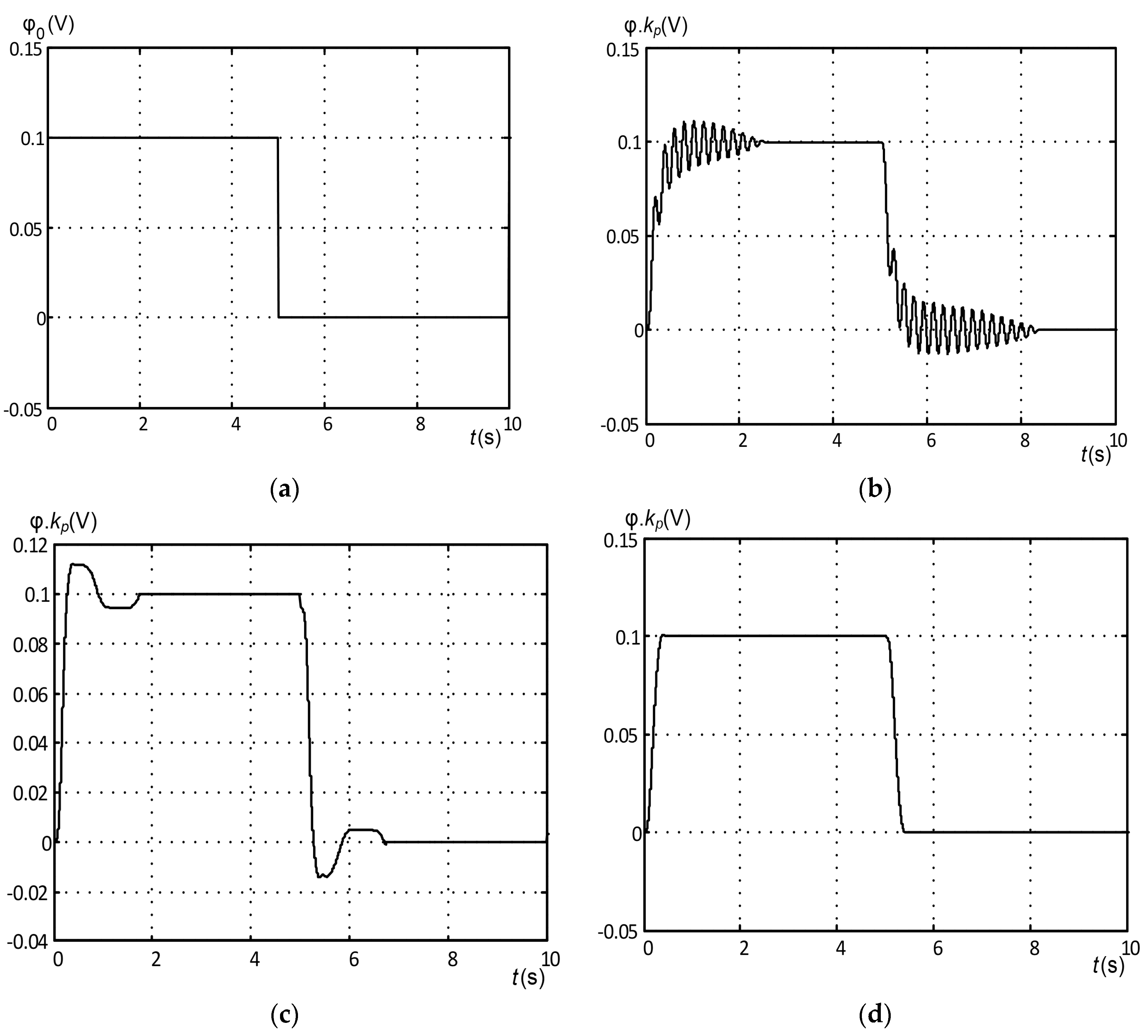
Following these parameters, our experimental results are shown in Figure 6, including the desired signal graph, the output signal graph of the control object without the controller, the output signal graph of the control object when using the modal controller, and the output signal graph of the control object when using an adaptive controller for the major functions.
Figure 6a shows the desired position signal: a square wave voltage with an amplitude of 0.1 V. It should be noted that the calculation of the angular value must take into account the transmission coefficient of the physical system (0.0412). For example, if the measured voltage value of the rotation angle is 0.1 V, then the actual value of the rotation angle is ϕ = 0.1/kp = 0.1/0.0412 = 2.43 (rad).
Figure 6b, the output signal graph of the control object without the controller, shows the initial control object’s elastic oscillations. Figure 6c shows the rotational angle graph of the second disk block when using the modal controller; the elastic vibrations have been extinguished and the rapidity of the system is improved compared to the initial control object. However, the quality of the transition is still poor because there are overshoots and two extremes, and the transition time is still long.
Figure 6d shows the rotational angle graph of the second disk block when using our adaptive controller for the major functions. The elastic vibrations have been extinguished completely, the rapidity is significantly improved compared to the initial elastic object, and it is close to the rapidity of a hard coupling. The transition process with an adaptive controller is much better than that of the non-adaptive modal controller because we had to approximate some of the parameter values used for building the linearity control object and calculating the modal controller, and in practice, those values may be different from the actual values. In contrast, our adaptive controller can control the object even when some parameter values of the control object are unspecified. Additionally, the control object is nonlinear because of the slit and friction, but these nonlinear elements are also effectively controlled by the adaptive controller. This proposed control system can be applied under different mechanical loads. In such cases, a small error may occur in the position control. However, the goal of vibration reduction is not affected, since the adaptive controller is not influenced by load momentum due to its strong impact on the inner loop (the speed loop).
5. Conclusions
The article has presented a control method based on an adaptive controller for the major functions used to control an object with elastic couplings. The object is nonlinear because of the slit and friction, but the proposed adaptive controller can control the object without knowing the parameter values. The controller’s build is optimized so that the movement quality of a drive system with elastic coupling is close to that of one with a hard coupling. The advantage of this proposed method is that the control system can operate well despite unknown object parameter values and with a nonlinear real system. Experimental results confirm the usefulness of our adaptive controller by extinguishing elastic oscillation, reducing transition time, and eliminating overshoot.
Author Contributions
Dung Tran Anh proposed the initial idea. Thang Nguyen Trong and Dung Tran Anh developed the research, analyzed the results, and wrote the article together. Thang Nguyen Trong edited and finalized the article.
Conflicts of Interest
The authors declare no conflict of interest.
References
- Hori, Y.; Sawada, H.; Chun, Y. Slow resonance ratio control for vibration suppression and disturbance rejection in torsional system. IEEE Trans. Ind. Electron. 1999, 46, 162–168. [Google Scholar] [CrossRef]
- Preitl, S.; Precup, R.E.; Stînean, A.I.; Dragos, C.A.; Radac, M.B. Control Structures for Variable Inertia Output Coupled Drives. In Proceedings of the 4th IEEE International Symposium on Logistics and Industrial Informatics (LINDI), Smolenice, Slovakia, 5–7 September 2012; pp. 179–184. [Google Scholar]
- Amann, N.; Bocker, J.; Prenner, F. Active damping of drive train oscillations for an electrically driven vehicle. IEEE/ASME Trans. Mechatron. 2004, 9, 697–700. [Google Scholar] [CrossRef]
- Boukhezzar, B.; Siguerdidjane, H. Comparison between linear and nonlinear control strategies for variable speed wind turbines. Control Eng. Pract. 2010, 18, 1357–1368. [Google Scholar] [CrossRef]
- Salman, S.K.; Teo, A.L. Windmill modeling consideration and factors influencing the stability of a grid-connected wind power-based embedded generator. IEEE Trans. Power Syst. 2003, 18, 793–802. [Google Scholar] [CrossRef]
- Chang, Y.C.; Yen, H.M. Design of a robust position feedback tracking controller for flexible-joint robots. IET Control Theory Appl. 2011, 5, 351–363. [Google Scholar] [CrossRef]
- Valenzuela, M.A.; Bentley, J.M.; Lorenz, R.D. Computer-aided controller setting procedure for paper machine drive systems. IEEE Trans. Ind. Appl. 2009, 45, 638–650. [Google Scholar] [CrossRef]
- Bahr, A.; Beineke, S. Mechanical Resonance Damping in an Industrial Servo Drive. In Proceedings of the 2007 European Conference on Power Electronics and Applications, Aalborg, Denmark, 2–5 September 2007; pp. 1–10. [Google Scholar]
- Zhang, G. Speed control of two-inertia system by PI/PID control. IEEE Trans. Ind. Electron. 2000, 47, 603–609. [Google Scholar] [CrossRef]
- Preitl, S.; Precup, R.E. An extension of tuning relations after symmetrical optimum method for PI and PID controllers. Automatica 1999, 35, 1731–1736. [Google Scholar] [CrossRef]
- Szabat, K.; Orlowska-Kowalska, T. Performance improvement of industrial drives with mechanical elasticity using nonlinear adaptive Kalman filter. IEEE Trans. Ind. Electron. 2008, 55, 1075–1084. [Google Scholar] [CrossRef]
- Dhaouadi, R.; Kubo, K.; Tobise, M. Two-degree-of-freedom robust speed controller for high-performance rolling mill drives. IEEE Trans. Ind. Appl. 1993, 29, 919–926. [Google Scholar] [CrossRef]
- Williams, R.L.; Lawrence, D.A. Linear State-Space Control Systems; John Wiley & Sons: Hoboken, NJ, USA, 2007. [Google Scholar]
- Jezernik, K.; Sabanovic, A. SMC with disturbance observer for a linear belt drive. IEEE Trans. Ind. Electron. 2007, 54, 3402–3412. [Google Scholar]
- Koronki, P.; Hashimoto, H.; Utkin, V. Direct torsion control of flexible shaft in an observer-based discrete-time sliding mode. IEEE Trans. Ind. Electron. 1998, 45, 291–296. [Google Scholar] [CrossRef]
- Erenturk, K. Nonlinear two-mass system control with sliding-mode and optimised proportional–integral derivative controller combined with a grey estimator. IET Control Theory Appl. 2008, 2, 635–642. [Google Scholar] [CrossRef]
- Xu, R.; Özgüner, Ü. Sliding mode control of a class of underactuated systems. Automatica 2008, 44, 233–241. [Google Scholar] [CrossRef]
- Brock, S.; Łuczak, D.; Nowopolski, K.; Pajchrowski, T.; Zawirski, K. Two Approaches to Speed Control for Multi-Mass System with Variable Mechanical Parameters. IEEE Trans. Ind. Electron. 2017, 64, 3338–3347. [Google Scholar] [CrossRef]
- Derugo, P.; Szabat, K. Adaptive neuro-fuzzy PID controller for nonlinear drive system. COMPEL Int. J. Comput. Math. Electr. Electron. Eng. 2015, 34, 792–807. [Google Scholar] [CrossRef]
- Graichen, K.; Zeitz, M. Feedforward control design for finite-time transition problems of nonlinear systems with input and output constraints. IEEE Trans. Autom. Control 2008, 53, 1273–1278. [Google Scholar] [CrossRef]
- Thomsen, S.; Fuchs, F.W. Flatness Based Speed Control of Drive Systems with Resonant Loads. In Proceedings of the IECON 2010—36th Annual Conference on IEEE Industrial Electronics Society, Glendale, AZ, USA, 7–10 November 2010; pp. 120–125. [Google Scholar]
- Tavakoli, M.; Taghirad, H.D.; Abrishamchian, M. Identification and robust H∞ control of the rotational/translational actuator system. Int. J. Control Autom. Syst. 2005, 3, 387–396. [Google Scholar]
- SerkieS, P. Comparison of the control methods of electrical drives with an elastic coupling allowing to limit the torsional torque amplitude. EKSPLOATACJA I NIEZAWODNOSC 2017, 19, 203. [Google Scholar] [CrossRef]
- Kang, J.K.; Sul, S.K. Vertical-vibration control of elevator using estimated car acceleration feedback compensation. IEEE Trans. Ind. Electron. 2000, 47, 91–99. [Google Scholar] [CrossRef]
- Katsura, S.; Ohnishi, K. Absolute stabilization of multimass resonant system by phase-lead compensator based on disturbance observer. IEEE Trans. Ind. Electron. 2007, 54, 3389–3396. [Google Scholar] [CrossRef]
- Katsura, S.; Matsumoto, Y.; Ohnishi, K. Modeling of force sensing and validation of disturbance observer for force control. IEEE Trans. Ind. Electron. 2007, 54, 530–538. [Google Scholar] [CrossRef]
- De Araujo, P.B.; Zanetta, L.C. Pole placement method using the system matrix transfer function and sparsity. Int. J. Electr. Power Energy Syst. 2001, 23, 173–178. [Google Scholar] [CrossRef]
- Peeters, B.; De Roeck, G. Stochastic system identification for operational modal analysis: A review. J. Dyn. Syst. Meas. Control 2001, 123, 659–667. [Google Scholar] [CrossRef]
- Duan, G.R.; Patton, R.J. Robust fault detection using Luenberger-type unknown input observers-a parametric approach. Int. J. Syst. Sci. 2001, 32, 533–540. [Google Scholar] [CrossRef]
- Hu, X.; Sun, F.; Zou, Y. Estimation of state of charge of a lithium-ion battery pack for electric vehicles using an adaptive Luenberger observer. Energies 2010, 3, 1586–1603. [Google Scholar] [CrossRef]
Figure 1.
Drive system with elastic couplings and slits.
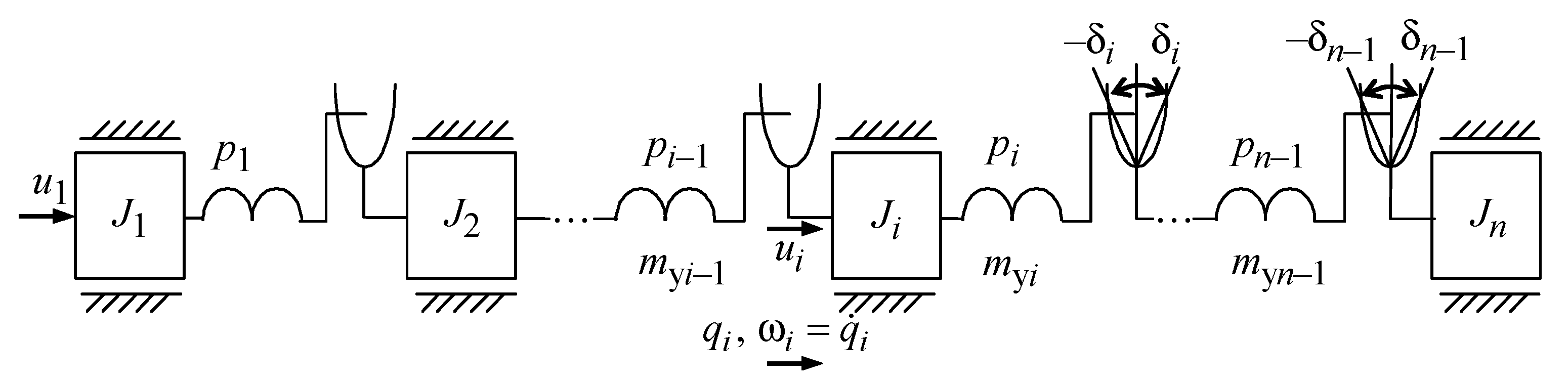
Figure 2.
Physical model of the drive system with a nonlinear elastic coupling.
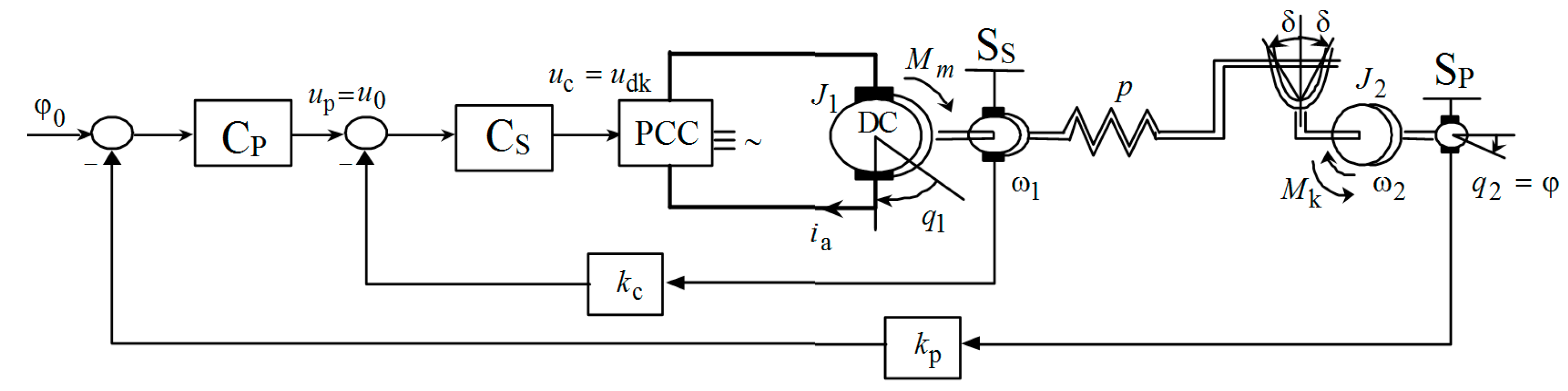
Figure 3.
The experimental system of the drive with the elastic coupling.
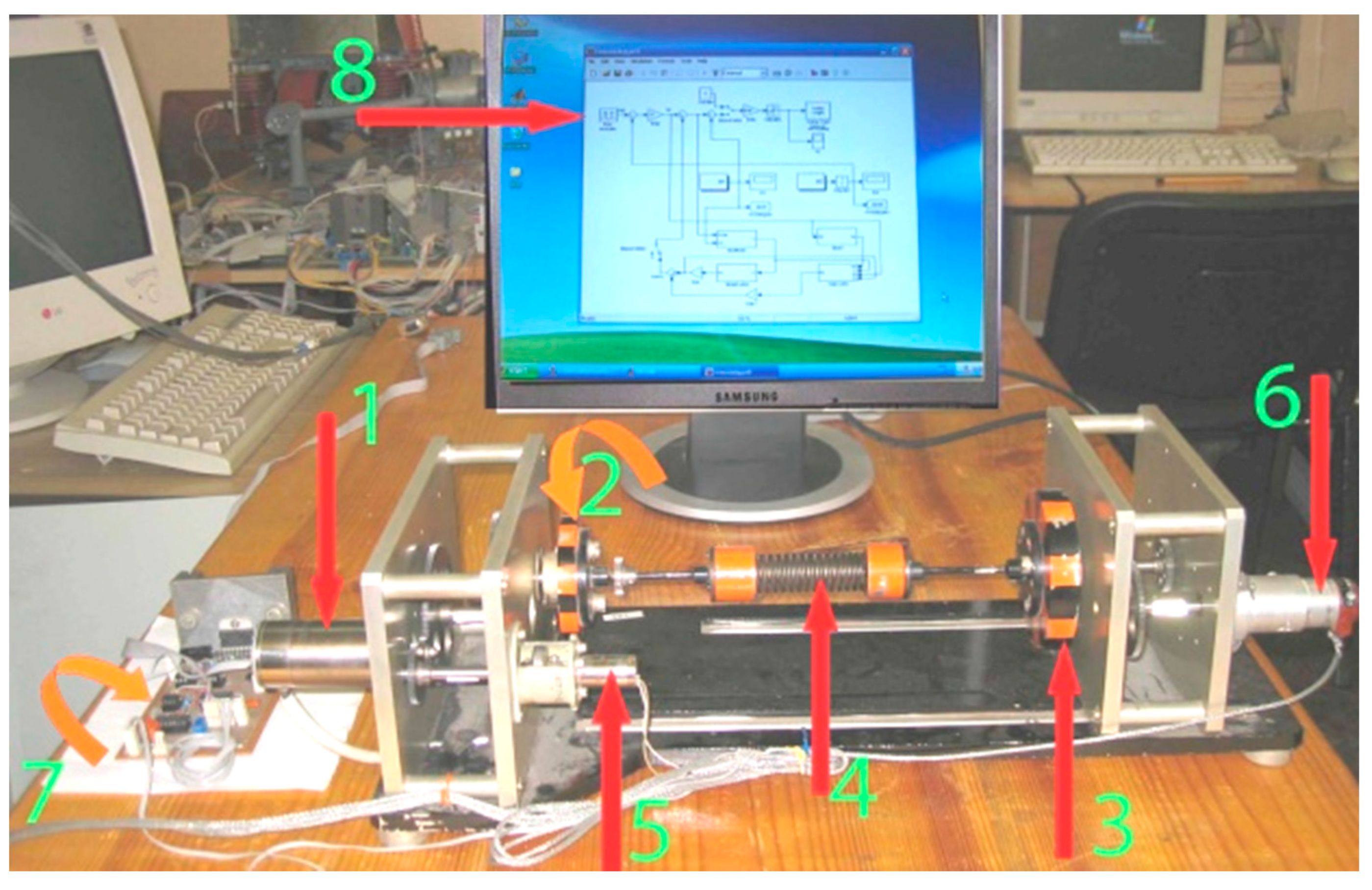
Figure 4.
The connection diagram of the system.
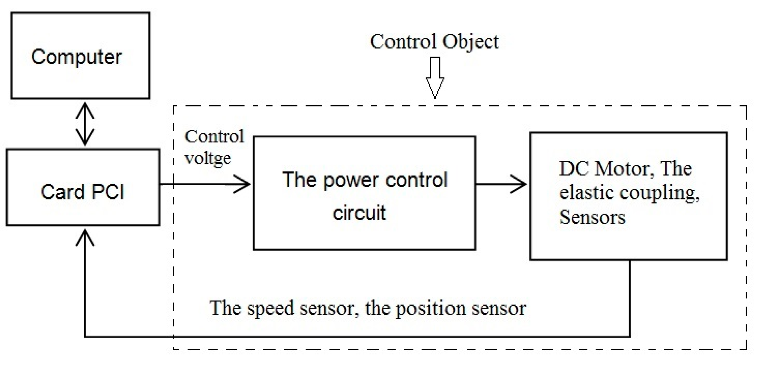
Figure 5.
The structure of the real-time controller.
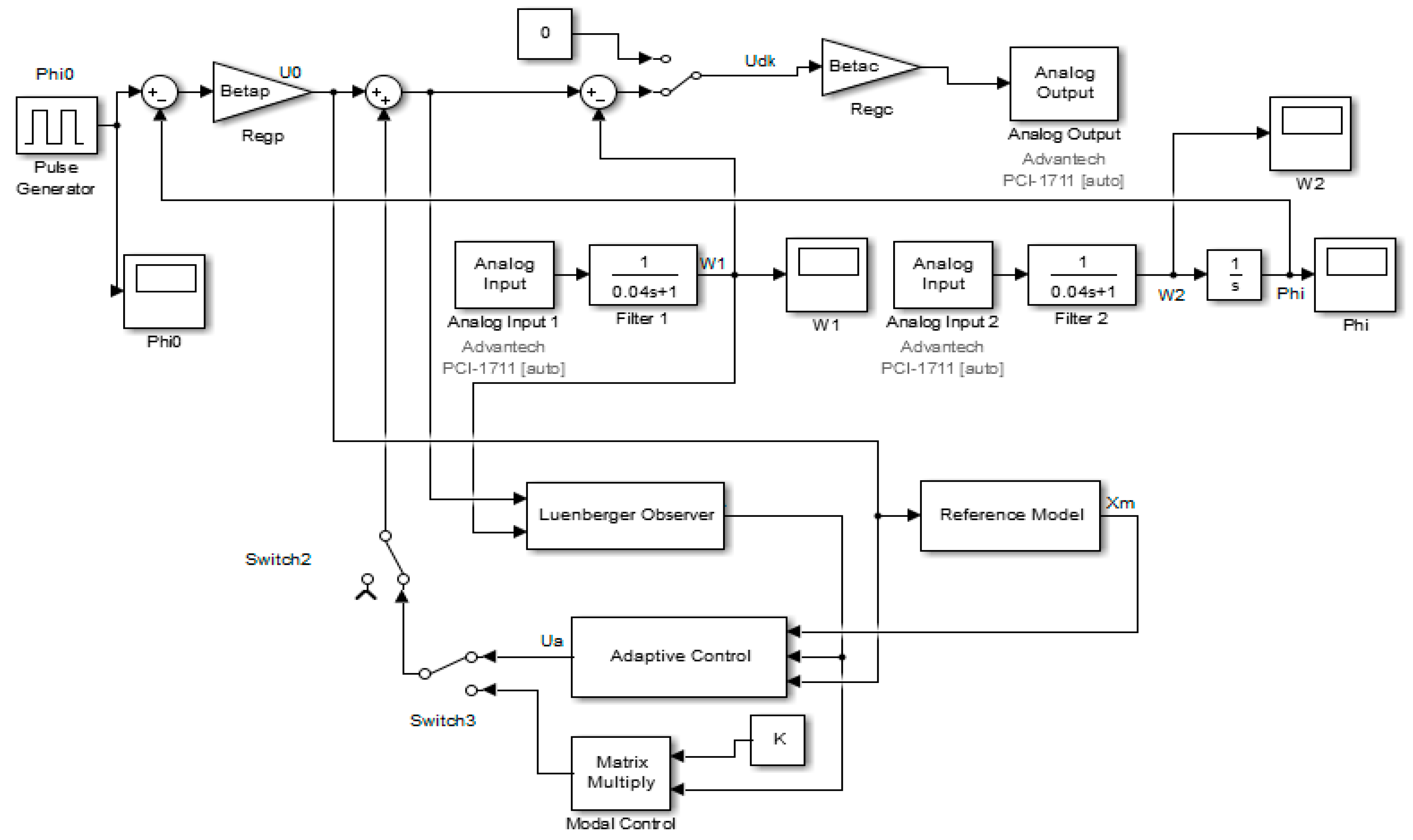
Figure 6.
The experimental results: (a) the desired position signal; (b) The output signal of the control object without the controller; (c) the output signal of the control object when using the modal controller; (d) the output signal graph of the control object when using an adaptive controller for the major functions.

© 2018 by the authors. Licensee MDPI, Basel, Switzerland. This article is an open access article distributed under the terms and conditions of the Creative Commons Attribution (CC BY) license (http://creativecommons.org/licenses/by/4.0/).
Share and Cite
MDPI and ACS Style
Tran Anh, D.; Nguyen Trong, T. Adaptive Controller of the Major Functions for Controlling a Drive System with Elastic Couplings. Energies 2018, 11, 531. https://doi.org/10.3390/en11030531
AMA Style
Tran Anh D, Nguyen Trong T. Adaptive Controller of the Major Functions for Controlling a Drive System with Elastic Couplings. Energies. 2018; 11(3):531. https://doi.org/10.3390/en11030531
Chicago/Turabian StyleTran Anh, Dung, and Thang Nguyen Trong. 2018. "Adaptive Controller of the Major Functions for Controlling a Drive System with Elastic Couplings" Energies 11, no. 3: 531. https://doi.org/10.3390/en11030531
Note that from the first issue of 2016, this journal uses article numbers instead of page numbers. See further details here.