A Reduced Order Model to Predict Transient Flows around Straight Bladed Vertical Axis Wind Turbines

Abstract

We develop a reduced order model to represent the complex flow behaviour around vertical axis wind turbines. First, we simulate vertical axis turbines using an accurate high order discontinuous Galerkin–Fourier Navier–Stokes Large Eddy Simulation solver with sliding meshes and extract flow snapshots in time. Subsequently, we construct a reduced order model based on a high order dynamic mode decomposition approach that selects modes based on flow frequency. We show that only a few modes are necessary to reconstruct the flow behaviour of the original simulation, even for blades rotating in turbulent regimes. Furthermore, we prove that an accurate reduced order model can be constructed using snapshots that do not sample one entire turbine rotation (but only a fraction of it), which reduces the cost of generating the reduced order model. Additionally, we compare the reduced order model based on the high order Navier–Stokes solver to fast 2D simulations (using a Reynolds Averaged Navier–Stokes turbulent model) to illustrate the good performance of the proposed methodology.

1. Introduction

Vertical axis wind turbines for power generation, also known as H-rotors, present complex flow phenomena associated with the blades operating in an inherently unsteady stream. These turbines consist of airfoil shaped blades that generate lift to drive a shaft, which is linked to a generator. Therefore, azimuthal changes in blade aerodynamics are unavoidable, resulting in regular time-periodic motion but also in complex flow phenomena such as stalled flows, vortex shedding and blade-vortex interactions (see [1] and references therein). The interested reader is referred to [2,3,4] for vertical axis turbines to generate wind power and to [5] for their use in urban environments.

The simulation and prediction of the temporal evolution of flows around vertical axis wind turbines is extremely difficult. This difficulty is caused, on the one hand, by the above-mentioned blade motion, which leads to unsteady flow features and dynamic effects, but also to the turbulent flow regime in which these devices operate (i.e., high Reynolds numbers). In turbulence regimes, flow structures with varying size and characteristic time scales develop. The variety of scales turns the simulation of such problems into an expensive task (in computational terms). Furthermore, the disparity of scales increases with the Reynolds number and its simulation without modelling (direct numerical simulation) becomes prohibitive at flow conditions of industrial relevance, such as when simulating wind turbines.

Turbulent flows require modelling to be simulated at an affordable cost. Modelling enables solutions on meshes that do not resolve all flow scales, but provide enough information to predict the behaviour of important flow quantities, such as the turbine blade forces or pointwise flow velocities.

Various approaches exist to avoid the expensive computational cost of resolving blade motion and turbulent flows. Examples of such approaches include modelling the blade action instead of representing their geometry in detail (e.g., actuator discs or actuator lines [3,6]) or modelling some of the small scales in turbulent flows (e.g., Reynolds Averaged Navier–Stokes (RANS) or Large Eddy Simulation (LES) approaches [7]). These models enable much faster computations at the cost of reducing fidelity to the original data. In summary, appropriate models for flows around turbines should balance fidelity (or accuracy) and computational cost.

In this work, we propose devising a high fidelity Reduced Order Model (ROM) using snapshots extracted from accurate high order simulations. This reduced order model (which is cheap to run) can be subsequently used for temporal prediction of any flow variable. The high order solver is used to simulate a vertical axis wind turbine at turbulent flow conditions with an expensive 3D high order numerical method that resolves the geometry and blade movement explicitly. Only the small scales in the turbulent flow (LES approach) are modelled in these simulations. Since these computations are expensive, the possibility of reducing the computational cost of this solver whilst maintaining the accuracy in the numerical simulations has the potential use for the wind industry. In other words, this model reproduces the near and far field of a wind turbine through the ROM fast calculations. This opens the possibility to explore complex physics at affordable costs or to model farms of turbines using ROM.

Reduced order models have become popular in representing complex physics at an affordable cost. A recent review summarises recent findings on these models [8]. Among other applications, ROM may be used as surrogates for prediction or as a replacement of costly solvers in optimisation routines. ROM have been proposed to represent horizontal axis turbine wakes, e.g., [9,10], but to the authors’ knowledge, the present work is the first to propose a ROM for vertical axis turbines.

The benefits of our ROM is that it is based on Higher Order Dynamic Mode Decomposition (HODMD) [11], a technique that extracts information of the flow dynamics of any dynamical system, thus enabling the characterisation of the system through its dominant frequencies. By selecting the most relevant frequencies of the flow system at hand (in our case, the complex flow around a Vertical Axis Turbine (VAT)), it is possible to generate a cheap ROM that can mimic the flow evolution in space and time. Although the good performance of this methodology used as a ROM has already tested in the literature [12,13], this HODMD-based ROM is novel for the computational modelling of vertical axis turbines. In summary, the developed ROM enables accurate predictions of flow states at future times, using only simulated data from early states, at a reduced computational cost.

We show that combining high order simulations with ROM enables accurate solutions (i.e., high fidelity to the original data), and outperforms cheaper 2D Navier–Stokes simulations (using a simpler turbulent model: based on a Reynolds Averaged Navier–Stokes approach). Furthermore, we show that even when the number of snapshots is small (e.g., they are collected in a time interval smaller than an entire turbine rotation), the reduced order model is capable of predicting the temporal behaviour at any time or blade azimuthal location.

The remaining of this text is organised as follows. Section 2 introduces the methodology, which includes an overview of the high order Navier–Stokes solver and details the reduced order model approach. Section 3 provides numerical results for a one bladed turbine. First, we compare the high order 3D Navier–Stokes simulations to experimental data and to a 2D low order simulation. Second, we compare the results issued from the reduced order model to the original simulated data. In a final subsection, we generate a reduced order model for a three-bladed turbine and predict the temporal behaviour at future times.

2. Methodology

In this section, we start by introducing the high order 3D Navier–Stokes solver with sliding meshes to then define the reduced order model.

2.1. High Order Numerical Solver

High order (≥3) numerical methods (e.g., spectral, discontinuous Galerkin) have seen increased popularity over the last decade [14]. These methods are characterised by low numerical errors (i.e., dispersion and diffusion) and their ability to use mesh refinement (H-refinement) and/or polynomial enrichment (P-refinement) in order to achieve accurate solutions. Polynomial enrichment provides exponential decay of the error for smooth solutions as opposed to the typical constant decay provided by the H-refinement strategy. This enables the P-refinement strategy to reach the same level of accuracy with fewer degrees of freedom.

In this work, flow solutions of the nonlinear incompressible Navier–Stokes (NS) equations, are obtained from the 3D unsteady high order (order ≥ 3) $h/p$ Discontinuous Galerkin (DG)—Fourier solver developed by the second author [15,16,17,18,19]. This high order solver provides highly accurate solutions on static and moving meshes composed of mixed triangular-quadrilateral meshes and can cope with curved boundary elements.

The solver uses a second order stiffly stable approach to discretise the NS equations in time whilst spatial discretisation is provided by the discontinuous Galerkin—Symmetric Interior Penalty formulation with modal basis functions in the x-y plane. Here, x represents the streamwise flow direction and y is the normal direction (with respect to the axis of rotation). Spatial discretisation in the z-direction (here defining the spanwise turbine length) is provided by a purely spectral method that uses Fourier series and allows computation of spanwise periodic three-dimensional flows. Since high order methods (e.g., discontinuous Galerkin and Fourier) are unable to provide enough numerical dissipation to enable under-resolved high Reynolds computations (i.e., as necessary in the Large Eddy Simulations), we have adapted the original laminar version of the solver to increase (controllably) the dissipation and enhance the stability in under-resolved simulations [19]. This dissipative formulation has minimal impact in well resolved regions and its implicit treatment does not restrict the use of relatively large time steps, thus providing an efficient stabilization mechanism for Large Eddy Simulations. The resulting solver enables 3D Large Eddy Simulation of rotating vertical axis turbines [19].

The solver has been widely validated for a variety of flows, including bluff body flows, airfoil and blade aerodynamics under static and rotating conditions [15,16,17], global instability analysis [20,21] and turbulent regimes [19]. The advantages of high order over low order methods to compute turbine flows have been discussed in [22].

2.2. A Reduced Order Model for Data Prediction

Higher Order Dynamic Mode Decomposition (HODMD) [11] is an extension of the Dynamic Mode Decomposition (DMD) approach [23], which has been recently introduced as a tool to analyze complex and noisy flows [24] or data whose spatial dimension is restricted to external conditions (i.e., hot-wire measurements or flight flutter test experiments [25]). The DMD approach extracts modes (or flow structures) from complex flows, which are ranked by frequency. This approach is different from the more classic Proper Orthogonal Decomposition [26] approach that ranks modes by energy, but cannot generally distinguish between frequencies in the flow.

HODMD approximates a set of instantaneous spatio-temporal data $\mathit{v}(\mathit{x},t_k)$, collected at time instant $t_k$ (for convenience named ${\mathit{v}}_k$) as an expansion of M DMD modes ${\mathbf{u}}_m$ that oscillate in time with frequency ${\omega }_m$, following

$${\mathit{v}}_k\simeq \sum _{m=1}^M{a}_m{\mathbf{u}}_m{e}^{({\delta }_m+i{\omega }_m)t_k}.$$

(1)

The modes are weighted with some amplitudes $a_m$ and the growth rates ${\delta }_m$ indicate the behaviour of the DMD modes in time. In transient flows, these modes may either grow or decay in time for positive or negative values of ${\delta }_m$, respectively. For permanent dynamics (attractors), the growth rates are ${\delta }_m\simeq 0$ (neither growth nor decay in time), and the DMD expansion (1) can be used, not only to reconstruct the original flow field ${\mathit{v}}_k$, but also to predict the future events if the temporal term $t_k$ is advanced in time. In other words, for a good approximation of Equation (1), it is possible to replace the temporal term $t_k$ by $t_r$, with $t_r>>t_k$. This is the main essence of using HODMD as a Reduced Order Model (ROM) [13], which is suitable for data prediction.

In order to take advantage of the model, HODMD is applied to a transitional region of a numerical simulation (or experimental data), where the number of transient modes is very large (the solution is continuously changing). The key point of this HODMD-based ROM is the way in which the permanent modes are selected to construct the expansion (1). A first alternative is to select the modes whose growth rate is close to zero based on a certain tolerance ${\epsilon }_{ext}$, so the modes considered as permanent are those satisfying the following condition $|{\delta }_m|\le {\epsilon }_{ext}$. Then, the growth rates of the selected modes are enforced to become zero, ${\delta }_m=0$, and the expansion (1) is constructed. A second alternative consists in combining HODMD with the selection criterion method of Kou and Zhang [27], known as HODMDc [12]. The modes selected by HODMDc are used to construct expansion (1). In this second case, the values of the growth rates of the modes selected are not modified. The good performance of both alternatives has been shown in the literature [12,13]. Nevertheless, for very good approximations of (1), the second method is advantageous because it can be used to predict not only permanent dynamics, but also transient stages (growing and decaying dynamics), since it takes into account the influence of the growth rates of each mode. In addition, the growth rate helps to attenuate the errors produced in the calculations of the frequencies in expansion (1), whose influence increases for temporal predictions ($t_r$). On the contrary, for very large time predictions, the decaying modes with values of ${\delta }_m<<0$ will vanish, and consequently the accuracy of the prediction might be reduced. In this article, the methodology HODMDc has been used to construct the HODMD-based ROM.

2.2.1. The Algorithm of HODMD

The HODMD algorithm is only presented briefly in this article, but the interested reader may find details in [11]. As a prior step, it is necessary to construct a snapshot matrix ${\mathit{V}}_1^K$ (of dimension $J\times K$) containing a set of K time equispaced snapshots as

$${\mathit{V}}_1^K=[{\mathit{v}}_1,{\mathit{v}}_2,\dots ,{\mathit{v}}_k,{\mathit{v}}_{k+1},\dots ,{\mathit{v}}_{K-1},{\mathit{v}}_K],$$

(2)

where each vector ${\mathit{v}}_k$ (snapshot of dimension J) is composed by the signal (e.g., flow velocity) defined at time instant $t_k$. Thus, the dimension of the snapshot matrix is $J\times K$. Then, the HODMD algorithm proceeds in two main steps:

• Dimension reduction via SVD. At this step, the spatial dimension J of the data collected is reduced to N linearly independent vectors using a singular value decomposition (SVD) [28]. By doing so, it is possible to clean the noise from the signal and to remove spatial redundancies. SVD is applied to the snapshots matrix (2):

  $${\mathit{V}}_1^K\simeq \mathit{U}\Sigma {\mathit{T}}^{\top },$$

  (3)

  where ${\mathit{U}}^T\mathit{U}={\mathit{T}}^T\mathit{T}=$ the $N\times N$ unit matrix and the diagonal of matrix $\Sigma$ contains the singular values ${\sigma }_1,\cdots ,{\sigma }_K$.
  Then, the reduced snapshots matrix of dimension $N\times K$ can be written as

  $$\begin{array}{c}{\widehat{\mathit{V}}}_1^K=\Sigma {\mathit{T}}^{\top },\mathrm{with}{\mathit{V}}_1^K=\mathit{U}{\widehat{\mathit{V}}}_1^K.\hfill \end{array}$$

  (4)
  The standard SVD-error, which determines the number of N SVD modes retained, is estimated for a certain tolerance ${\epsilon }_1$ (set by the user) as

  $$\frac{{\sigma }_{N+1}^2+\cdots +{\sigma }_K}{{\sigma }_1^2+\cdots +{\sigma }_K}\le {\epsilon }_1.$$

  (5)
  This tolerance is determined, among other factors, by the level of noise [24,29] or the level of the fluctuations of the signal [30].
• The DMD-d approximation. The reduced snapshot matrix is used to construct the following matrix according to the higher order Koopman assumption

  $${\widehat{\mathit{V}}}_{d+1}^K\simeq {\widehat{\mathit{R}}}_1{\widehat{\mathit{V}}}_1^{K-d}+{\widehat{\mathit{R}}}_2{\widehat{\mathit{V}}}_2^{K-d+1}+\dots +{\widehat{\mathit{R}}}_d{\widehat{\mathit{V}}}_d^{K-1},$$

  (6)

  where the reduced Koopman operators ${\widehat{\mathit{R}}}_k$ contain the dynamics of the system. These are collected into a single matrix $\tilde{\mathit{R}}$, called the modified Koopman matrix. The eigenvalues of the modified Koopman matrix represent the frequencies and growth/damping rates of equation (1), while the eigenvectors, combined with the SVD modes $\mathit{U}$, are used to calculate the DMD modes ${\mathit{u}}_m$ (normalized to exhibit unit norm). Finally, the amplitudes related to each mode are calculated by least squares fitting of the expansion (1). In HODMD, the most relevant M DMD modes are retained as function of their amplitudes, depending on a second tolerance ${\epsilon }_2$ (set by the user), where

  $$a_m/a_1<{\epsilon }_2,m=1,\dots ,M.$$

  (7)
  The selection of the modes will be replaced by the selection criterion method [27] presented below for the construction of the HODMD-based ROM (expansion (1)).
  Once the DMD expansion (1) is approximated, the root mean square error (RMSE) is used to quantify the difference between the original data and the approximated solution (1), following

  $$RMSE\sim \frac{\left|\right|{\mathit{V}}_{original}-{\mathit{V}}_{DMD}{\left|\right|}_F}{\left|\right|{\mathit{V}}_{original}{\left|\right|}_F},$$

  (8)

  where $\left|\right|·{\left|\right|}_F$ represents the Frobenius norm.

Finally, it should be noticed that when $d=1$ in (6), the HODMD algorithm is similar to original DMD algorithm [23], and, consequently, the results provided by both algorithms are the same. However, this is not the case when $d>1$. The parameter d is set by the user, through a calibration phase based on the robustness of the results (for various ${\epsilon }_1$, ${\epsilon }_2$, $\Delta t$ and various d). The final results should become independent of these parameters or, in other words, need to be robust to small variations of these parameters [24].

2.2.2. Criterion Selection Method

A new criterion selection method has been recently introduced by Kou and Zhang to select the most relevant DMD modes to construct the DMD expansion (1). When the criterion is combined with HODMD, the method is called HODMDc [12]. The criterion selection method considers the initial condition and the temporal evolution of each DMD mode, and is based on the parametrised DMD approach [31] (i.e., determining the amplitude of each DMD mode as a time dependent coefficient). Thus, it is possible to write the DMD expansion (1) as

$${\mathit{v}}_k\simeq \sum _{m=1}^M{b}_m\left(t_k\right){\widehat{\mathbf{u}}}_m,$$

(9)

where $b_m\left(t_k\right)$ is the temporal coefficient, which changes with time as flow evolves, and ${\widehat{\mathbf{u}}}_m$ is the DMD mode normalized with the square of the Frobenius norm. Using a more general description of Equation (9), it is possible to evaluate the contribution of each mode to the complete data set, by means of its temporal coefficient. Integrating in time the term $|b_m\left(t_k\right)|$, it is possible to calculate the energy index of each mode $I_m$ as

$$I_m=\int |b_m\left(t\right)|dt\simeq \sum _{k=1}^K\left|b_m\left(t_k\right)\right|dt,$$

(10)

which yields the following expression (when applied to expansion (1)),

$$I_m=\sum _{k=1}^K|a_m{e}^{({\delta }_m+i{\omega }_m)}\left|\right||{\mathbf{u}}_m{\left|\right|}_F^2\times \Delta t,$$

(11)

representing $\left|\right|·{\left|\right|}_F^2$ the square of the Frobenius norm. Once that the terms of the DMD expansion (1) are calculated using HODMD, each DMD mode is ranked according to the parameter $I_m$. Then, the M modes with higher value of $I_m$ are used to construct Equation (1). The number of M DMD modes retained can be set either using a specific tolerance ${\epsilon }_2$ as in Equation (7) or giving the number of retained mode pairs. In the following sections, M will be varied to construct several ROMs and the resulting ROM based predictions compared.

3. Numerical Results

3.1. Numerical Simulations for a One Bladed Vertical Axis Turbines

A particular challenge when simulating cross-flow turbines is the relatively high Reynolds number at which these devices operate. Flow regimes for wind turbines are generally turbulent. Numerous studies have computed vertical axis turbines using numerical low order methods, e.g., Ref. [32,33,34,35,36,37] and only very recently Ferrer [19] has provided results for vertical axis turbines using high order solvers and moving meshes.

In this section, we perform numerical simulations for a one bladed turbine. We compare 3D simulated results issued from the high order Navier–Stokes solver with experimental data and also to fast 2D simulations computed using the commercial finite volume solver Ansys-Fluent-16.2 [38] This solver is selected to simulate unsteady Reynolds Average (uRANS) Navier–Stokes solutions using a k-omega Shear Stress Transport (SST) turbulence model. These simulations will provide an idea of what to expect from cheap numerical simulations or simple models, so we can assess in upcoming sections the validity of our new reduced order model based on HODMD.

Both high order and low order solvers use sliding meshes and rotate the mesh as time evolves. The high order solver computes 3D simulations (as required by LES type turbulent models) whilst Fluent (using uRANS) allows cheaper 2D simulations. The former involves more expensive simulations, but these are typically more accurate. Numerical details of both solvers are summarised in

Table 1. Numerical details of the Navier–Stokes computations for a one bladed rotating turbine. The out-of-plane length (marked *) for the high order mesh is discretised using 64 Fourier planes. The high order mesh (marked **) includes the number of elements and the polynomial order P = 3 and 64 Fourier planes for the 3D mesh. For the low order model (marked ***), almost identical results were obtained with a finer mesh of 31,584 elements.

	High Order Solver	Low Order Fluent
Blade/Mesh movement	Sliding mesh	Sliding mesh
Numerical scheme	3D DG-Fourier	2D Finite Volume
Out-of-plane length	0.5 m *	0 m
Turbulence model	Large Eddy Simulation	k-omega SST (uRANS)
Numerical details	polynomial order P = 3	Second order Upwind
Order of accuracy	3	2
Mesh size	1.1 millions **	7896 ***
Time advancement	2nd order semi-implicit	1st order implicit
Time step	0.001 s	0.2 s

. We show the meshes and a snapshot of the numerical solutions for both solvers in Figure 1. The turbine has a diameter of radius $R=4$ m (distance form the center of rotation (x, y) = (0, 0) to the airfoil quarter chord. This means that the position of the blades lie within the interval $x\in$ [−4 m, 4 m] and $y\in$ [−4 m, 4 m].

Experimental and numerical conditions are detailed in

Table 2. Vertical axis turbine conditions. All in international metric system. $TSR=\omega D/2U$ denotes the tip-speed ratio, $R{e}_c=\frac{c}{\nu }\sqrt{{(\omega D/2)}^2+U^2}$ is the Reynolds number based on the chord and rotating speed whilst $R{e}_D=\frac{DU}{\nu }$ is based on the turbine diameter and free stream velocity .

	Blade	Turb.	Length	Stream	Rot.	Tip Speed	Kin.	Reynolds
	Chord	Diameter	Ratio	Vel.	Speed	Ratio	Visc
Symbol	c	D	$c/D$	U	$\omega$	$TSR$	$\nu$	$R{e}_c$	$R{e}_D$
Units	m	m	-	m/s	rad/s	-	m2/s	-	-
Oler et al. [39]	0.1524	1.22	0.125	0.091	0.749	5	$0.1\times {10}^{-5}$	$6.83\times {10}^4$	$1.07\times {10}^5$
Simulations	1.0	8.0	0.125	0.088	0.11	5	$5.0\times {10}^{-5}$	$0.90\times {10}^4$	$0.14\times {10}^5$

for the one bladed turbine, whose blade geometry is characterised by a NACA0015 airfoil. We have maintained the main characteristic numbers $c/D$, the tip speed ratio ($TSR=\frac{\omega D}{2U}$).

We compare the simulated results to experimental tests [39] for the normal non-dimensional blade forces $C_N=\frac{2F_i}{\rho c{U}^2}$, and $\rho$ represents the fluid density, for a rotating one bladed vertical axis turbine. Figure 2a compares instantaneous values for the 3D high order DG method to averaged experimental values for four revolutions. We observe comparatively good agreement between 3D high order DG computations (black line) and experiments (orange and blue lines). The experimental data by Oler et al. [39] includes strain gauge data and pressure data. Whilst the former was reported to be accurate by Oler et al., the latter was obtained by integration of pressure force coefficients (using only five probes) and has been reported to “contain a reasonable amount of error”. Despite the errors, we have included the pressure data to quantify possible experimental errors and to show that the high order simulations are close, in comparative terms, to the gauge data. Additionally, let us note that the experimental forces where filtered using a low pass filter (with frequency 0.6 Hz) whilst our simulations are depicted for a sampling frequency of 1000 Hz, which explains the nosier data of the simulations when compared to the experimental forces.

Figure 2b compares the low order 2D Fluent solution to the experimental values. We observe good overall agreement but less accuracy than when the high order solver is used.

Previous publications [39,40,41,42,43] have compared forces for cheap computational and analytical models to the experiments of Oler et al. [39] but have showed generally higher discrepancies that our computations. Additionally, these publications have reported non-negligible errors in the experimental measurements for the tangential forces. Consequently, we have preferred to include only the normal forces, which are experimentally accurate and sufficient to show the differences in accuracy between our high and low order simulations.

Returning to the streamwise-velocity snapshots shown in Figure 1a.2,b.2, we observe a more complex flow with multiple vortices emanating from the trailing edge, when using the high order LES approach and a much smoother flow (with fewer flow details) when using the low order solver with uRANS turbulence. Both the time evolution of the forces and the instantaneous flows suggest that a high order solver with an LES turbulent closure is more accurate than the low order uRANS model. The computational time for the low order model is orders of magnitude lower than when using the high order method, which is attributed the the smaller mesh (2D vs. 3D) and the higher time step enabled by the simpler method and coarser mesh (see Table 2).

Finally, we compare velocity components: streamwise ($u_x$) and normal ($u_y$), on two horizontal lines at $y=-2$ m and $y=-4$ m for a fixed simulation time in Figure 3. At this instant in time, the blade is at an azimuthal angle of ${153}^{°}$ (measured from the 12:00 a.m. position and rotating anti-clockwise), such that the first line ($y=-2$ m) is at the back of blade trailing edge, whilst the second line ($y=-4$ m) is at the front of the rotating blade. Figure 3 shows that the low order Navier–Stokes solver that uses an uRANS turbulent model provides similar trends that the high order LES simulation, but does not capture all details. In the next sections, we will develop a reduced order model that can capture most of the complex flow physics present in the high order simulation at an affordable computational cost.

3.2. Reduced Order Model for a One Bladed Vertical Axis Turbine

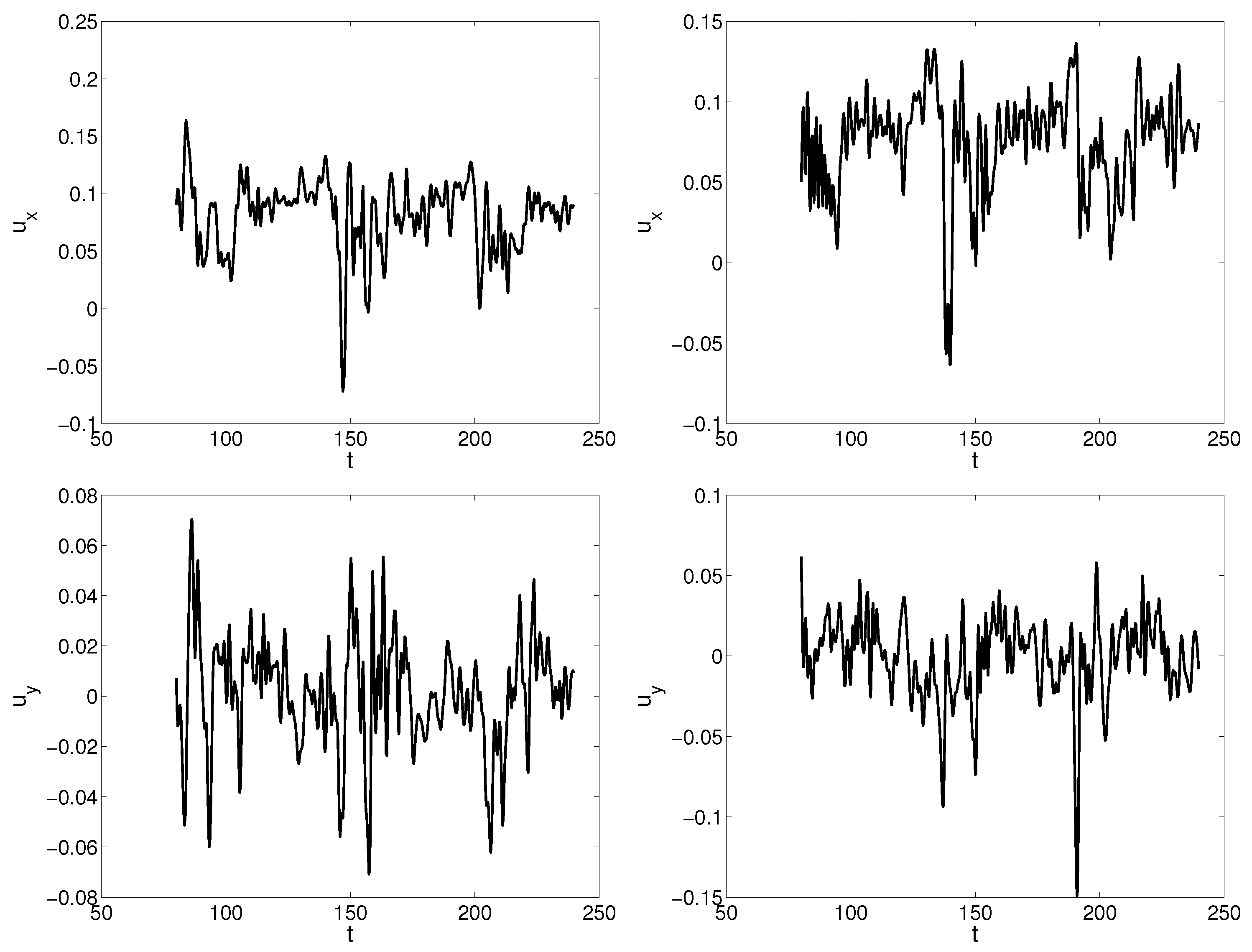
We use the result from the 3D high order numerical simulations for the one bladed turbine, and construct an HODMD-based ROM using 196 snapshots equispaced in time, with $\Delta t=0.3$ s. Two-dimensional snapshots are extracted from the 3D simulation. These snapshots are collected after one and a half blade revolutions ($t=80.01$ s), in order to avoid spurious and transient artifacts of the numerical solution. Consequently, the snapshots are collected during the time interval 80.01 s $\le t\le 138.51$ s (58.5 s representing $58.5\times \omega \times \frac{{180}^{°}}{\pi }\simeq {368}^{°}$ of rotation). Let us remember that a complete rotation of the wind turbine (${360}^{°}$) is represented by $\frac{2\pi }{\omega }\simeq 57.12$ s time units (with rotation velocity $\omega =0.11$ rad/s). Figure 4 shows the temporal evolution, which includes the temporal interval retained for this analysis, of two representative points located near the blades rotation region: $P(x_1,y_1)=(0,-4)$ and $P(x_2,y_2)=(2.8,-2)$ with coordinates in meters. As seen in Figure 4, the flow complexity is very large due to the high level of fluctuations (since the flow is turbulent).

After some calibration, based on the robustness (similar solutions for various type of calculations) of the results [24,29], the parameters used for the HODMD analysis are $5\le d\le 10$, ${\epsilon }_1={\epsilon }_2={10}^{-3}$. It is remarkable that, although the flow is highly complex and the analysis is carried out in an unsteady regime of a numerical simulation (only ∼1 blade revolution is analysed), which limits the values of d used for the analysis [29], the results are robust. Nevertheless, the solution obtained would improve when using a larger value for d, if more snapshots are retained. The reason is that the HODMD expansion, characterized by d reduces data uncertainty [24] and helps removing the transient modes, which are treated by the method as noise [13]). Regarding the tolerances, Figure 4 shows that there are small variations of velocity, of order ${10}^{-2}$ (velocity fluctuations), which represent variations of 10% with respect the mean velocity. So, the tolerances ${\epsilon }_1$ and ${\epsilon }_2$ (see Section 2.2) should be below ${10}^{-2}$ to reproduce accurately these fluctuations. In this case, we have set such tolerances to one order of magnitude below to remain conservative. Note that values below ${10}^{-3}$ could introduce spurious artifacts in the reduced order model, due to the large complexity of this flow (which is fully turbulent) and should be avoided.

The data complexity and the unfavorable conditions to construct a DMD-based ROM (unsteady turbulent flow and transient data, small time interval to collect the data) suggest that the best option for this case is to combine HODMD with the criterion selection method (HODMDc) that will identify the most relevant modes that will be used to generate the ROM.

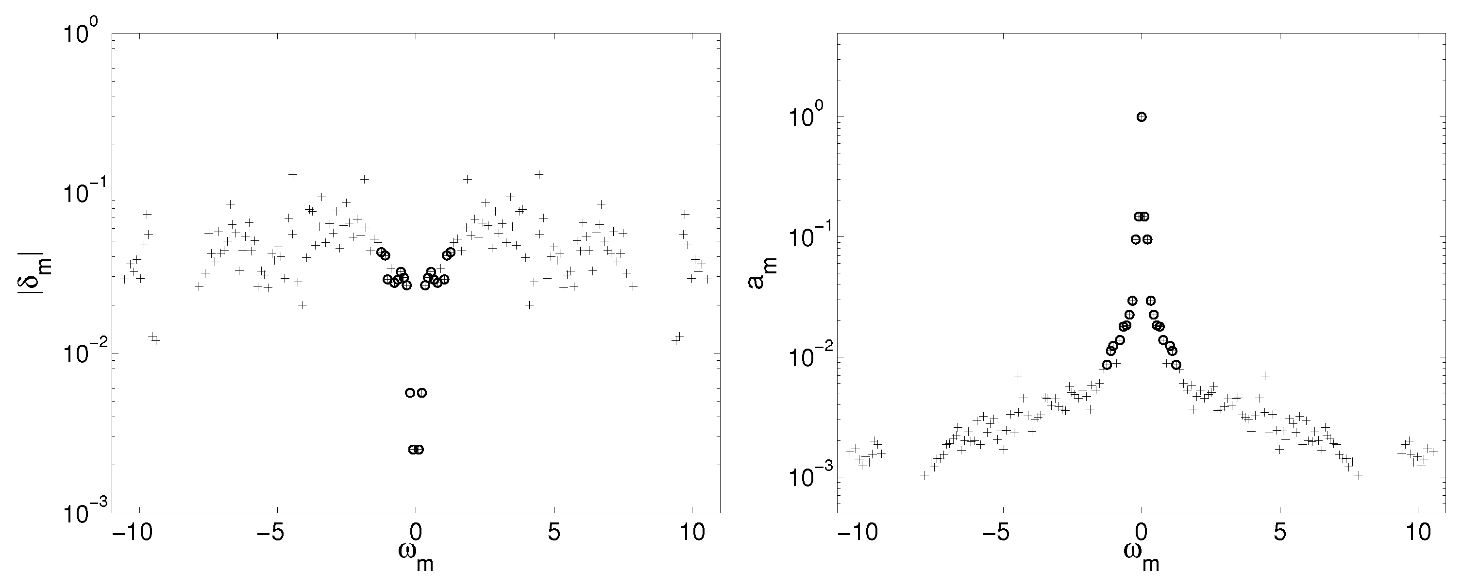
Figure 5 shows the growth rates and the amplitudes as function of their corresponding frequencies in the HODMD analysis. As seen, the numerical simulation is still under a transient stage, since the order of magnitude of the growth rates of the DMD modes is defined in the interval (10${}^{-2}$ s, 10${}^{-1}$ s) (transient solution). The method identifies 65 frequencies. HODMDc has been applied to find the most relevant frequencies for the ROM. The prediction of the results has been carried out retaining several number of modes: $M=3$ in a first case, $M=5$ and $M=21$. These frequencies are written, for clarity, in

Table 3. Frequencies selected by HODMDc (in rad/s) presented in Figure 5.

m	${\mathit{\delta }}_{\mathit{m}}$	${\mathit{\omega }}_{\mathit{m}}$	${\mathit{a}}_{\mathit{m}}$	M
1	−9.5158 × ${10}^{-3}$	1.0418 × ${10}^{-1}$	8.3676 × ${10}^{-2}$	3
2	−1.3190 × ${10}^{-2}$	2.0196 × ${10}^{-1}$	4.3080 × ${10}^{-2}$	5
3	−5.5556 × ${10}^{-3}$	4.2243 × ${10}^{-1}$	4.5354 × ${10}^{-2}$	7
4	8.5601 × ${10}^{-2}$	1.0403 × 10	1.1669 × 10	9
5	9.8704 × ${10}^{-2}$	8.6673	2.1948 × 10	11
6	8.7053 × ${10}^{-2}$	1.0250 × 10	9.6744	13
7	−2.8024 × ${10}^{-2}$	3.0565 × ${10}^{-1}$	9.0310 × ${10}^{-3}$	15
8	4.7800 × ${10}^{-2}$	4.5260	6.1397 × ${10}^{-1}$	17
9	−1.9750 × ${10}^{-2}$	5.2824 × ${10}^{-1}$	1.2018 × ${10}^{-2}$	19
10	8.5236 × ${10}^{-2}$	8.8956	6.9477	21

, including their corresponding amplitudes and growth rates. There is a single mode with null frequency that represents the mean flow. This mode is found in all the analyses, and will not be mentioned again for the sake of brevity. The remaining modes are represented by a complex number (representing the frequency) and its complex conjugate. In other words, when the number of modes retained for the ROM construction is for example $M=3$, the DMD expansion (1) will include 3 modes, one related to the mean flow (zero frequency), one related to the dominant frequency ${\omega }_1$ and its complex conjugate $-{\omega }_1$.

As seen in the results, HODMDc always captures the mode with highest amplitude, and frequency ${\omega }_1\simeq 0.1$ rad/s (when $M\ge 3$). This frequency represents the frequency of rotation of the wind turbine blade ($\omega \simeq 0.11$ rad/s). The errors in the calculations of this frequency are attributed to the reduced temporal interval in which the snapshots are collected. Despite this, the method gives a reasonable good approximation of the fundamental frequency. When the number of modes retained is $M=5$, the method also captures the harmonic of the fundamental frequency ${\omega }_2\simeq 0.2$ rad/s. Finally, for values of $M>5$, the method captures some harmonics of the fundamental frequency and some high amplitude modes with $a_m>1$. On the one hand, these very high amplitude modes are related to the fluctuations of the wind turbine. Since the value of their growth rate is positive and ∼10${}^{-1}$, the influence of these high amplitude modes will grow in time, meaning that, for very large temporal approximations, these modes should be either omitted (as in the ROM proposed in [13]) or re-calculated at different time instants, but this is far from the scope of this article. On the other hand, although the flow is fully turbulent, it is dominated by a periodic behaviour (geometrical rotation), which is apparent by the modes retained by HODMDc. It is remarkable that the third mode captured by HODMDc is the fourth harmonic of ${\omega }_1$, ${\omega }_m\simeq 4.2·{10}^{-1}$ rad/s, instead of the third harmonic ∼3$·{10}^{-1}$ rad/s, which is selected in 7th place ($m=7$).

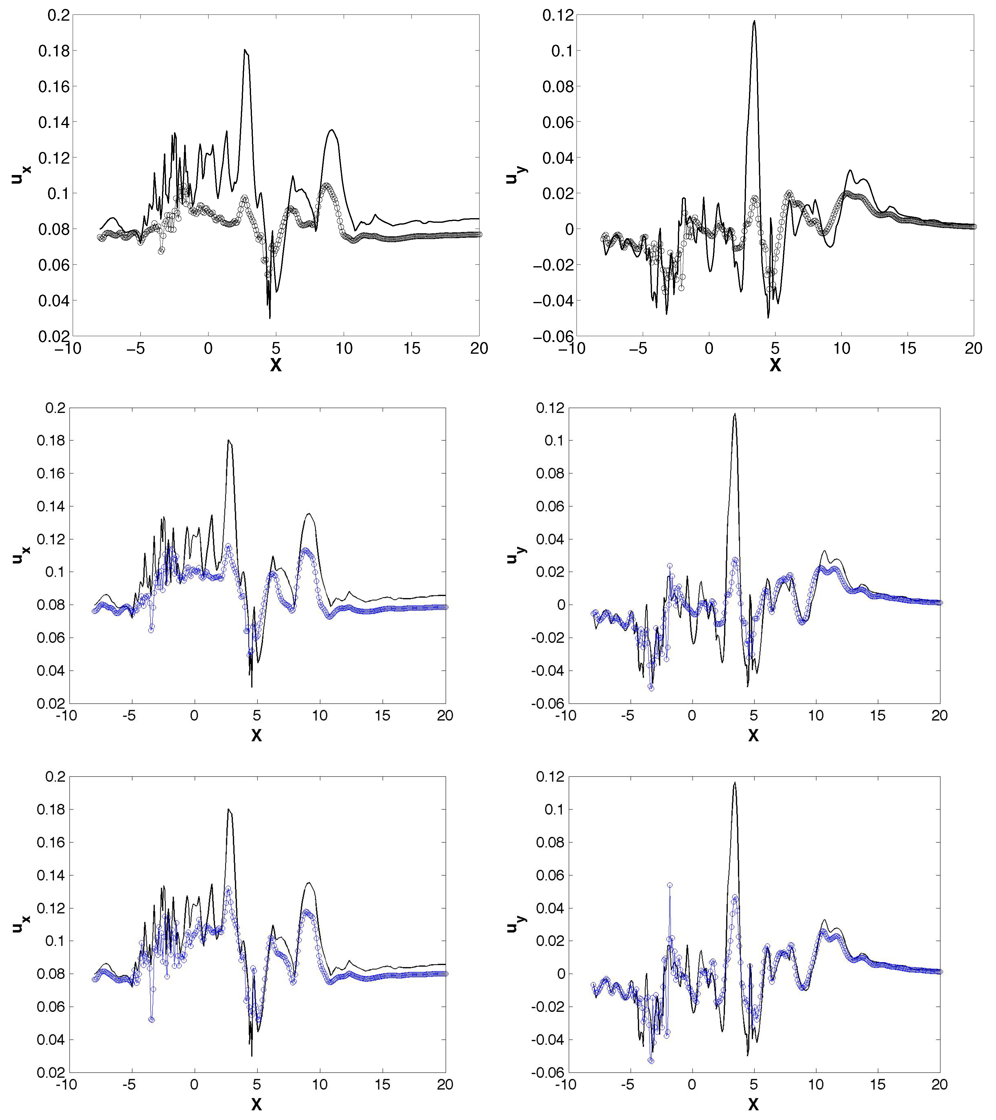
Once the HODMDc has selected the relevant DMD modes, three HODMD-based ROMs are constructed retaining $M=3$, 5 and 21 DMD modes and the solution is extrapolated in time ∼160 s time units (the following ∼4 rotations of the wind turbine). In other words, the temporal term of the DMD expansion (1) is set to $t=240$ s. Figure 6 shows the original (simulated with the high order DG method) and the predicted instantaneous flow field at time 240 s for the three ROMs constructed. As seen, the results agree favourably to the original data, predicting the regions of larger influence of the turbine blades ($y=-2$ m). The solution is smoother when the number of modes retained is smaller (and somewhat similar to the low order uRANS simulation shown in Section 3.1), but the fidelity of the model improves significantly when the number of modes is increased. However, it is interesting to note that, using only 3 DMD modes ($M=3$), it is possible to represent the main structures of the wind turbine. The RMS error of these predictions is ∼28% , ∼25% and ∼23% for $M=3$, 5 and 21, respectively. These errors appear large, having seen the good qualitative agreement of the figures.

In order to understand these errors, Figure 7 and Figure 8 compare the original and approximated spatial evolution of the solution at constant time 240 s and two representative horizontal lines at $y=-4$ m and $y=-2$ m (at a fixed instant in time). The figures show that the three ROMs predict the mean flow field correctly. The predictions with the model with five modes is better than the one of three modes. The model that uses 21 modes is able to approximate some of the high frequency peaks that are related to small scales fluctuations, and related to the modes with very high amplitude. When removing these peaks (i.e., when $x>5$ m), the HODMD model predicts the solution with a global RMS error smaller than 15%, 13% and 10%, in the models constructed with 3, 5 and 21 modes, respectively. These results reflect that the optimal model is the one retaining five modes, not only because the growth rates of the modes are negative (avoiding that the results diverge at large times), but also because the error for $M=5$ is similar to the error obtained with $M=21$ modes, proving that including more modes does not result necessarily in a more accurate model.

3.3. Extensions for Three Bladed Vertical Axis Turbine

In the previous section, we developed and validated a ROM model for a one bladed turbine using snapshots extracted from a 3D high order simulation. In this section, we proceed similarly and generate a ROM model for a three-bladed turbine. The motivation to study this new geometry is three-fold. First, typically, a vertical axis wind turbine has three blades. Second, three blades tend to generate more complex flows (e.g., more vortex-blade interactions [1], and third, the potential for computational cost savings are greater since three bladed turbines require typically more mesh elements. Furthermore, we will generate the ROM using snapshots exacted during less than one full revolution and show that this is enough to represent the complete turbine behaviour.

The 3D mesh for the high order DG-Fourier solver uses 3676 elements, with polynomial order P = 3 and 64 Fourier planes, given a total number of degrees of freedom of 2.35 millions (2.14 times more that for the one bladed turbine).

As in the previous section, we extract 2D snapshots from the 3D high order simulations and construct an HODMD-based ROM using 196 snapshots equispaced in time. These snapshots have been taken in the time interval $44.4$ s $\le t\le$ 102.416 s ($58.016$ s, representing ≃$365.65°$), equispaced in time with $\Delta t=0.296$ s. With the aim of reducing the computational cost and increasing the efficiency of the ROM methodology, we shift the window for analysis to an an earlier time (than in the previous case). Figure 9 shows the temporal evolution in the interval analyzed of two representative points collected in the blades area of the wind turbine, $P(x_1,y_1)=(0,-4)$ and $P(x_2,y_2)=(2\sqrt{2},2\sqrt{2})$ meters. As seen, the flow complexity is large due to the velocity fluctuations. In addition, the figure shows that the flow is still evolving in time and consequently the numerical simulation has not reached a periodic state. This will serve to prove the good performance of the method if the snapshots collected do not cover an entire rotation of the turbine blade (but only $270°$). This shortened sampling interval increases the possibility of finding spurious artifacts in the analysis of the simulations, but we show that the proposed method can handle these difficulties. Once the ROM is generated, we use it to predict a solution evolved in time until ∼160 s time units; i.e., the temporal term of expansion (1) is set for this prediction at $t=202.8$ s.

Similarly to the previous case, the parameters used in this analysis are $5\le d\le 10$ and the tolerances ${\epsilon }_1={\epsilon }_1={10}^{-3}$. Figure 10 shows the frequencies as function of their amplitudes and growth rates obtained in the analysis. The HODMD method produces 151 modes.

Table 4. Frequencies selected by HODMDc (in rad/s) presented in Figure 10.

m	${\mathit{\delta }}_{\mathit{m}}$	${\mathit{\omega }}_{\mathit{m}}$	${\mathit{a}}_{\mathit{m}}$	M
1	−2.4974 × ${10}^{-3}$	1.0372 × ${10}^{-1}$	1.4785 × ${10}^{-1}$	3
2	−5.6401 × ${10}^{-3}$	2.1195 × ${10}^{-1}$	9.5278 × ${10}^{-2}$	5
3	−2.6524 × ${10}^{-2}$	3.3103 × ${10}^{-1}$	2.9438 × ${10}^{-2}$	7
4	−2.9580 × ${10}^{-2}$	4.3577 × ${10}^{-1}$	2.2503 × ${10}^{-2}$	9
5	−3.2188 × ${10}^{-2}$	5.4754 × ${10}^{-1}$	1.8342 × ${10}^{-2}$	11
6	−2.8720 × ${10}^{-2}$	6.5329 × ${10}^{-1}$	1.7896 × ${10}^{-2}$	13
7	−2.7517 × ${10}^{-2}$	7.8174 × ${10}^{-1}$	1.3842 × ${10}^{-2}$	15
8	−2.8857 × ${10}^{-2}$	1.0277	1.2363 × ${10}^{-2}$	17
9	−4.0700 × ${10}^{-2}$	1.1119	1.1227 × ${10}^{-2}$	19
10	−4.2714 × ${10}^{-2}$	1.2517	8.6121 × ${10}^{-3}$	21

shows the frequencies, amplitudes and growth rates obtained using HODMDc and retaining 3, 5 and 21 modes (the mode corresponding the mean flow is included in all cases). As for the one bladed turbine, the first frequency retained by HODMDc is the one with highest amplitude ${\omega }_1\simeq 0.1$ rad/s that represents the frequency of rotation of the turbine blade ($\omega \simeq 0.11$ rad/s). The following six frequencies are harmonics of this fundamental frequency and the remaining three frequencies are also high order harmonics of ${\omega }_1$. In contrast to the previous case, the number of harmonics of ${\omega }_1$ retained by this ROM is larger, representing the major influence of the three blades in the periodic behaviour of the flow. This is also reflected in the amplitude of the DMD modes, since the modes retained by HODMDc correspond to the ones with the highest amplitude. The same analysis has been carried out in different planes of the three-dimensional computational domain to check that the results are very similar and independent of the out-of-plane location (these results are not shown for the sake of brevity).

Figure 11 compares the instantaneous original (high order 3D simulation) and predicted flow fields for the three ROMs constructed with $M=3$, 5 and 21 DMD modes, at time $202.8$ s. As seen, these predictions are in good agreement with the original solution. As expected, small flow structures are better represented when the number of modes retained is larger. However, it is interesting to note that the overall flow structure defining the turbine blade movement can be represented with only three modes. As in the previous case, the RMS error is high in the three cases, being ∼40% (in all the cases). Figure 12 and Figure 13 show that, as already explained, the model cannot predict the peak values of the velocity fluctuations, but that when these peaks are removed (i.e., when $x>5$ m), the model predicts the original solution with high accuracy (RMS error is ∼15–20%).

Finally, we challenge the HODMD-based ROM by decreasing the number of samples used to construct the ROM. We perform the same analysis but use only 145 snapshots equispaced in time, with $\Delta t=0.296$ s collected in the time interval 25.604 s $\le t\le$ 68.524 s ($42.92$ s time units, representing $42.9\times \omega \times \frac{180°}{\pi }\simeq 270°$). Now, the data collected do not represent a complete rotation, making this problem even more challenging than the previous one. In addition, the data set has been taken earlier than before (almost half a rotation earlier). In the first part of the simulation, the data are unstable and are neglected as fully transient (a part of the initialisation of the simulation). This means that these snapshots cannot be used to represent any event in the future (attractor) of the numerical simulation. The parameters used for the HODMD analysis are $1\le d\le 5$, ${\epsilon }_1={\epsilon }_2={10}^{-3}$ (the interval defined for d has decreased with the number of snapshots).

Figure 14 shows the growth rates and the amplitudes as a function of their corresponding frequencies in the HODMD analysis. The method identifies 134 frequencies.

Table 5. Frequencies selected by HODMDc (in rad/s) presented in Figure 14.

m	${\mathit{\delta }}_{\mathit{m}}$	${\mathit{\omega }}_{\mathit{m}}$	${\mathit{a}}_{\mathit{m}}$	M
1	−3.0199 × ${10}^{-2}$	1.3516 × ${10}^{-1}$	8.5508 × ${10}^{-2}$	3
2	−4.0940 × ${10}^{-2}$	2.6042 × ${10}^{-1}$	4.9633 × ${10}^{-2}$	5
3	−3.0227 × ${10}^{-2}$	4.2156 × ${10}^{-1}$	4.3403 × ${10}^{-2}$	7
4	−4.0559 × ${10}^{-2}$	5.9441 × ${10}^{-1}$	3.7762 × ${10}^{-2}$	9
5	−5.0647 × ${10}^{-2}$	8.5848 × ${10}^{-1}$	3.0700 × ${10}^{-2}$	11
6	−9.1483 × ${10}^{-2}$	1.4785	2.2538 × ${10}^{-2}$	13
7	−3.8967 × ${10}^{-2}$	1.1690	3.1258 × ${10}^{-2}$	15
8	−1.0826 × ${10}^{-1}$	1.5864	1.8197 × ${10}^{-2}$	17
9	−6.2864 × ${10}^{-2}$	1.3355	2.3832 × ${10}^{-2}$	19
10	−7.8737 × ${10}^{-2}$	7.2259 × ${10}^{-1}$	2.0244 × ${10}^{-2}$	21

shows the frequencies, amplitudes and growth rates obtained using HODMDc retaining $M=3$, 5 and 21 modes. Again, the first frequency retained by HODMDc is the one with the highest amplitude ${\omega }_1\simeq 0.135$ rad/s that represents the frequency of rotation of the turbine blades ($\omega \simeq 0.11$ rad/s). When the number of modes retained is $M=3$ or 5, the method captures the harmonic of the fundamental frequency ${\omega }_2=0.26$ rad/s. Finally, for values larger than $M>5$, the method captures harmonics of the fundamental frequency, but, due to the reduced number of snapshots used in the analysis, the calculations present large errors. Nevertheless, since the amplitude of the remaining frequencies is small (order of magnitude ∼5·10⁻² rad/s), the errors induced by these modes in the construction of the ROM are negligible (as shown below). It is noticeable that the third mode retained by HODMDc represents the fourth harmonic of the fundamental frequency ${\omega }_1$. The last peculiarity was already observed in the one blade turbine case.

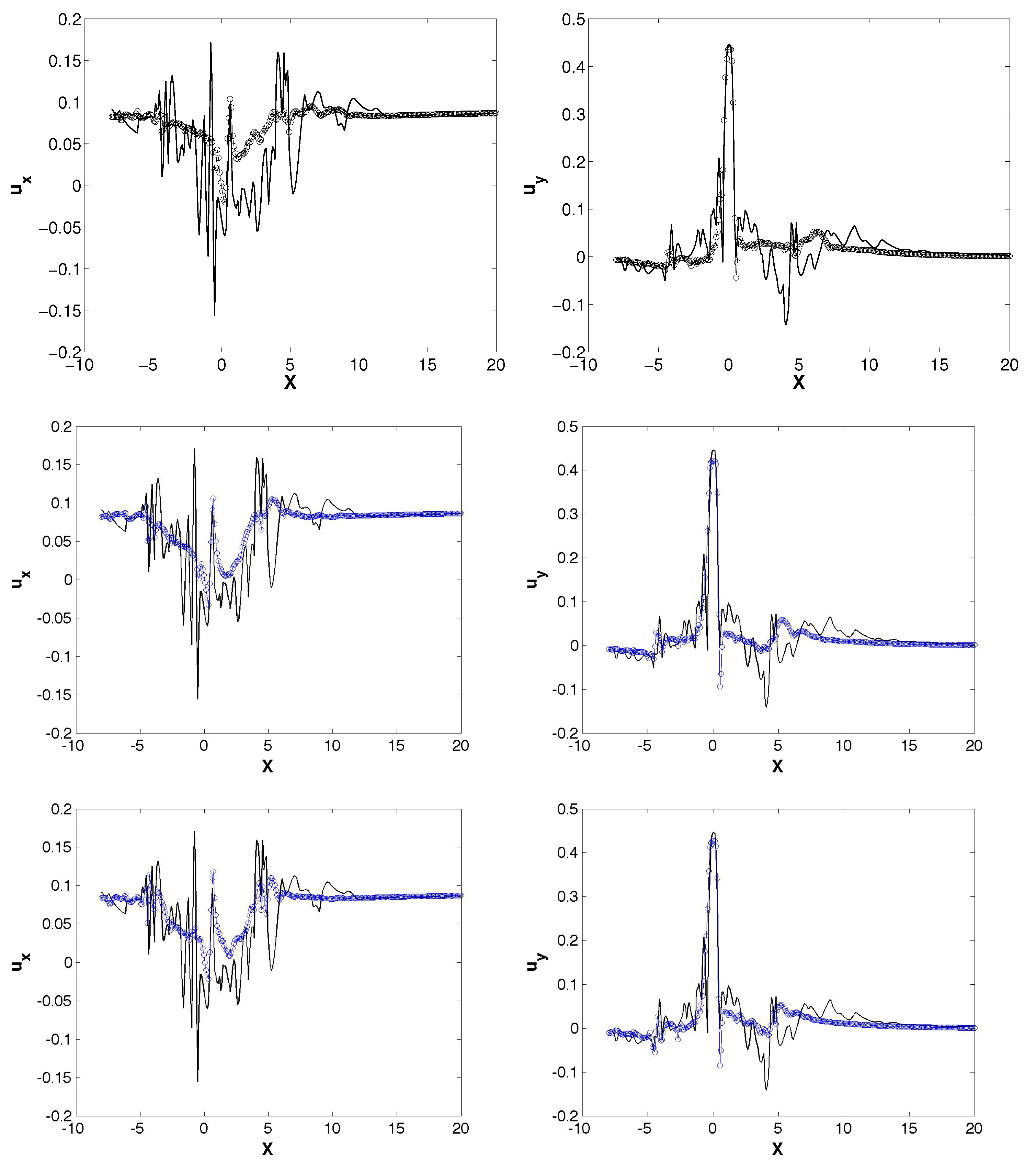
Again, the three HODMD-based ROMs are constructed retaining $M=3$, 5 and 21 DMD modes and the solution is extrapolated in time to $t=202.8$ s. Figure 15 shows the original and the predicted instantaneous flow fields for the three ROMs generated. There is a good agreement between the ROM and the original simulation. The RMS errors for these predictions are ∼40%, ∼41% and ∼44% for $M=3$, 5 and 21, respectively. Figure 16 and Figure 17 show that the model cannot predict the peak values of the velocity fluctuations. When these peaks are removed (i.e., when $x>5$ m), the model predicts the original solution with an RMS error ∼20–25%.

4. Conclusions

We have developed a reduced order model (ROM) to simulate and predict the behaviour of the flow around vertical axis turbines in a turbulent regime. The novel approach requires the simulations of the turbine rotation using a 3D high order solver with a turbulent model of LES type. From this simulation, we extract snapshots to construct the ROM. It has been shown that this method can be computationally efficient and more accurate than low order solvers with simpler turbulent models.

The ROM, which is based on HODMD, requires only a few modes to represent the flow solution in any particular location and time. Even when the sampled snapshots do not cover an entire blade revolution, the resulting ROM is capable of predicting the flow behaviour at any instant in time. The model is validated for a one bladed vertical axis wind turbine in turbulent regime and then extended to the more realistic configuration with three blades at the same turbulent flow conditions.

The developed ROM has been shown to predict accurately the spatial and temporal evolution of flow velocities near the rotating blades but has the potential to replace costly solvers in predicting blade loads or power outputs. This will be explored in further work.

References

1. Ferrer, E.; Willden, R.H.J. Blade-wake interactions in cross-flow turbines. Int. J. Mar. Energy 2015, 11, 71–83. [Google Scholar] [CrossRef]
2. Eriksson, S.; Bernhoff, H.; Leijon, M. Evaluation of different turbine concepts for wind power. Renew. Sustain. Energy Rev. 2008, 12, 1419–1434. [Google Scholar] [CrossRef]
3. Islam, M.; Ting, D.S.K.; Fartaj, A. Aerodynamic models for Darrieus-type straight-bladed vertical axis wind turbines. Renew. Sustain. Energy Rev. 2008, 12, 1087–1109. [Google Scholar] [CrossRef]
4. Tjiu, W.; Marnoto, T.; Mat, S.; Ruslan, M.H.; Sopian, K. Darrieus vertical axis wind turbine for power generation I: Assessment of darrieus VAWT configurations. Renew. Energy 2015, 75, 50–67. [Google Scholar] [CrossRef]
5. Muller, G.; Jentsch, M.F.; Stoddart, E. Vertical axis resistance type wind turbines for use in buildings. Renew. Energy 2009, 34, 1407–1412. [Google Scholar]
6. Newman, B.G. Actuator-disc theory for vertical-axis wind turbines. J. Wind Eng. Ind. Aerodyn. 1983, 15, 347–355. [Google Scholar] [CrossRef]
7. Sagaut, P. Large Eddy Simulation for Incompressible Flows: An Introduction; Scientific Computation; Springer: Berlin, Germany, 2001. [Google Scholar]
8. Rowley, C.W.; Dawson, S.T.M. Model Reduction for Flow Analysis and Control. Annu. Rev. Fluid Mech. 2017, 49, 387–417. [Google Scholar] [CrossRef]
9. Debnath, M.; Santoni, C.; Leonardi, S.; Iungo, G.V. Towards reduced order modelling for predicting the dynamics of coherent vorticity structures within wind turbine wakes. Philos. Trans. R. Soc. A Math. Phys. Eng. Sci. 2017, 375, 20160108. [Google Scholar] [CrossRef] [PubMed]
10. Iungo, G.V.; Santoni-Ortiz, C.; Abkar, M.; Porte-Agel, F.; Rotea, M.A.; Leonardi, S. Data-driven Reduced Order Model for prediction of wind turbine wakes. J. Phys. Conf. Ser. 2015, 625, 012009. [Google Scholar] [CrossRef]
11. Le Clainche, S.; Vega, J.M. Higher Order Dynamic Mode Decomposition. SIAM J. Appl. Dyn. Syst. 2017, 16, 882–925. [Google Scholar] [CrossRef]
12. Kou, J.; Le Clainche, S.; Zhang, W. A reduced-order model for compressible flows with buffeting condition using higher order dynamic mode decomposition with a mode selection criterion. Phys. Fluids 2018, 30, 016103. [Google Scholar]
13. Le Clainche, S.; Vega, J.M. Higher order dynamic mode decomposition to identify and extrapolate flow patterns. Phys. Fluids 2017, 29, 084102. [Google Scholar] [CrossRef]
14. Wang, Z.J.; Fidkowski, R.; Abgrall, K.; Bassi, F.; Caraeni, D.; Cary, A.; Deconinck, H.; Hartmann, R.; Hillewaert, K.; Huynh, H.T.; et al. High-order CFD methods: Current status and perspective. Int. J. Numer. Methods Fluids 2013, 72, 811–845. [Google Scholar] [CrossRef]
15. Ferrer, E.; Willden, R.H.J. A high order Discontinuous Galerkin Finite Element solver for the incompressible Navier-Stokes equations. Comput. Fluids 2011, 46, 224–230. [Google Scholar] [CrossRef]
16. Ferrer, E.; Willden, R.H.J. A high order discontinuous Galerkin—Fourier incompressible 3D Navier-Stokes solver with rotating sliding meshes. J. Comput. Phys. 2012, 231, 7037–7056. [Google Scholar] [CrossRef]
17. Ferrer, E. A high Order Discontinuous Galerkin—Fourier Incompressible 3D Navier-Stokes Solver with Rotating Sliding Meshes for Simulating Cross-Flow Turbines. Ph.D. Thesis, University of Oxford, Oxford, UK, 2012. [Google Scholar]
18. Ferrer, E.; Moxey, D.; Willden, R.H.J.; Sherwin, S. Stability of projection methods for incompressible flows using high order pressure-velocity pairs of same degree: Continuous and discontinuous Galerkin formulations. Commun. Comput. Phys. 2014, 16, 817–840. [Google Scholar] [CrossRef]
19. Ferrer, E. An interior penalty stabilised incompressible discontinuous Galerkin-Fourier solver for implicit Large Eddy Simulations. J. Comput. Phys. 2017, 348, 754–775. [Google Scholar] [CrossRef]
20. Ferrer, E.; de Vicente, J.; Valero, E. Low cost 3d global instability analysis and flow sensitivity based on dynamic mode decomposition and high-order numerical tools. Int. J. Numer. Methods Fluids 2014, 76, 169–184. [Google Scholar] [CrossRef]
21. González, L.; Ferrer, E.; Diaz-Ojeda, H.R. Onset of three dimensional flow instabilities in lid-driven circular cavities. Wind Eng. 2017, 29, 0641022. [Google Scholar] [CrossRef]
22. Ferrer, E.; Le Clainche, S. Flow scales in cross-flow turbines. In CFD for Wind and Tidal Offshore Turbines; Springer International Publishing: Basel, Switzerland, 2015; pp. 1–11. [Google Scholar]
23. Schmid, P.J. Dynamic mode decomposition of numerical and experimental data. J. Fluid Mech. 2010, 656, 5–28. [Google Scholar] [CrossRef] [Green Version]
24. Le Clainche, S.; Vega, J.M.; Soria, J. Higher Order Dynamic Mode Decomposition for noisy experimental data: Flow structures on a Zero-Net-Mass-Flux jet. Exp. Therm. Fluid Sci. 2017, 88, 336–353. [Google Scholar] [CrossRef]
25. Le Clainche, S.; Moreno-Ramos, R.; Taylor, P.; Vega, J.M. A new robust method to study flight flutter testing. J. Aircr. Submitted.
26. Berkooz, G.; Holmes, P.; Lumley, J. The proper orthogonal decomposition in the analysis of turbulent flows. Annu. Rev. Fluid Mech. 1993, 25, 539–575. [Google Scholar] [CrossRef]
27. Kou, J.; Zhang, W. An improved criterion to select dominant modes of dynamic mode decomposition. Eur. J. Mech. B Fluids 2017, 62, 109–129. [Google Scholar] [CrossRef]
28. Sirovich, L. Turbulence and the dynamic of coherent structures, parts I–III. Q. Appl. Math. 1987, 45, 561–571. [Google Scholar] [CrossRef]
29. Le Clainche, S.; Sastre, F.; Vega, J.M.; Velázquez, A. Higher order dynamic mode decomposition applied to postproces a limited amount of PIV data. In Proceedings of the 47th AIAA Fluid Dynamics Conference, AIAA Aviation Forum (AIAA paper 2017-3304), Denver, CO, USA, 5–9 June 2017. [Google Scholar]
30. Le Clainche, S.; Pérez, J.M.; Vega, J.M. Spatio-temporal flow structures in the three-dimensional wake of a circular cylinder. Fluid Dyn. Res. 2018. [Google Scholar] [CrossRef]
31. Sayadi, T.; Schmid, P.J.; Richecoeur, F.; Durox, D. Parametrized datadriven decomposition for bifurcation analysis, with application to thermoacoustically unstable systems. Phys. Fluids 2015, 27, 037102. [Google Scholar] [CrossRef]
32. Bazilevs, Y.; Korobenko, A.; Deng, X.; Yan, J.; Kinzel, M.; Dabiri, J.O. Fluid-structure interaction modeling of vertical-axis wind turbines. J. Appl. Mech. 2014, 81, 081006. [Google Scholar] [CrossRef]
33. Consul, C.A.; Willden, R.H.; McIntosh, S.C. Blockage effects on the hydrodynamic performance of a marine cross-flow turbine. Philos. Trans. R. Soc. A Math. Phys. Eng. Sci. 2013, 371, 20120299. [Google Scholar] [CrossRef] [PubMed]
34. Howell, R.; Qin, N.; Edwards, J.; Durrani, N. Wind tunnel and numerical study of a small vertical axis wind turbine. Wind Eng. 2010, 35, 412–422. [Google Scholar] [CrossRef]
35. Hsu, M.C.; Akkerman, I.; Bazilevs, Y. High-performance computing of wind turbine aerodynamics using isogeometric analysis. Comput. Fluids 2011, 49, 93–100. [Google Scholar] [CrossRef]
36. McLaren, K.; Tullis, S.; Ziada, S. Computational fluid dynamics simulation of the aerodynamics of a high solidity, small-scale vertical axis wind turbine. Wind Energy 2011, 15, 349–361. [Google Scholar] [CrossRef]
37. Qin, N.; Howell, R.; Durrani, N.; Hamada, K.; Smith, T. Unsteady flow simulation and dynamic stall behaviour of vertical axis wind turbine blades. Wind Eng. 2011, 35, 511–527. [Google Scholar] [CrossRef]
38. Fluent Manual—ANSYS Academic Research, Release 16.2; ANSYS, Inc.: Canonsburg, PA, USA, 2015.
39. Oler, J.W.; Strickland, J.H.; Im, B.J.; Graham, G.H. Dynamic Stall Regulation of Thedarrieus Turbine; Technical Report, SANDIA REPORT SAND83-7029 UC-261; Sandia National Laboratories: Albuquerque, NM, USA, 1983. [Google Scholar]
40. Bremseth, J.; Duraisamy, K. Computational analysis of vertical axis wind turbine arrays. Theor. Comput. Fluid Dyn. 2016, 30, 387–401. [Google Scholar] [CrossRef]
41. Chen, Y.; Lian, Y. Numerical investigation of vortex dynamics in an H-rotor vertical axis wind turbine. Eng. Appl. Comput. Fluid Mech. 2015, 1, 21–32. [Google Scholar] [CrossRef]
42. Deglaire, P.; Engblom, S.; Ågren, O.; Bernhoff, H. Analytical solutions for a single blade in vertical axis turbine motion in two-dimensions. Eur. J. Mech. B Fluids 2009, 28, 506–520. [Google Scholar] [CrossRef]
43. Osterberg, D. Multi-Body Unsteady Aerodynamics in 2D Applied to a Vertical-Axis Wind Turbine Using a Vortex Method; Technical Report; Uppsala University: Uppsala, Sweden, 2010. [Google Scholar]
Figure 1. Vertical axis turbine flow fields: (a.1) high order Discontinuous Galerkin mesh with P = 3 (high order polynomial nodes are shown in red); (b.1) low order mesh; (a.2) high order DG numerical solution (LES) and (b.2) low order numerical solution (uRANS). Contours show streamwise velocity ( u x ) with 10 levels from 0 to 0.2.
Energies 11 00566 g001
Figure 2. Normal force coefficient for a vertical axis turbine: (a) 3D high order DG simulation (LES turbulence model); (b) low order fluent simulation (k-omega SST turbulence model. Both compared to experimental data [39] for four turbine revolutions.
Energies 11 00566 g002
Figure 3. Simulations of vertical axis turbine: Flow velocity components at lines: (a.1) streamwise velocity u x at y = 2 m, (a.2) normal velocity u y at y = 2 m; (b.1) streamwise velocity u x at y = 4 m, (b.2) normal velocity u y at y = 4 m. We include results from the 3D high order DG simulation (LES turbulence model) and from the low order fluent simulation k-omega SST turbulence model.
Energies 11 00566 g003
Figure 4. One-blade turbine case: temporal evolution of the streamwise (top) and normal (bottom) velocity fields, u x and u x for points P ( x 1 , y 1 ) = ( 0 , 4 ) (left) and P ( x 1 , y 1 ) = ( 2.8 , 2 ) (right) (see the computational domain in Figure 1).
Energies 11 00566 g004
Figure 5. One-blade turbine case: growth rates (left) and amplitudes (right) vs. frequencies of the DMD modes. Circles represent the modes selected by HODMDc for constructing the HODMD-based Reduced Order Model (ROM) and crosses represent the transient modes, omitted in the DMD expansion (1).
Energies 11 00566 g005
Figure 6. One-blade wind turbine case: streamwise (left) and normal (right) velocities, u x and u y , of the instantaneous flow field at time instant 240 s. Two-dimensional x y cross section at z = 0.9375 m.
Energies 11 00566 g006
Figure 7. One-blade wind turbine case: temporal evolution of streamwise (left) and normal (right) velocities in y = 4 m at time instant 240 s. From top to bottom: HODMD-based ROM constructed using M = 3, 5 and 21 DMD modes. Continuous black line and blue circles represent the original and the predicted solution, respectively.
Energies 11 00566 g007
Figure 8. Counterpart of Figure 7 in y = 2 .
Energies 11 00566 g008
Figure 9. Counterpart of Figure 4 in the three-blades turbine in points P ( x 1 , y 1 ) = ( 0 , 4 ) (left) and P ( x 1 , y 1 ) = ( 2 2 , 2 2 ) (right).
Energies 11 00566 g009
Figure 10. Counterpart of Figure 5 in the three-blades turbine applying HODMD in 196 snapshots starting at time 80.1 s.
Energies 11 00566 g010
Figure 11. Counterpart of Figure 6 in the three-blades turbine applying HODMD in 196 snapshots starting at time 80.1 s.
Energies 11 00566 g011
Figure 12. Counterpart of Figure 7 in the three-blades turbine applying HODMD in 196 snapshots starting at time 80.1 s. Data extracted at y = 2 2 m.
Energies 11 00566 g012
Figure 13. Counterpart of Figure 7 in the three-blades turbine applying HODMD in 196 snapshots starting at time 80.1 s. Data extracted at y = 2 2 m.
Energies 11 00566 g013
Figure 14. Counterpart of Figure 5 the three-blades turbine applying HODMD in 145 snapshots starting at time 25.604 s.
Energies 11 00566 g014
Figure 15. Counterpart of Figure 6 in the three-blades turbine applying HODMD in 145 snapshots starting at time 25.604 s.
Energies 11 00566 g015
Figure 16. Counterpart of Figure 7 in the three-blades turbine applying HODMD in 145 snapshots starting at time 25.604 s. Data extracted at y = 4 m.
Energies 11 00566 g016
Figure 17. Counterpart of Figure 7 in the three-blades turbine applying HODMD in 145 snapshots starting at time 25.604 s. Data extracted at y = 2 2 m.
Energies 11 00566 g017aEnergies 11 00566 g017b