Economic Value Assessment and Optimal Sizing of an Energy Storage System in a Grid-Connected Wind Farm

Abstract

This study identifies the optimal management policy of a given energy storage system (ESS) installed in a grid-connected wind farm in terms of maximizing the monetary benefits and provides guidelines for defining the economic value of the ESS under optimal management policy and selecting the optimal size of the ESS based on economic value. Considering stochastic models for wind power and electricity price, we develop a finite-horizon periodic-review Markov decision process (MDP) model to seek the optimal management policy. We also use a simple optimization model to find the optimal storage capacity and charging/discharging capacity of the ESS. By applying our analytic approach to a real-world grid-connected wind farm located in South Korea, we verify the usefulness of this study. Our numerical study shows that the economic value of the ESS is highly dependent on management policy, wind electricity variability, and electricity price variability. Thus, the optimal size of ESS should be carefully determined based on the locational characteristics and management policy even with limited investments. Furthermore, this study provides a meaningful policy implication regarding how much of a subsidy the government should provide for installing ESS in a wind farm.

1. Introduction

As greenhouse gas emission reduction has recently received extensive attention, renewable energy resources have been rapidly integrated into the electricity sector around the world. Several countries, including South Korea, Britain, Italy, Poland, Belgium, and Chile, as well as most states of the U.S., have aggressively adopted renewable policies such as renewable portfolio standard (RPS). According to a recent report published by the International Energy Agency (IEA), renewable energy resources will account for the largest portion of total primary energy consumption in the global electricity sector in 2030 [1]. The report projects that wind energy will make the largest contribution to the penetration.

As the penetration level of the wind energy in an electric power system increases, the critical weak points of the wind energy—intermittency and non-dispatchability—have posed more challenges in the operation of the electric power system in terms of the quality of power, liability, and so on. As attempts to overcome these challenges, new technologies have been developed, such as a smart grid and/or an energy storage system (ESS). In particular, with recent technological advancement and reduced costs, integration of the battery-based energy storage system (BESS) into the electric power system has begun in many regions. According to a database from the U.S. Department of Energy [2], many wind farms adopted ESS in the U.S., Europe, and China. In western Texas (U.S.), 36 MW and 0.67 h duration ESS was installed at the 153 MW Notrees wind power project, 2 MW and 1 h duration ESS was installed at the 18 MW Bosch wind power project in the northern Germany, and five serial ESS projects, in total 16 MW/71 MWh, were invested for a hybrid system with 500 MW wind and 100 solar PV capacities in Zhangbei, China.

In South Korea, the government has developed a plan to actively expand the use of renewable energy in the electricity sector. One goal of the plan announced in 2014 is to increase the portion of renewable energy resources in the electricity sector from 3.66% in 2012 to 13.4% in 2035. Among renewable energy resources, wind energy is expected to account for the largest portion (more than 30%) in 2030 [3]. Accordingly, a national renewable energy policy mandates the RPS for power producers whose installed capacity is over 500 MW. In particular, Jeju Island, home to more than 650,000 people, has a plan to generate electricity from only renewable energy sources and considers wind turbines as the primary renewable sources.

As a way to resolve the weak points of the wind energy, the Korean government has encouraged the adoption of ESS by giving a high subsidy to a wind farm that has its own ESS. In 2016, a power supplier with ESS connected to a wind farm can receive five renewable energy certificates (RECs) for a unit of electricity generated during the peak period under the Korean RPS policy. On the other hand, a wind farm without ESS receives only one REC for a unit of electricity generated. In 2015, Jeju Island legislated that a new wind farm must have its own ESS, and its charging/discharging capacity should be larger than 10% of the nameplate capacity of the wind farm.

The literature on ESS reveals that the lack of adequate information on ESS economy is a major obstacle in building feasible business models and regulation strategies such as government subsidies [4,5,6]. Despite a considerable policy support for promoting ESS, its sizable adoption has not been achieved because its economic feasibility is questionable in practice. This low economic feasibility is mainly due to the high upfront cost of installing ESS. Moreover, arbitrary decisions made about operations and size of ESS worsen the economic viability. For example, Walawalkar and Apt [7] reported that only 2.5% of the total power delivered in the U.S. passed through an ESS while there were over 200 GW of installed ESS capacity. This non-optimal size adding to the high upfront cost may prevent acceptable economic feasibility of each ESS. Thus, a valid economic evaluation of ESS should be made on the basis of how to adequately size and operate it.

While the ESS size and operations have significant effects on its economic value, to the best of our knowledge, no research has considered how to determine ESS size together with its optimal management policy in the context of assessing economic benefits in a grid-connected wind farm. This study attempts to make a contribution to the literature by addressing this problem. We first identify a management policy for optimally operating the ESS. Considering the inter-temporal nature of ESS operations (i.e., the operation in one time step will affect its operation in the others), we employ a dynamic programming approach for the problem. In particular, to accommodate the uncertainty associated with electricity price and wind energy, we formulate the problem as a Markov Decision Process (MDP) model and find the optimal management policy. The problem has, fortunately, similar structural properties with traditional inventory control problems [8], which are typically formulated as MDP models [9,10,11]. Within the MDP model, we define how to assess the economic value of the ESS and find an optimal ESS size that maximizes its economic value. This work finally simulates the effects of several factors such as electricity price and demand on the economic value in a grid-connected wind farm.

The rest of this paper is organized as follows. We first review the relevant literature on wind-ESS hybrid systems and the related optimization models and emphasize our new contributions in Section 2. We introduce a finite-horizon MDP model to identify an optimal management policy for operating the ESS in Section 3, followed by the structural analysis of the optimal management policy in Section 4. Section 5 describes the economic value of the ESS under the optimal management policy and how to decide the optimal size of the ESS based on the economic value. In Section 6, for a verification purpose of our analytical results, we conduct an extensive numerical study with real data compiled from a wind farm located in South Korea and the Korean electricity market. Lastly, conclusions and discussions are presented in Section 7.

2. Literature Review

This section summarizes the recent research progress in assessing the economic value of ESS and the related decision-making problems. Even though a very large number of previous studies exist, we only focus on studies dealing with the economic aspect of the ESS in a grid-connected wind-ESS hybrid system, particularly. Two previous studies can provide more general reviews covering several aspects, including power fluctuation mitigation, frequency regulation, and so on [12,13]. In comparison with previous literature, we clarify the contributions of this research and briefly describe the regulatory framework on the ESS operation and relevant studies in Korea.

2.1. Summary of Methodological Advance

Since the mid-2000s, several studies have considered the effective use of ESS regarding the interplay of wind turbines, energy storage, and transmission capacity and the evaluation of its economic value [13,14,15,16]. These studies were based on deterministic sample paths of electricity price and wind energy dynamics by analyzing historical data. By conducting extensive sensitivity analysis for various sizes of the ESS in the hybrid system, they evaluated the economic value for a specific ESS size and found the optimal size of the ESS through the simple cost-benefit analysis. The types of ESS considered in the papers are the compressed air energy storage (CAES) [13,14,15] and the battery energy storage [13,16]. However, they have not considered the effect of the management policy of the ESS, which can vary its economic value.

To find the optimal management policy of the ESS in the hybrid system, several studies have employed deterministic optimization models. The deterministic models assume that the future values of electricity spot price, demand load and wind energy generations are known. Korpaas et al. [17] characterized an optimal strategy for ESS operation and sizing an on-site ESS with given capacities of a wind farm and transmission to the external grid, and a known demand distribution. They used a dynamic programming approach to analyze the strategy. Brekken et al. [18] considered a large wind farm integrated with an on-site zinc-bromine flow battery, with the objective of meeting an hour-ahead predicted power output to a large grid. They focused on the total costs of the entire grid rather than the hybrid system and ignored the transmission capacity between the hybrid system and the grid. It was shown that an optimal operation strategy could result in significantly lower costs than a simple strategy. Zhang and Li [19] used a two-scale dynamic programming scheme and considered the least-cost management policy of a wind-ESS hybrid system, assuming that local demand was known and the ESS was allowed to charge the electricity from the utility grid. Luo et al. [20] and Bridier et al. [21] also optimally determined the ESS size and its management policy for a system similar to the system considered in this study (see Section 3). Both studies applied heuristic approaches to solve their deterministic models.

However, some researchers and practitioners have criticized the critical limitation of previous studies because they ignored the uncertainty associated with electricity spot price and wind energy. This uncertainty can significantly affect the assessment of the economic value and the decision-making problems. Taking into account the uncertainty, several papers have suggested methodologies for the optimal sizing and/or management of the ESS. Some studies used MDP models and stochastic dynamic programming approaches to find an optimal ESS management policy and evaluate its economic value based on the policy. Shu and Jirutitijaroen [22] found the optimal policy from their stochastic MDP model. They showed that the policy could lead to considerably higher profits than an optimal policy derived from a deterministic model because the deterministic model underestimated the economic value of the ESS. Kim and Powell [23] derived a mathematical form for an optimal management policy of an ESS in a wind farm assuming simple probability distributions for uncertain factors. They used the policy to study the economics of the storage capacity. Similarly, Zhou et al. [24] suggested an optimal policy for operating a wind-ESS hybrid system with limited transmission capacity and quantified the economic value of the ESS under the policy. However, the optimal ESS size under uncertainty was not the main consideration in those studies, and this could be critical for installing a new ESS. Harsha and Dahleh [25] defined the economic value of the ESS as reductions in the long-run average cost by using the ESS based on an infinite-horizon MDP model and examined the trade-off between the value and capital costs of the storage in a simple convex optimization problem to find the optimal ESS size.

Contrary to previous studies, we introduce a way to determine the optimal ESS size that maximizes the economic value of ESS.

Table 1. The literature on optimizing an energy storage system (ESS) in a wind farm.

	Electricity Price & Wind Energy Dynamics	Optimal Management Policy	Optimal Sizing	ESS Technology
Denholm and Sioshansi [14]	deterministic profiles	not considered	considered	Compressed air energy storage
Fertig [15]	deterministic profiles	not considered	considered	Compressed air energy storage
Johnson et al. [16]	deterministic profiles	not considered	considered	Radox and sodium sulfur battery
Berrada and Loudiyi [13]	deterministic profiles	not considered	considered	multiple technologies
Korpaas et al. [17]	deterministic profiles	deterministic optimization	considered	not specified
Brekken et al. [18]	deterministic profiles	deterministic optimization	not considered	Zinc-bromine flow battery
Zhang and Li [19]	deterministic profiles	deterministic optimization	not considered	Li-ion battery
Luo et al. [20]	deterministic profiles	deterministic optimization	considered	Li-ion battery
Bridier et al. [21]	deterministic profiles	deterministic optimization	considered	not specified
Shu and Jirutitijaroen [22]	stochastic models	finite-horizon MDP	not considered	Compressed air energy storage
Kim and Powell [23]	Stochastic models	infinite-horizon MDP	not considered	general battery
Zhou et al. [24]	Stochastic models	finite-horizon MDP	not considered	general battery
Harsha and Dahleh [25]	Stochastic models	infinite-horizon MDP	considered	not specified
Our study	Stochastic models	finite-horizon MDP	considered	Li-ion battery

summarizes the literature review and emphasizes how our study is different with previous studies. We mainly refer to the work in [24,25] when formulating an MDP model in Section 3. However, we consider that the ESS cannot charge the electricity transmitted from the utility grid because it is more suitable for the Korean regulatory framework (see Section 2.2).

2.2. Studies in Korea

Under the Korean regulatory framework, a grid-connected wind farm is allowed to sell its generated electricity through a wholesale electricity market, operated by Korea Power Exchange (KPX), if it has more than 1000 kW nameplate capacity. The electricity generated by a wind-ESS hybrid system is sold at the system marginal price (SMP), along with additional benefits such as high tradeable RECs and investment and production tax credits [26,27]. Thus, wind-ESS hybrid systems are not allowed to purchase electricity from the grid to receive the benefits. If the ESS is able to charge electricity from the grid to provide an arbitrage opportunity, the ESS becomes an individual power provider who is likely to increase its profit only by trading electricity with the grid instead of being a tool to promote wind energy. Several previous studies in Korea considered a situation where the electricity transmission from a wind-ESS hybrid system to grid is allowed, but the reverse is not [28,29,30].

To the best of our knowledge, little research has simultaneously considered the economic value assessment and optimal sizing of the ESS in Korea. Only a few studies have suggested a simple method for determining the ESS size. Lim [31] presented a simple linear programming model to design the optimal ESS size in a hybrid system consisting of solar PV, wind and tidal. Cho et al. [32] proposed a heuristic method for the optimal sizing of a demand side customer’s battery storage system. Therefore, this study contributes to the limited literature and supports decision-makers by providing tangible research outcomes based on real data from a wind farm in Korea.

3. Optimal ESS Management Policy Model

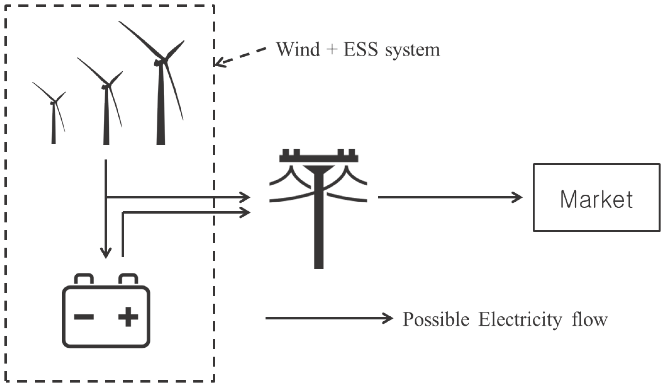
In this study, we consider a grid-connected hybrid system as shown in Figure 1. The hybrid system has several wind turbines (a wind farm) and an ESS, and the system is connected to a large utility grid via a transmission line. The system can sell all the generated electricity to a wholesale market on the grid assuming that the amount of generated electricity is negligible compared to the total amount of electricity on the grid. The generated electricity is sold at SMP on the wholesale electricity market and the amount does not affect the SMP values. It is also assumed that the electricity from the grid cannot be transmitted to the hybrid system through the transmission line as in the Korean regulatory framework described in Section 2. Here, the electricity generated from the turbines cannot be accurately anticipated due to uncertain wind speed, but the ESS will save some electricity from the farm to provide the electricity to the grid when the wind turbines cannot generate enough electricity. Thus, the stored electricity can be sold to increase the profit of the wind farm when the SMP is relatively high.

For this situation, we first identify the optimal operating policy of the ESS in the hybrid system. The operator of the system needs to periodically make decisions on the optimal level of stored electricity subject to the wind power availability, ESS capacity, SMP price, and transmission capacity. That is, under uncertainty of wind power generation and SMP price, the system makes decisions periodically over a finite horizon, at each time t in the finite set $T:=0,\tau ,\dots ,T-\tau$ (that is, the length of time interval is $\tau$). Assuming that the wind power is a Markov process and the SMP value at a specific time period follows a probabilistic distribution, an MDP model is used to sequentially make the decisions in this paper. Therefore, we consider this problem as a period-review inventory management problem where decisions are made at equally spaced points in time, and we develop a finite-horizon periodic-review MDP model as follows:

Parameters:

• S: storage capacity of the ESS (in energy units, e.g., MWh).
• W: nameplate capacity of the wind farm (in energy unit/period, e.g., MW).
• $R_i$, $R_o$: charging and discharging capacity of the ESS in a specified period, respectively (in energy units/period, e.g., MW).
• ${\rho }_i$, ${\rho }_o$: charging and discharging efficiency of the ESS, respectively (${\rho }_i$, ${\rho }_o$ $\in (0,1]$). Each accounts for the storage conversion losses, and the round-trip efficiency is then $\rho ={\rho }_i{\rho }_o$ ($\rho \in (0,1]$).
• $C^T$: transmission capacity (in energy unit/period, e.g., MW).
• $\eta$: transmission efficiency, the ratio of energy dissipated by the load to the transmission line.
• $\delta$: one-period risk-free discount rate ($0<\delta \le 1$)

Generally, the charging and discharging capacities are the same, $R_i=R_o$, so we assume that $R=R_i=R_o$ in this study.

State Variables:

The period t is defined as the time interval $[t,t+\tau )$. We assume that the state variables with subscript t are realized at the beginning of period t. For example, the amount of wind electricity generated in the time interval $[t,t+\tau )$ is known at time t, denoted by $w_t$. It is assumed that the $w_t$ is followed by a well-known stochastic process after t. In this work, we use an exogenously defined Markovian process to model $w_t$. In addition, the electricity price at time period t, denoted by $p_t$, is assumed to follow a pre-defined electricity SMP pattern. Thus, the state at time t is defined by the following variables:

• $x_t$: the level of available electricity in the ESS at the beginning of period t (in energy units, e.g., MWh) ($x_t\in [0,S]$).
• $w_t$: the wind electricity generated in time period t (in energy units, e.g., MWh) ($w_t\in [0,\tau W]$).
• $p_t$: the electricity price at time t, which will not be changed during the time period $[t,t+\tau )$ (in currency unit/energy units, e.g., $/MWh)

The tuple $E_t=\{x_t,w_t,p_t\}$ forms the state of our problem.

Decision Variable:

• $a_t$: the amount of electricity to charge/discharge at time period t (in energy units, e.g., MWh).

It is positive when the electricity is stored (if $a_t>0$, charging) and negative when a part of stored electricity is withdrawn to be sold (if $a_t<0$, discharging). Assume that there is no way to buy and store electricity from the grid, that is, electricity generated only by wind turbines can be stored:

State Transition:

• $x_{t+1}=x_t+a_t,$
• $w_{t+1}=g_1(w_t)$ and $p_{t+1}=g_2(p_t).$

The level of available electricity in the ESS at time period $t+1$ changes depending on the amount of electricity to charge/discharge at time period t. The state variables $w_t$ and $p_t$ evolve to $w_{t+1}$ and $p_{t+1}$ according to their respective exogenous stochastic process, expressed as known functions $g_1(·)$ and $g_2(·)$, and we assume that they are mutually independent.

Immediate Payoff Function and Constraints:

Let $f(a_t,x_t,p_t,w_t)$ be the immediate payoff function at time t, defined as

$$\begin{array}{c}\hfill f(a_t,x_t,p_t,w_t)=\left\{\begin{array}{cc}{p}_t·min\left[{(w_t-a_t/{\rho }_i)}^{+},\tau C^T\right]·\eta ,\hfill & \mathrm{if}{a}_t\ge 0,\hfill \\ p_t·min\left[{(w_t-{\rho }_o{a}_t)}^{+},\tau C^T\right]·\eta ,\hfill & \mathrm{if}{a}_t<0.\hfill \end{array}\right.\end{array}$$

When a part of wind electricity generated at time t is stored ($a_t\ge 0$), the selling amount can be smaller than the generated electricity at time t. If a part of the stored electricity is extracted and delivered ($a_t<0$), the total amount of electricity sold at time t becomes the generated wind electricity plus the electricity extracted from the storage at time t. In both cases, the amount of electricity to sell cannot be greater than the given transmission capacity. To specify feasible values of $a_t$, we consider several constraints as follows:

• When $a_t\ge 0$,

  $$\begin{array}{c}\hfill \left\{\begin{array}{cc}{x}_t+a_t\le S\hfill & :\mathrm{storage}\mathrm{capacity},\hfill \\ a_t\le {\rho }_i·w_t\hfill & :\mathrm{wind}\mathrm{electricity}\mathrm{generation},\hfill \\ a_t\le \tau R\hfill & :\mathrm{ramping}\mathrm{constraint}-\mathrm{charging}\mathrm{rate},\hfill \end{array}\right.\end{array}$$
• When $a_t<0$,

  $$\begin{array}{c}\hfill \left\{\begin{array}{cc}-a_t\le x_t\hfill & :\mathrm{ESS}\mathrm{stored}\mathrm{electricity}\mathrm{availability},\hfill \\ -a_t\le \tau R\hfill & :\mathrm{ramping}\mathrm{constraint}-\mathrm{discharging}\mathrm{rate}.\hfill \end{array}\right.\end{array}$$

These constraints can be combined by

$$\begin{array}{c}\hfill \mathrm{s}.\mathrm{t}.max(-x_t,-\tau R)\le a_t\le min\left(S-x_t,{\rho }_i{w}_t,\tau R\right).\end{array}$$

Objective Function:

Our objective is to maximize the total discounted expected cash flows, monetary benefits that the grid operator can make by selling the electricity into the grid, over all feasible decisions:

$$\underset{\pi \in \mathsf{\Pi }}{max}\sum _{t=0}^{T-1}{\delta }^t\mathbb{E}[f(a_t^{\pi },x_t,p_t,w_t)|E_o],$$

(1)

where $\pi$ is a feasible policy that is a sequence of decisions, and $\mathsf{\Pi }$ is the set of all feasible policies. The expectation is taken with respect to the distribution of the random state $E_t$ in time period t. The exogenously determined stochastic models for wind electricity and electricity price induce the distribution, and the value function of the optimal management policy for state $E_t$ in each time period t is defined as

$$V_t^{\ast }(E_t)=\underset{a_t}{max}f(a_t,x_t,p_t,w_t)+\delta \mathbb{E}[V_{t+1}(x_t+a_t,w_{t+1},p_{t+1})|E_t].$$

(2)

In addition, we assume that the remaining electricity in the ESS at the end of time period T is worthless, that is, $V_T^{\ast }(E_T)=0,\forall E_T$.

4. Analysis of Optimal ESS Management

We now proceed to investigate structural properties of the optimal management policy of the ESS. In particular, we analyze charging/discharging action, $a_t^{\ast }(E_t)$, of the MDP model defined in Section 3, with a given storage and charging/discharging capacities, denoted by S and R, respectively. If the electricity prices and the amount of wind electricity generated are known in advance, the optimal management policy can be easily determined by using the deterministic dynamic programming. However, since we assume that both the electricity price and the wind electricity generated follow the exogenous stochastic processes, the ESS management policy should consider their variabilities. In addition, the ramp constraints from the charging/discharging capacities of the ESS and the maximum electricity sale constraint from the transmission capacity raise other concerns about the optimal management policy.

The structure of the optimal management policy can be established in a way that is similar to previous studies [24,25]. To derive the optimal management policy, $a_t^{\ast }(E_t)$, the well-defined stochastic models for wind electricity generation and electricity price are incorporated into the MDP model, so the optimal ESS management decision at each time period can be found using standard backward recursion. Before we analyze the optimal management policy, in a way that is similar to the proofs of Lemma 1 and Proposition 2 in the study of Zhou et al. [24], we could see a property that the value function $V_t^{\ast }(E_t)$ is a non-decreasing and concave function in the level of available electricity in the ESS, $x_t$, given any wind electricity generated $w_t$ and the electricity price $p_t$. This property implies that, without the holding cost for the electricity stored in the ESS, the more electricity the ESS has, the greater the monetary benefit. Moreover, the marginal benefit decreases with a higher level of electricity. With this property, we show that the optimal management policy has different dual-threshold structures depending on the two state variables $x_t$ and $w_t$. We also show that these dual-threshold levels are functions of two state variables $w_t$ and $p_t$. Three cases are possible for which the two state variables $x_t$ and $w_t$ represent different situations, and the optimal management policy has different dual threshold structures. Figure 2 illustrates these cases.

Case 1, $(x_t,w_t)\in (A1)$, represents a situation where the amount of the wind electricity generated in time period t is very large; thus, even though the ESS is charged as much as possible, the remaining electricity is still larger than the maximum transmittable amount of electricity through the transmission line to the grid. Secondly, case 2, $(x_t,w_t)\in (A2)$, represents a situation where the amount of the wind electricity generated in time period t is large, but, if the ESS is charged as much as possible, all of the remaining electricity can be transmitted to the grid. Lastly, case 3, $(x_t,w_t)\in (A3)$, represents a situation, where the wind electricity generated in time period t is less than the maximum transmittable amount of electricity through the transmission line to the grid. Proposition 1 establishes the structure of the optimal management policy, and its proof is provided in Appendix A.

Table 2. Situations and corresponding optimal ESS management policies in three cases.

Case	Situation and Optimal Action (Proposition 1)
Case 1	Situation : wind electricity ≥ transmittable and storable electricity
	($w_t\ge \tau C^T+min\{\tau R,S-x_t\}/{\rho }_i$)
(A1)	Optimal Action : store as much as possible
Case 2	Situation : transmittable electricity ≤ wind electricity < transmittable and storable electricity
	($\tau C^T\le w_t<\tau C^T+min\{\tau R,S-x_t\}/{\rho }_i$)
(A2)	Optimal Action : store up to $\underline{x_t}$ and sell remains, or sell as much as possible and store remains
Case 3	Situation : wind electricity < transmittable electricity
	$(w_t<\tau C^T)$
(A3)	Optimal Action : store up to $\underline{x_t}$, do nothing, or sell down to $\overline{x_t}$

summarized the situations and corresponding optimal ESS management policies in three cases.

Proposition 1.

The optimal charging/discharging action at time period t, $a_t^{\ast }(E_t)$, is determined by two threshold functions, $\overline{x_t}(w_t,p_t)$ and $\underline{x_t}(w_t,p_t)$, as follows:

$$\begin{array}{cc}\hfill \mathrm{case}1:if(x_t,w_t)\in (A1),a_t^{\ast }(E_t)& =min\{\tau R,S-x_t\},\hfill \end{array}$$

(3)

$$\begin{array}{cc}\hfill \mathrm{case}2:if(x_t,w_t)\in (A2),a_t^{\ast }(E_t)& =\left\{\begin{array}{cc}min\{\underline{x_t}-x_t,\tau R\},\hfill & if{x}_t\in [0,{(\underline{x_t}-(w_t-\tau C^T){\rho }_i)}^{+}],\hfill \\ (w_t-\tau C^T){\rho }_i,\hfill & if{x}_t\in [{(\underline{x_t}-(w_t-\tau C^T){\rho }_i)}^{+},S],\hfill \end{array}\right.\hfill \end{array}$$

(4)

$$\begin{array}{cc}\hfill \mathrm{case}3:if(x_t,w_t)\in (A3),a_t^{\ast }(E_t),& =\left\{\begin{array}{cc}min\{\underline{x_t}-x_t,w_t{\rho }_i,\tau R\}\hfill & if{x}_t\in [0,\underline{x_t}],\hfill \\ 0\hfill & if{x}_t\in [\underline{x_t},\overline{x_t}]\hfill \\ max\{\overline{x_t}-x_t,(w_t-\tau C^T)/{\rho }_o,-\tau R\}\hfill & if{x}_t\in [\overline{x_t},S],\hfill \end{array}\right.\hfill \end{array}$$

(5)

where, when $y_t=x_t+a_t$ (the ending level of available electricity in the ESS), the two thresholds can be defined as follows:

$$\begin{array}{cc}\hfill \mathit{store}-\mathit{up}-\mathit{to}\mathit{level}:\underline{x_t}& ={argmax}_{y_t\in [0,S]}-p_t{y}_t/{\rho }_i+\delta \mathbb{E}[V_{t+1}(y_t,w_{t+1},p_{t+1})],\hfill \end{array}$$

(6)

$$\begin{array}{cc}\hfill \mathit{sell}-\mathit{down}-\mathit{to}\mathit{level}:\overline{x_t}& ={argmax}_{y_t\in [0,S]}-p_t{y}_t{\rho }_o+\delta \mathbb{E}[V_{t+1}(y_t,w_{t+1},p_{t+1})].\hfill \end{array}$$

(7)

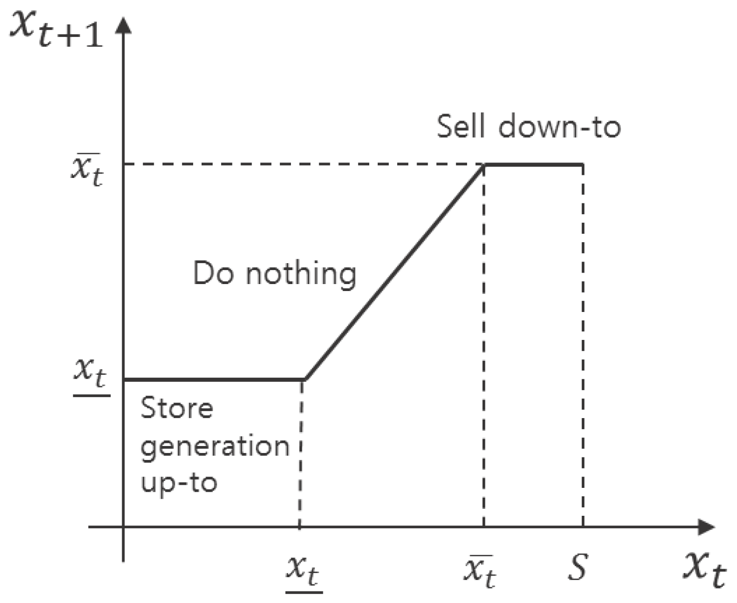
Note that, when we have the charging/discharging efficiencies, ${\rho }_i,{\rho }_o$, the optimal management policy has a two-threshold structure. If ${\rho }_i={\rho }_o=1$, then the two thresholds are the same, $\underline{x_t}=\overline{x_t}$. Under the two-threshold structure, the optimal charging/discharging action in Proposition 1 implies the following situations. In case 1, $(x_t,w_t)\in (A1)$, a part of the large amount of the wind electricity generated at the time period t will be transmitted to the grid as the maximum transmission capacity, $\tau C^T$, another part of the wind electricity will be charged into the ESS as much as possible, and the remaining part of the wind electricity will be curtailed. In case 2, $(x_t,w_t)\in (A2)$, the amount of the wind electricity generated at the time period t, at most $\tau C^T$ amounts will be transmitted into the grid and at least $(w_t-\tau C^T)$ amounts will be charged into the ESS. If the level of available electricity in the ESS at the beginning of the time period is low enough, then the ESS will be charged up to the store-up-to level. In case 3, three possibilities exist. First, some parts of the wind electricity generated at the time period t will be charged and the other parts of the wind electricity will be transmitted into the grid when the level of available electricity in the ESS at the beginning of the time period is low enough. Second, all wind electricity generated at the time period t will be transmitted into the grid when the level of available electricity in the ESS at the beginning of the time period is between the store-up-to level and the sell-down-to level. Finally, not only will all wind electricity generated at the time period t be transmitted into the grid, but also some parts of the electricity stored in the ESS will be discharged and transmitted into the grid when the level of available electricity in the ESS at the beginning of the time period is high enough. Figure 3 shows the structure of optimal charging/discharging action of the ESS in case 3.

5. Economic Value and Optimal Sizing of ESS

This section presents the way to assess the economic value of ESS under the optimal storage management policy established in the previous section and to find its optimal size based on the economic value. The profit at a wind farm is made by selling electricity generated by wind turbines or stored in storage facilities. For a given size of ESS, the amount of electricity sold at time period t can be optimally determined taking into account the variabilities of wind electricity and electricity price as described in the previous Section 4. It is obvious that the value function without ESS ($S=0$) is less than that with ESS ($S>0$). We estimate the economic value of ESS by computing the difference between the value functions with ESS and without ESS. Assuming that the investment cost for ESS depends not only on storage capacity S but also charging/discharging capacity R, we define the cost function in a simple way, as in previous studies [18,33]. As the storage capacity, S, and the charging/discharging capacity, R, of the ESS are considered as the decision variables, the optimization problem to maximize the net profit can be formulated as follows:

$$\underset{S,R}{max}\left({\mathbb{E}}_{p_t,w_t}\left[{{\displaystyle \sum }}_{t=0}^{T-1}{\delta }^t{p}_{t}min[{(w_t+a_t{\beta }_t)}^{+},\tau C^T]·\eta \right]-{\mathbb{E}}_{p_t,w_t}\left[{{\displaystyle \sum }}_{t=0}^{T-1}{\delta }^t{p}_{t}min(w_t,\tau C^T)\right]-(c_{s}S+c_{r}R)\right),$$

(8)

where $c_s$ and $c_r$ are the unit capital costs for the storage capacity and the charging/discharging capacity of ESS, respectively. Here, ${\beta }_t$ represents the charging/discharging efficiencies, i.e., $-1/{\rho }_i$ if $a_t\ge 0$ and $-{\rho }_o$ if $a_t<0$. Since the wind electricity and electricity price are not deterministic, we take the average profit under the optimal management policy of ESS. The first term of the function above is the average profit made by selling electricity with ESS. On the other hand, the second term is the average profit without ESS when all amounts of electricity generated at time period t are sold at the current price $p_t$. As a result, the difference between the first term and second term is defined as the economic value of ESS. The third term is the investment cost for storage over the time horizon, T.

In general, the value of the first term cannot be simply estimated because the optimal value of $a_t$ with a specified size of ESS must be first obtained, as we described in Section 4. Thus, we consider the two-stage optimization approach. At the first stage, a specified size of ESS, (S, R) is fixed, and then the optimal management policy of the ESS is determined at the second stage to compute the average values in Equation (8). By testing various ESS sizes, the optimal ESS size will be searched. For our analysis, it is useful to define the following function with $a_t^{\ast }(S,R)$, which is the optimal $a_t$ with a given size (S, R):

$$\begin{array}{c}\hfill f(S,R)={\mathbb{E}}_{p_t,w_t}\left[\sum _{t=0}^{T-1}{\delta }^t{p}_{t}min[{(w_t+a_t^{\ast }(S,R){\beta }_t)}^{+},\tau C^T]·\eta \right].\end{array}$$

(9)

In fact, this function is equivalent to the optimal value of the first term of Equation (8) and indicates the average profit with the optimal ESS management policy under a given size (S, R). According to Theorems 11 and 12 of Harsha and Dahleh [25] and our numerical results in Section 6, we could see a property where $f(S,R)$ is non-decreasing and concave in S and R. With this property, it is also easy to see that the objective function in Equation (8) is concave because the second term is not dependent on S and R and the third term $c_{s}S+c_{r}R$ is a linear combination of S and R. Thus, the optimal ESS size — storage and charging/discharging capacities, ($S^{\ast }$, $R^{\ast }$)—can be obtained by any two-dimensional search methods, such as the method of gradient descent.

6. Numerical Study

In this section, we apply our analytic approach to find the optimal ESS size based on the appropriate evaluation of economic value for a real-world grid connected wind farm—Shinan wind farm (for more information, see [34]) located in the South Korea—as a numerical study. The wind farm consists of three Mitsubishi MWT-1000A turbines (Mitsubishi, Shinan-gun, Republic of Korea) and the total generation capacity of the wind farm is $3\times 1$ MW $=3$ MW. The wind farm started operation in December 2008. Using historical wind electricity generation data of the wind farm and historical electricity price data of the Korean electricity market, we develop two stochastic models for wind electricity and electricity price. Since both historical data are hourly-based data, the time unit in this numerical study is set to be one hour. Relative to the smallest capacity of the general transmission line to the grid (about 20 MW), the total generation capacity of the wind farm is too small. As a result, the transmission capacity term, $C^T$, in our model turns out to be ignored for this numerical study. Hence, the optimal charging/discharging action in Proposition 1 is not affected by the $C^T$, but the two threshold values of $\overline{x_t}(w_t,p_t)$ and $\underline{x_t}(w_t,p_t)$ for each $w_t$ and $p_t$ still exist.

6.1. Experimental Setup

In this numerical study, the economic value of ESS is evaluated by testing several storage capacities, S, and charging/discharging capacities, R. The storage levels are discretized in 0.01 MWh increments. The storage efficiency parameters are fixed as ${\rho }_i=0.9$ and ${\rho }_o=0.95$, so the roundtrip efficiency is $0.85$. The annual risk-free discount rate is assumed to be 10%.

The unit time period in the MDP model is one hour, but we compare the expected annual economic value and the annualized investment cost of ESS in order to determine its optimal size for the given wind farm. With this time scale, in order to avoid the computational burden, we calculate the expected annual economic value of ESS as follows. First, based on monthly differentiated wind electricity and electricity price models, we obtain the expected economic value of ESS for one day in a specific month from the increment between the value function of the MDP model with ESS and without ESS under the optimal management policy. The analysis for one day can incorporate the hourly variations of wind electricity and electricity price sufficiently. However, in order to avoid the effect of the terminal condition usually occurring in finite MDP models, we use the increment of the value function between time period 0 and time period 24 after setting the analysis time horizon, T, of the MDP model as 48 h (i.e., two days).

Thus, the economic value of ESS for one day in a specific month, $D^m(S,R)$, can be calculated as follows:

$$\begin{array}{c}\hfill D^m(S,R)=(V_0^{\ast }(S,R)-V_{24}^{\ast }(S,R))-(V_0^{\ast }(0,0)-V_{24}^{\ast }(0,0)),\end{array}$$

where $V_t^{\ast }(S,R)$ is the value function of the optimal management policy at time period t under given S and R when $T=48$. Here, we calculate the ‘expected’ economic value for one day with different levels of initially stored electricity.

With the above economic values for one day in each month, the expected economic value for each month is calculated by multiplying the numbers of days in the corresponding month ($M_m\times D^m(S,R),$ where $M_m$ is the number of days in the month m). After that, the sum of each expected economic value for each month becomes the expected annual economic value (i.e., $Y(S,R):={{\displaystyle \sum }}_{m=1}^{12}{M}_m\times D^m(S,R)$). This approach can incorporate monthly variations of wind electricity and electricity price explicitly.

6.2. Wind Electricity Model

To construct the wind electricity model, we collected historical data of wind electricity generated from March 2009 to February 2011. The wind speed data in the wind farm can be used, but it should be converted into electrical power considering the height of wind turbines, wind density, maintenance, breakdowns, etc. This transformation could reduce the accuracy of the wind electricity model, so we decided to use the generated wind power data directly.

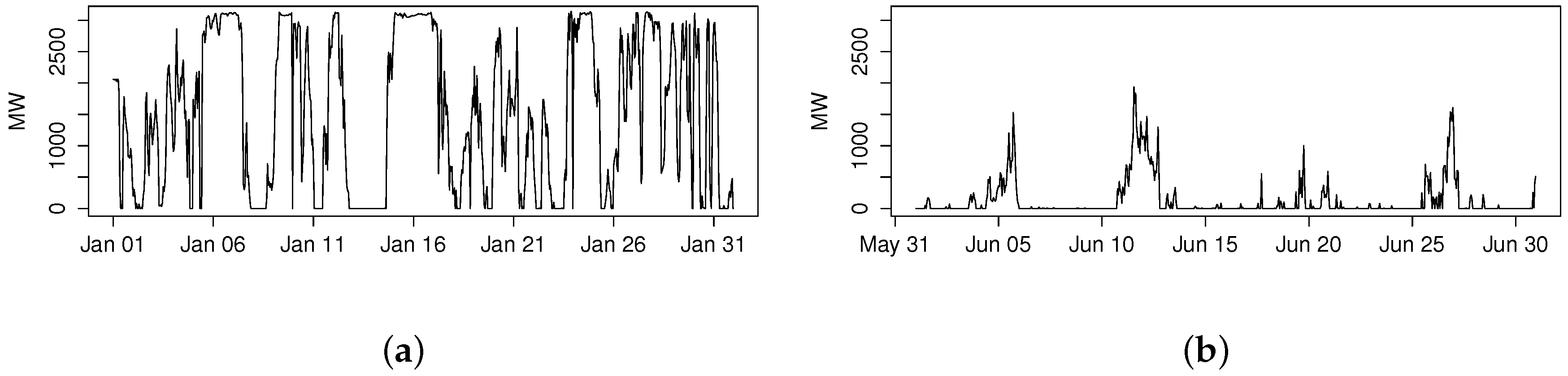
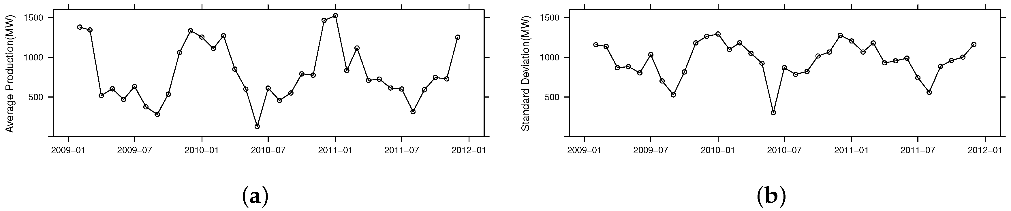
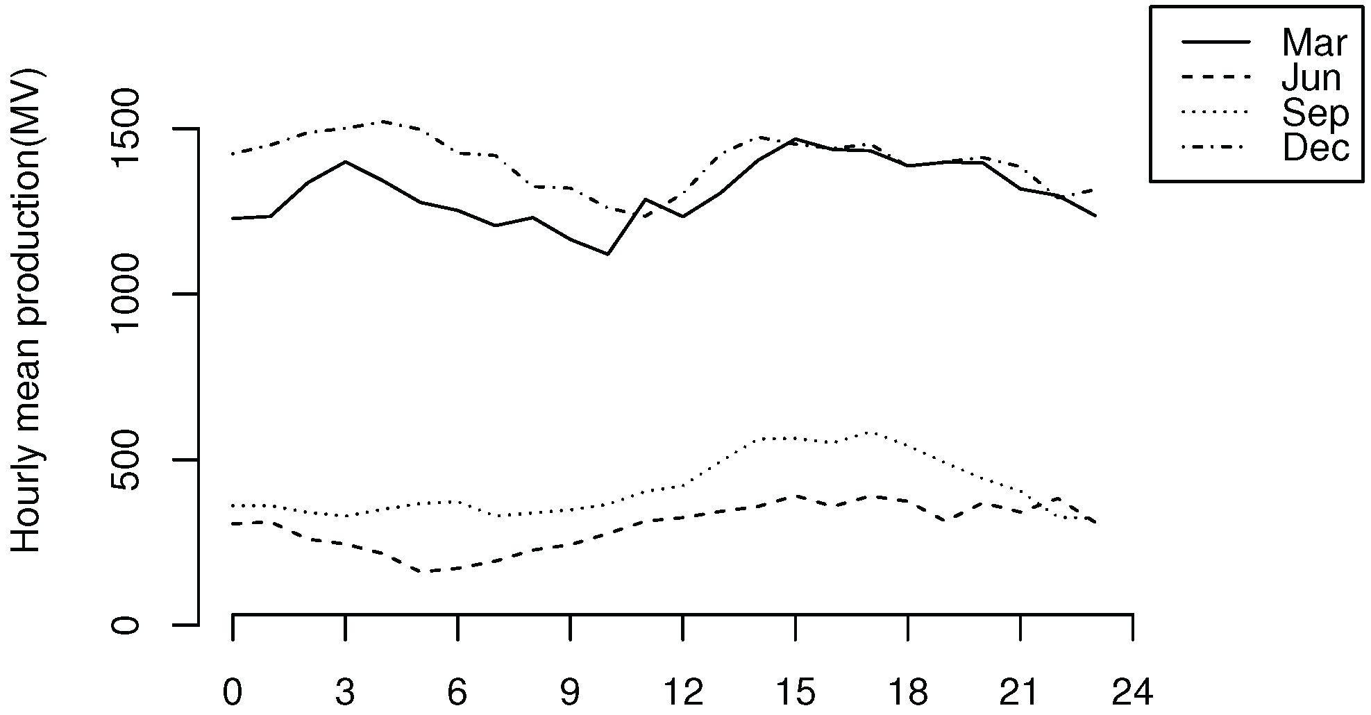
Figure 4 shows the wind electricity generated in January 2011 and June 2010, and indicates that the amount and variability of wind electricity are different for each month. The mean and standard deviation of each month are shown in Figure 5. As shown in these figures, the monthly difference is clearly observed. In Figure 6, the mean values of wind electricity per hour for each month are shown and hourly patterns seem obvious. Even though the yearly variation exists, it is not as significant as monthly and hourly variations. Thus, we focus on monthly and hourly variations to build a stochastic wind power model.

The wind electricity has often been modeled as an autoregressive (AR) model in the literature [24,35], so we extensively analyzed the collected data and found that the collected data can also be properly modeled by an AR model in our previous study [36]. The procedures for the data preprocessing and the model development can be summarized as follows. First, we transform the raw data, shown to be a non-stationary and non-Gaussian process, into the data, which follow a stationary and Gaussian process. Then, to remove the seasonal and diurnal effects of the transformed data, each of the data is standardized and stabilized by Equation (10), which is similar to standardizing normally distributed data:

$$\begin{array}{c}\hfill z_t=\frac{G(w_t)-G({\overline{w}}_t^{(m,h)})}{{\sigma }_t^{(m,h)}},\end{array}$$

(10)

where $w_t$ is the amount of wind electricity at time t, $G(·)$ is a transformation function such as the box-cox transformation, m is the index for month during a year (m = 1 … 12),

h is the index for one hour $[h,h+1)$ during a day (h = 0 … 23), and ${\overline{w}}_t^{(m,h)}$ and ${\sigma }_t^{(m,h)}$ are the sample mean and standard deviation of wind electricity generated at corresponding hour, h, on month, m. By testing several statistical tests, we conclude that the resulting $z_t$ with $G(·)=\sqrt{·}$ for the hourly data of two years can be effectively modeled by AR(1) as follows:

$$\begin{array}{c}\hfill z_t=\varphi z_{t-1}+ϵ,\end{array}$$

where $\varphi$ is the AR coefficient and $ϵ\sim N(0,{\sigma }_Z^2)$, which are estimated as $\varphi =0.9335$ and ${\sigma }_z^2=0.1265$ for our data.

To develop a discretized version of the dynamic programming for our MDP model, we discretize the wind electricity generation and construct the trinomial model for each month by the method described in Jaillet et al. [37]. In our numerical study, the trinomial lattice is built to model $z_t$ for two days each month, i.e., 48 h, to coordinate the analysis time horizon of our MDP model and the corresponding wind electricity, $w_t$, is obtained by reversing the Equation (10) and limiting each value between maximum (3 MW) and minimum values (0 MW). Here, since AR(1) is a discrete-time analogue of the mean-reverting process, the wind electricity model is basically a Markov process.

6.3. Electricity Price Model

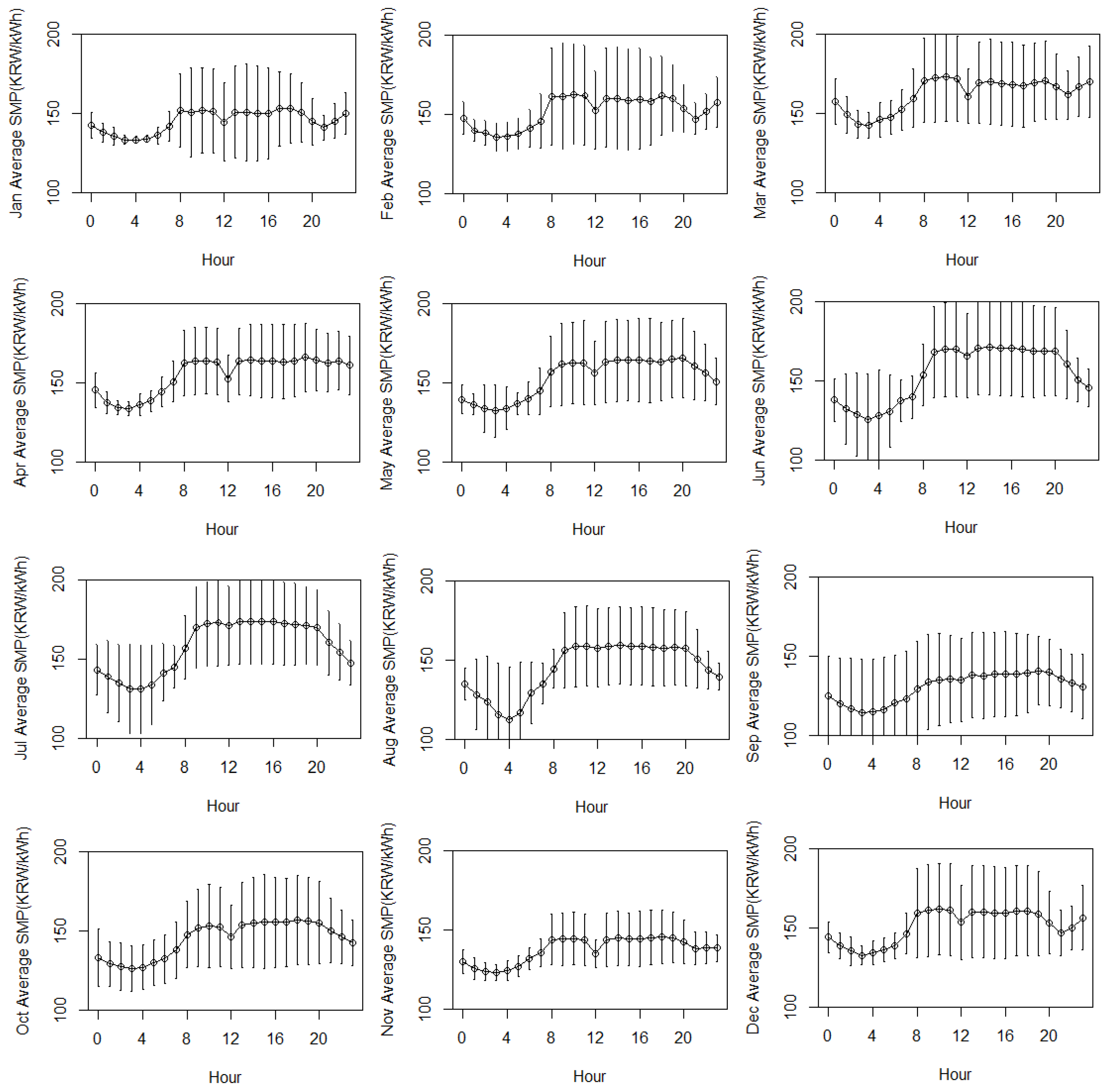
In a similar way to the method of constructing the wind electricity model, we collected historical data of electricity prices in the Korean electric power system, in order to construct the electricity price model. We collected hourly-based SMP data during the last three years, from 2012 to 2014, from a web-based database system operated by Korea Power Exchange, Electric Power Statistic Information System (EPSIS) [38]. The data exhibit the minimum and maximum SMPs during the years at 34.51 KRW/kWh and 281.76 KRW/kWh, respectively. Figure 7 shows the estimated average SMPs and its standard deviations at each h and each m, used for this numerical example.

By using the historical data, we develop an independent and identically distributed (IID) price model as in the literature [25]. It contains two main characteristics of electricity price—hourly and monthly seasonality as well as volatility, as follows:

$$\begin{array}{c}\hfill p_t={\overline{p}}_t^{(m,h)}+{\sigma }^{(m,h)}{e}_t,\end{array}$$

(11)

where ${\overline{p}}^{(m,h)}$ is the estimated sample mean SMP at corresponding h and m, ${\sigma }^{(m,h)}$ is the estimated sample standard deviation of SMPs at corresponding h and m, and $e_t$ is the IID standard normal random number ($e_t\sim$ $i.i.d.$ $N(0,1)$). By discretizing the random number $e_t$ into seven numbers with the probabilities from the standard normal distribution, we also discretize the electricity price model.

6.4. Costs and Capacities of the ESS

In order to find the optimal ESS size, the capital costs of ESS should be incorporated as we described in Section 5. Even though the ESS capital costs are still very uncertain, we use the reference capital costs based on recent, highly cited literature [39,40]. Among several types of storage technologies, we focus on the capital costs of the lithium-ion battery as our reference costs data in this numerical study, which are 600–2500 USD/kWh for storage capacity and 1200–4000 USD/kW for charging/discharging capacity. Even though it has higher costs compared to other technologies, we choose the technology because it has many advantages such as high energy density, high charge/discharge currents, and high efficiency, so it is the most popular in several recent real-world ESS projects in wind farms [2]. According to the projects, we further assume that its discharging duration time can vary from 15 min to 6 h, which is $0.25R\le S\le 6R$. In addition, we assume that the lifetime of the ESS is 10 years.

Using the reference costs of the lithium-ion battery, we simply calculate the equivalent annual cost (EAC) for $c_r$ and $c_s$ as follows:

$$\begin{array}{c}\hfill \mathrm{EAC}=\mathrm{Capital} \mathrm{Cost}\times \frac{0.1}{1-\frac{1}{{(1+0.1)}^{10}}}.\end{array}$$

(12)

The value ranges of $c_r$ and $c_s$ can be estimated as [195, 651] × ${10}^6$ KRW/MW/year and [98, 391] × ${10}^6$ KRW/MWh/year, respectively, when we assume that the exchange rate is 1000 KRW/$.

6.5. Results

6.5.1. Expected Annual Economic Value

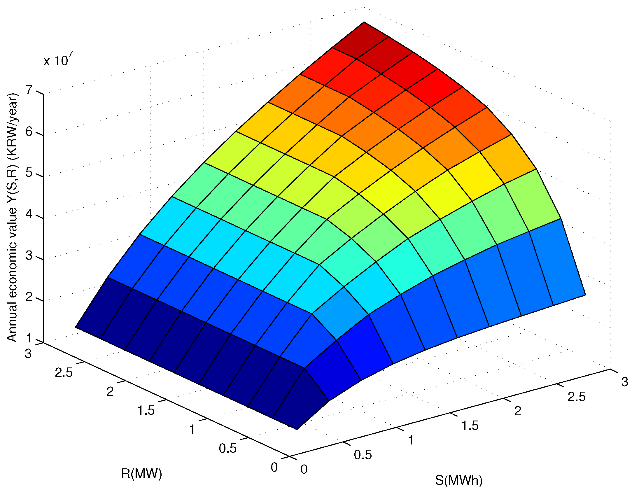
The results of numerical analysis show that the annual economic value of the ESS, $Y(S,R)$, depend on the sizes of storage capacity, S, and charging/discharging capacity, R. Figure 8 compares $Y(S,R)$ for different levels of S and R.

As expected, $Y(S,R)$ increases as the storage capacity and charging/discharging capacity increase, which indicates that storing more electricity and faster charging and discharging rates of ESS will give a better profit. However, the value $Y(S,R)$ does not increase in R when $R>S$, which implies that the charging/discharging capacity does not need to be greater than the storage capacity. Since the unit time period in this numerical study is one hour, the fast charging/discharging capability does not give an additional economic value for ESS—the charging/discharging capacity is large enough so the ESS can store or release electricity fully within one hour. It is also shown that $Y(S,R)$ is concave with respect to S and R, which means that the marginal value of $Y(S,R)$ decreases as R increases with a fixed S and as S increases with a fixed R.

We argue that the annual economic value of ESS largely depends on how to operate and manage the system, and the proposed MDP model is successful in achieving a better economic value by optimally operating the ESS. We validate the economic excellence of the proposed model by comparing the annual economic values obtained by applying two management policies for operating the ESS, one using the proposed MDP model and the other using a simple rule developed similar to the literature [13,16]. The simple rule uses the means of historical data of wind electricity and electricity price as their deterministic profiles, allows only one time of charge/discharge cycle per day, and makes the ESS fully charged at the lowest electricity price and fully discharged at the highest price.

For comparison purposes, we run a test for a situation where S and R are 1.5 MWh and 1.5 MW, respectively. The test shows that operating the ESS by the simple rule provides much lower economic value than using an optimal policy proposed in this study. The economic value based on the simple rule is approximately 17 $\times {10}^6$ KRW/year, which is only about 40% of the economic value expected from our method. This simple comparison strongly supports the importance of an optimal policy for operating the ESS. Furthermore, it implies that wind farm owners are likely to make an erroneous decision on the ESS size determination when they do not follow an optimal management policy but use a simple rule.

6.5.2. Optimal Size

With the above annual economic value of ESS, the optimal storage size $S^{\ast }$ and optimal charging/discharging capacity $R^{\ast }$ in Equation (8) can be obtained when the financial cost of storage ($c_{r}R+c_{s}S$) is specified. Given the cost ranges we refer to in Section 6.4, we surmise that it is impossible to make a profit from the ESS in the wind farm. We further note that, if the reference costs were reduced by a factor of 10, then the wind farm may make a profit from the installation of ESS with appropriate sizes of S and R. Therefore, we consider the revised reference costs (reduced by a factor of 10) below. To help select the optimal values of S and R, Figure 9 presents the expected annual economic value, $Y(S,R)$, and is compared with the cost range of $c_r$, [19.5, 65.1] $\times {10}^6$ KRW/MW/year, with different values of R for a fixed $S=1.5$ MWh ($c_s=10\times {10}^6$ KRW/MWh/year), which is a two-dimensional cross-section of the three-dimensional values in Figure 8. Even with the revised reference costs, the installation of ESS is not profitable in most cases. Nevertheless, by selecting R between $0.3$ MW and $1.5$ MW, the installation of ESS into the given wind farm can be profitable with the investment cost close to the lower bound (i.e., $c_c$ is close to 19.5 $\times {10}^6$ KRW/MW/year). In addition, notice that $Y(S,R)$ stays at the same value when R is greater than 1.5 MW because the storage size S is set to 1.5 MWh, which indicates that R does not have to be greater than S.

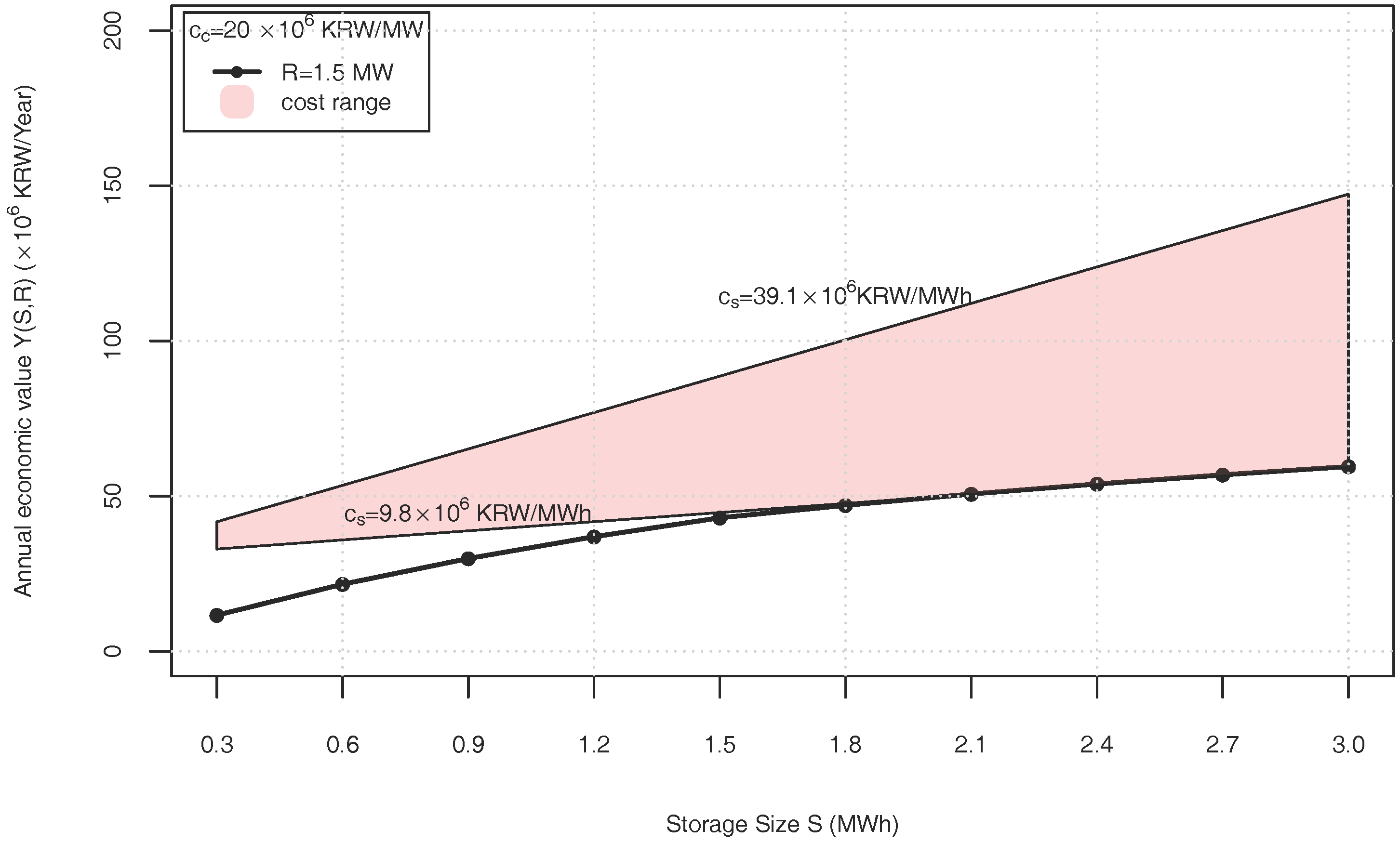
On the other hand, Figure 10 shows the expected annual economic value, $Y(S,R)$, and is compared to the cost range of $c_s$, [9.8, 39.1] $\times {10}^6$ KRW/MWh/year, with different values of S for a fixed $R=1.5$ MW ($c_r=20\times {10}^6$ KRW/MW/year), which is also a two-dimensional cross-section of Figure 8. Due to the high cost of R ($20\times {10}^6$KRW/MW/year), the profit cannot be earned until S is greater than about 1.8 MWh with the investment cost close to the lower bound (i.e., $c_s$ = 9.8 × ${10}^6$ KRW/MWh/year). To determine an appropriate choice of the ESS size, a careful comparison of $c_r$ and $c_s$ should be made to maximize the economic benefit from the ESS. From the results in Figure 9 and Figure 10, it can be seen that S needs to be at least greater than R and R needs to be greater than $S/5$, i.e., $R<S<5R$.

From the above comparisons between economic values of ESS and costs ranges, we establish a guideline for a wind farm owner who is considering the installation of the ESS, about how he or she can decide appropriate sizes of the ESS, S and R, in his or her farm. Furthermore, the comparison results give other guidelines to ESS manufacturers and policy makers. ESS manufacturers can identify how much they need to reduce costs of ESS in order for the ESS to have cost-competitiveness in South Korea, and, at the same time, the policy makers can identify how much subsidy the government needs to provide for the installation of the ESS in wind farms under the given electricity wholesale market, wind electricity potential, and costs of the ESS.

6.5.3. Sensitivity Analysis

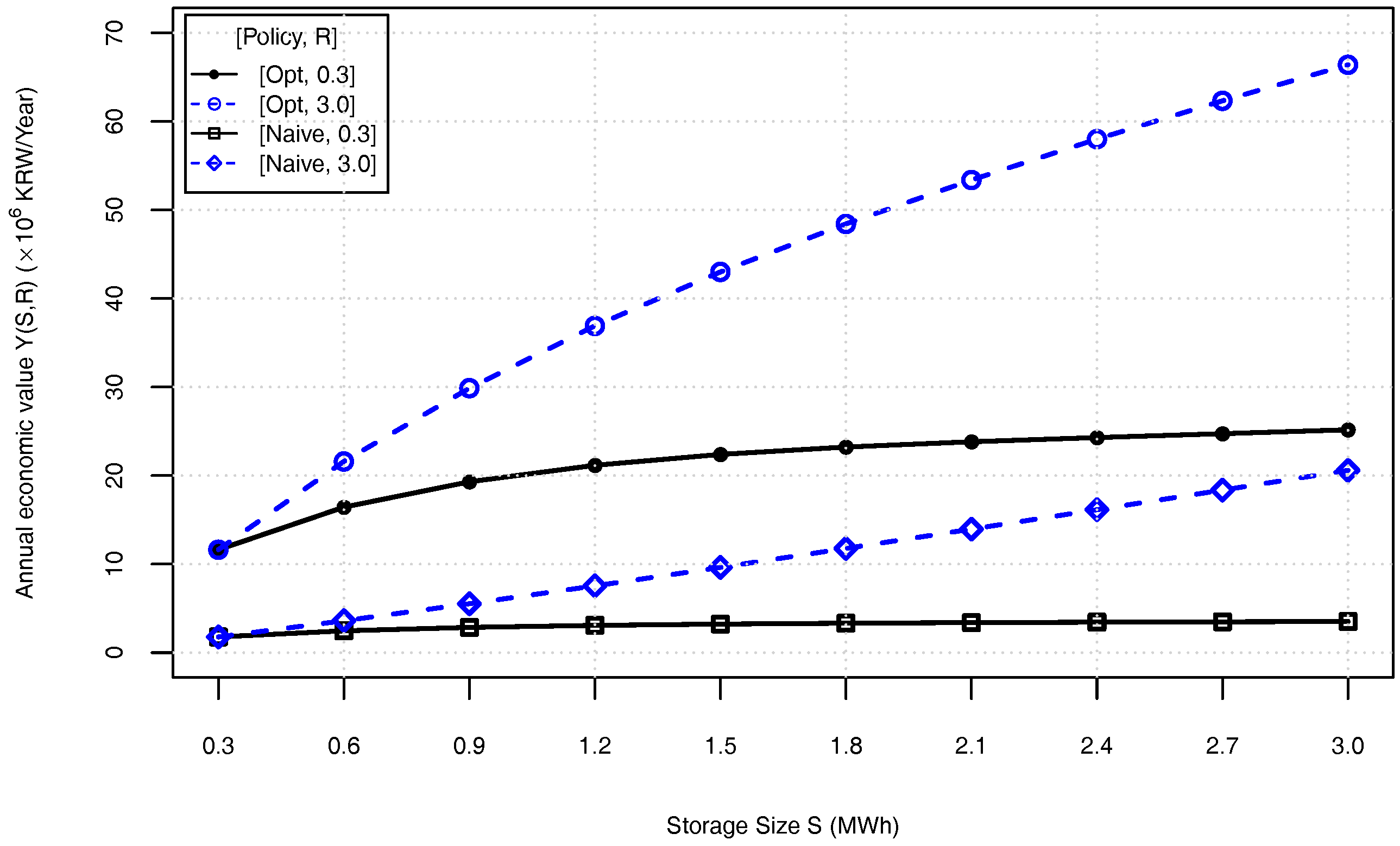
In our numerical study, we notice that the economic value of the ESS is affected by several factors such as ESS management policy, wind electricity variability, and electricity price variability. First of all, the management policy of the ESS can affect the economic value. Figure 11 illustrates the effect of the management policy. It shows the difference between the expected annual economic values of the ESS, $Y(S,R)$, under the optimal management policy and a naive management policy by varying the storage capacity size, S, with two charging/discharging capacity sizes of R, 0.3 MW and 3 MW.

The naive management policy is one of the simplest policies where the ESS is charged or discharged as much as possible if the current electricity price is the minimum or maximum in our price model, respectively, and do nothing otherwise. As shown in Figure 11, the differences of $Y(S,R)$ between two management policies are notably large with most combinations of S and R. Note that the marginal economic benefits from increasing the capacities of the ESS quickly drop to zero under the naive management policy. Thus, the economic gains obtained by the optimal management policy over the naive management policy increases as S and/or R increases. This result indicates that the choice of the ESS management policy is critical when the optimal ESS size is determined. Consequently, the benefit from ESS can be maximized not only with the optimal size of ESS and but also when the ESS management policy is carefully determined.

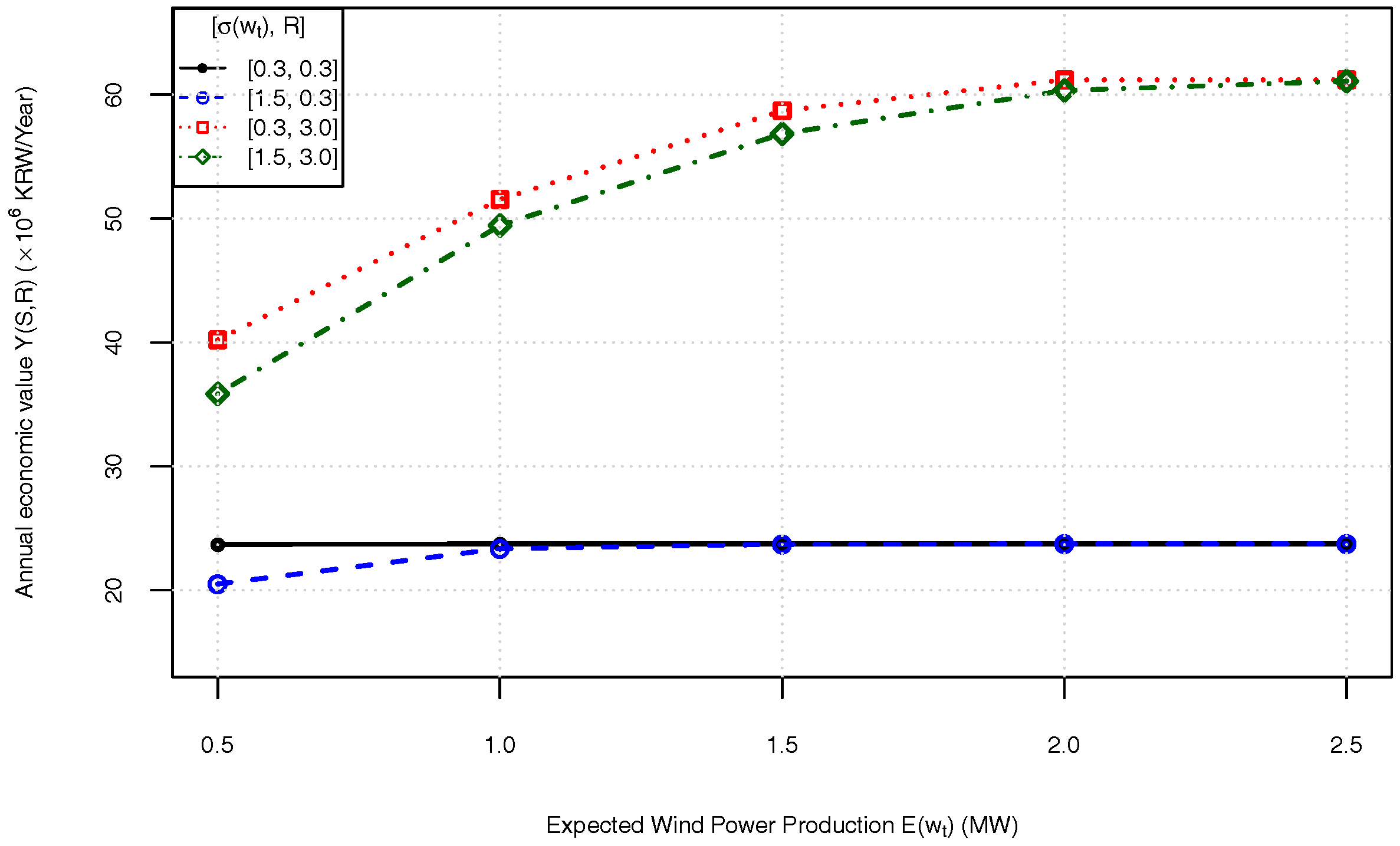
To see the impact of wind electricity variability, Figure 12 shows the expected annual economic values of the ESS, $Y(S,R)$, when the wind electricity model has a different mean and standard deviation. It shows the results when the storage capacity size, S, is set to 1.5 MWh and charging/discharging capacity sizes, R, are set to 0.3 MW or 3 MW.

To remove the monthly effect of $w_t$, we fix the mean and standard deviation of $w_t$, i.e., ${\overline{w}}_t^{(m,h)}$ and ${\sigma }_t^{(m,h)}$ in Equation (10). As a result, the trinomial model for $w_t$ becomes the same for each month. With 3 MW of R, the $Y(S,R)$ increases as more $w_t$ is produced, but when the mean of $w_t$ is greater than the storage capacity size $S=1.5$ MWh, the increment of $Y(S,R)$ becomes smaller, as expected. It is interesting to note that the larger variability of $w_t$ does not help improve the economic benefit of the ESS. This is because a larger variability of $w_t$ might give less of a chance to take advantage of the price variability, compared to a smaller variability of $w_t$, i.e., it would be unable to charge more at a lower price and discharge more at a higher price. With 0.3 MW of R, the distribution of $w_t$ does not affect $Y(S,R)$ much since the use of the ESS is limited due to the small value of R.

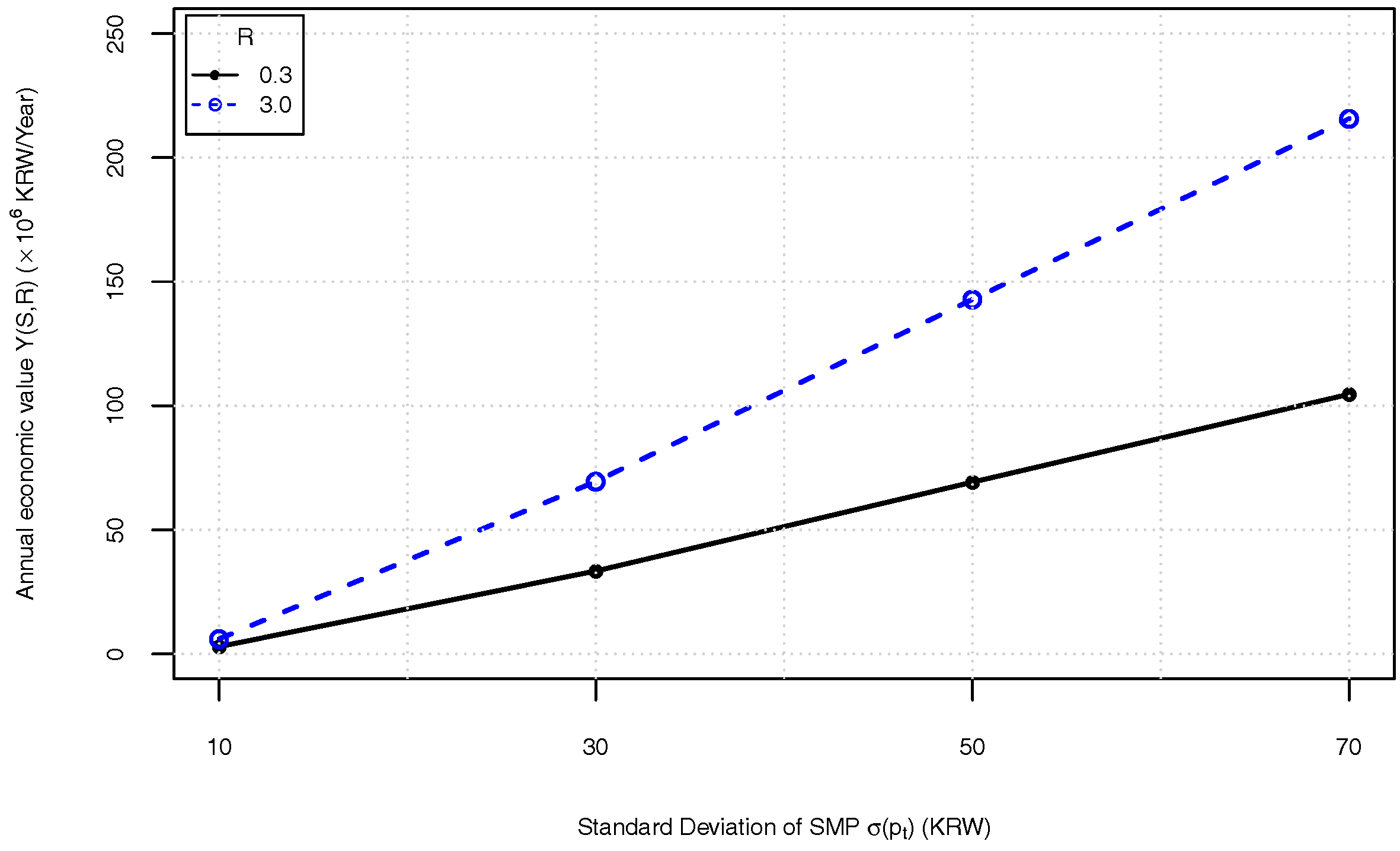
Lastly, Figure 13 compares the expected annual economic values of the ESS, $Y(S,R)$, when the electricity price model has a different standard deviation with a fixed mean, ${\overline{p}}_t^{(m,h)}=150$ KRW/kWh. It also shows results when the storage capacity size, S, is set to 1.5 MWh and charging/discharging capacity sizes, R, are set to 0.3 MW or 3 MW. To remove the monthly effect of $p_t$, we fix the mean and variance of $p_t$ for each month and each hour in Equation (11). We should note that a larger variability of $p_t$ improves the economic benefit of the ESS because the electricity range becomes wider with the larger variance of $p_t$.

7. Conclusions

This paper describes how to identify the optimal management policy of the ESS installed in a grid-connected wind farm in terms of maximizing economic benefits, and, more importantly, provides an analytic guideline for defining the economic value of ESS under the policy and selecting its optimal size. Furthermore, a numerical study is carried out to show its usefulness.

In this paper, we define the economic value of ESS as the difference between the average profit made by selling electricity from a wind farm with ESS and one without ESS, and prove that the economic value of ESS is non-decreasing and jointly concave with respect to the storage capacity and charging/discharging capacity sizes. By the numerical results, we show that the economic value of ESS increases but its marginal increment decreases as the size of ESS increases. In addition, we find that the economic value of ESS can be affected by the management policy, wind electricity variability, and electricity price variability. This result implies that, even with specific investment costs of ESS, the optimal size of ESS can vary depending on the locational characteristics (about wind electricity and electricity price) and the management policy of the wind farm, so there is no specific solution for the optimal size of ESS. Hence, this study could help the wind farm owners, who are considering the installation of the ESS, make their decisions.

We find that the current investment cost level of the ESS is too high to make a profit by its use, but battery technology has been growing rapidly, driven by the popularity of electric vehicles and renewable energies. Therefore, its costs are expected to decrease significantly in a few years, and then this study will become more valuable. Furthermore, even though we have evaluated the value of the ESS in terms of economic perspective, ESS is, in practice, also utilized for other objectives such as wind power quality and reliable electricity supply. Thus, it would be interesting to expand this study to find the optimal ESS size considering multi-objectives.

The analysis of this paper is based on the assumption that the uncertain variables such as the wind power generation and the electricity price value evolve according to discretized models. Although the optimal policy can be effectively found by our MDP model, the discretization error from modeling those uncertain variables could lead to suboptimal results. This will be the subject of our future research.

References

- IEA. World Energy Outlook 2015; Technical Report; IEA: Paris, France, 2015. [Google Scholar]
- U.S. Department of Energy. Energy Storage Database. Available online: http://www.energystorageexchange.org/ (accessed on 7 March 2018).
- Ministry of Trade, Industry and Energy. 4th Renewable Energy Basic Plan (in Korean), 2014. Available online: http://www.motie.go.kr/motie/py/td/Industry/bbs/bbsView.do?bbs_cd_n=72&cate_n=1&bbs_seq_n=210142 (accessed on 7 March 2018).
- Wade, N.; Taylor, P.; Lang, P.; Jones, P. Evaluating the benefits of an electrical energy storage system in a future smart grid. Energy Policy 2010, 38, 7180–7188. [Google Scholar] [CrossRef] [Green Version]
- Zhu, D.; Wang, Y.; Yue, S.; Xie, Q.; Pedram, M.; Chang, N. Maximizing return on investment of a grid-connected hybrid electrical energy storage system. In Proceedings of the 18th Asia and South Pacific Design Automation Conference (ASP-DAC), Yokohama, Japan, 22–25 January 2013; pp. 638–643. [Google Scholar]
- Bradbury, K.; Pratson, L.; Patiño-Echeverri, D. Economic viability of energy storage systems based on price arbitrage potential in real-time U.S. electricity markets. Appl. Energy 2014, 114, 512–519. [Google Scholar] [CrossRef]
- Walawalkar, R.; Apt, J. Market Analysis of Emerging Electric Energy Storage Systems (DOE/NETL-2008/1330); Technical Report; National Energy Technology Laboratory: Morgantown, WV, USA, 2008.
- Secomandi, N. Optimal Commodity Trading with a Capacitated Storage Asset. Oper. Res. 2010, 56, 449–467. [Google Scholar] [CrossRef]
- Charnes, A.; Dreze, J.; Miller, M. Decision and Horizon Rules for Stochastic Planning Problems: A Linear Example. Econometrica 1966, 34, 307–330. [Google Scholar] [CrossRef]
- Federgruen, A.; Zipkin, P.H. An Inventory Model with Limited Production Capacity and Uncertain Demands II. The Discounted-Cost Criterion. Math. Oper. Res. 1986, 11, 208–215. [Google Scholar] [CrossRef]
- Kapuscinski, R.; Tayur, S. A Capacitated Production-Inventory Model with Periodic Demand. Oper. Res. 1998, 46, 899–911. [Google Scholar] [CrossRef]
- Abhinav, R.; Pindoriya, N.M. Grid Integration of Wind Turbine and Battery Energy Storage System: Review and Key Challenges. In Proceedings of the 2016 IEEE 6th International Conference on Power Systems (ICPS), New Delhi, India, 4–6 March 2016; pp. 1–6. [Google Scholar]
- Berrada, A.; Loudiyi, K. Operation, sizing, and economic evaluation of storage for solar and wind power plants. Renew. Sustain. Energy Rev. 2016, 59, 1117–1129. [Google Scholar] [CrossRef]
- Denholm, P.; Sioshansi, R. The value of compressed air energy storage with wind in transmission-constrained electric power systems. Energy Policy 2009, 37, 3149–3158. [Google Scholar] [CrossRef]
- Fertig, E.; Apt, J. Economics of compressed air energy stroage to integrate wind power: A case study in ERCOT. Energy Policy 2011, 39, 2330–2342. [Google Scholar] [CrossRef]
- Johnson, J.X.; Kleine, R.D.; Keoleian, G.A. Assessment of energy storage for transmission-constrained wind. Appl. Energy 2014, 124, 377–388. [Google Scholar] [CrossRef]
- Korpaas, M.; Holen, A.T.; Hildrum, R. Operations and sizing of energy storage for wind power plants in a market system. Electr. Power Energy Syst. 2003, 25, 599–606. [Google Scholar] [CrossRef]
- Brekken, T.K.; Yokochi, A.; von Jouanne, A.; Hapke, H.M.; Yen, Z.Z.; Halamay, D.A. Optimal Energy Storage Sizing and Control for Wind Power Applications. IEEE Trans. Sustain. Energy 2011, 2, 69–77. [Google Scholar] [CrossRef]
- Zhang, L.; Li, Y. Optimal Energy Management of Wind-Battery Hybrid Power System with Two-Scale Dynamic Programming. IEEE Trans. Sustain. Energy 2013, 4, 765–773. [Google Scholar] [CrossRef]
- Luo, F.; Meng, K.; Dong, Z.Y.; Zheng, Y.; Chen, Y.; Wong, K.P. Coordinated Operational Planning for Wind Farm with Battery Energy Storage System. IEEE Trans. Sustain. Energy 2015, 6, 253–262. [Google Scholar] [CrossRef]
- Bridier, L.; Hernandez-Torres, D.; David, M.; Laurent, P. A heuristic approach for optimal sizing of ESS coupled with intermittent renewable sources systems. Renew. Energy 2016, 91, 155–165. [Google Scholar] [CrossRef]
- Shu, Z.; Jirutitijaroen, P. Optimal Operation Strategy of Energy Storage System for Grid-Connected Wind Power Plants. IEEE Trans. Sustain. Energy 2014, 5, 190–199. [Google Scholar] [CrossRef]
- Kim, J.H.; Powell, W.B. Optimal energy commitments with storage and intermittent supply. Oper. Res. 2011, 59, 1347–1360. [Google Scholar] [CrossRef]
- Zhou, Y.; Scheller-Wolf, A.; Secomandi, N.; Smith, S. Managing Wind-based Electricity Generation in the Presence of Storage and Transmission Capacity. Available online: http://ssrn.com/abstract=1962414 (accessed on 7 March 2018).
- Harsha, P.; Dahleh, M. Optimal Management and Sizing of Energy Storage Under Dynamic Pricing for the Efficient Integration of Renewable Energy. IEEE Trans. Power Syst. 2015, 30, 1164–1182. [Google Scholar] [CrossRef]
- Korea Energy Agency. Renewable Portfolio Standards(RPS). Available online: http://www.energy.or.kr (accessed on 7 March 2018).
- Go, R.S.; Munoz, F.D.; Watson, J.P. Assessing the economic value of co-optimized grid-scale energy storage investments in supporting high renewable portfolio standards. Appl. Energy 2016, 183, 902–913. [Google Scholar] [CrossRef]
- Lee, D.S.; Kim, S.N.; Choi, Y.C.; Baek, B.S.; Hur, J.S. Development of Wind Power Stabilization System using BESS and STATCOM. In Proceedings of the 2012 3rd IEEE PES Innovative Smart Grid Technologies Europe (ISGT Europe), Berlin, Germany, 14–17 October 2012; pp. 1–5. [Google Scholar]
- Kang, M.S.; Jin, K.M.; Kim, E.H.; Oh, S.B.; Lee, J.M. A study on the determining ESS capacity for stabilizing power output of Haeng-won wind farm in Jeju. J. Korean Sol. Energy Soc. 2012, 32, 25–35. [Google Scholar] [CrossRef]
- Nguyen, C.L.; Lee, H.H.; Chun, T.W. Cost-Optimized Battery Capacity and Short-Term Power Dispatch Control for Wind Farm. IEEE Trans. Ind. Appl. 2015, 51, 595–606. [Google Scholar] [CrossRef]
- Lim, J.H. Optimal Combination and Sizing of a New and Renewable Hybrid Generation System. Int. J. Future Gener. Commun. Netw. 2012, 5, 43–59. [Google Scholar]
- Cho, K.H.; Seul-Ki Kim, E.S.K. Optimal Capacity Determination Method of Battery Energy Storage System for Demand Management of Electricity Consumer. Trans. Korean Inst. Electr. Eng. 2013, 62, 21–28. [Google Scholar] [CrossRef]
- Wang, X.; Vilathgamuwa, D.M.; Choi, S. Determination of Battery Storage Capacity in Energy Buffer for Wind Farm. IEEE Trans. Energy Convers. 2008, 23, 868–877. [Google Scholar] [CrossRef]
- United Nations Framework Convention on Climate Change. Project 3110: 3 MW Shinan Wind Power Project. Available online: https://cdm.unfccc.int/Projects/DB/KEMCO1257125689.44/view (accessed on 7 March 2018).
- Chen, P.; Pedersen, T.; Bak-Jensen, B.; Chen, Z. ARIMA-Based Time Series Model of Stochastic Wind Power Generation. IEEE Trans. Power Syst. 2010, 25, 667–676. [Google Scholar] [CrossRef]
- Ryu, J.H.; Choi, D.G. Development of a Stochastic Model for Wind Power Production. Korean Manag. Sci. Rev. 2016, 33, 35–47. [Google Scholar] [CrossRef]
- Jaillet, P.; Ronn, E.I.; Tompaidis, S. Valuation of Commodity-Based Swing Options. Manag. Sci. 2004, 50, 909–921. [Google Scholar] [CrossRef]
- Korea Power Exchange. Electric Power System Information System. Available online: https://epsis.kpx.or.kr/ (accessed on 7 March 2018).
- Zhao, H.; Wu, Q.; Hu, S.; Xu, H.; Rasmussen, C.N. Review of energy storage system for wind power integration support. Appl. Energy 2015, 137, 545–553. [Google Scholar] [CrossRef]
- Díaz-González, F.; Sumper, A.; Gomis-Bellmunt, O.; Villafáfila-Robles, R. A review of energy storage technologies for wind power applications. Renew. Sustain. Energy Rev. 2012, 16, 2154–2171. [Google Scholar] [CrossRef]
- Porteus, E. Foundations of Stochastic Inventory Theory; Business/Marketing, Stanford University Press: Stanford, CA, USA, 2002. [Google Scholar]
Figure 1.
System definition.
Figure 2.
Cases of two state variables and .
Figure 3.
The structure of optimal charging/discharging action of the ESS in the case 3, .
Figure 4.
Wind electricity generation of the wind farm in Shinan, South Korea. (a) wind electricity on January 2011; (b) wind electricity on June 2010.
Figure 5.
Monthly statistics of wind electricity of the wind farm in Shinan, South Korea. (a) average wind electricity; (b) standard deviation of wind electricity.
Figure 6.
Average wind electricity generation per hour for each month.
Figure 7.
Estimated sample mean and one standard deviation range of SMPs at each hour on each month based on 3-year historical data in the Korean electric power system.
Figure 8.
Annual economic values for different storage sizes S and different charging/discharging capacities R.
Figure 9.
Annual economic values for different values of R and the range of unit cost per year when MWh and KRW/MWh/year.
Figure 10.
Annual economic values for different storage sizes and the range of unit cost per year when MW and KRW/MW.
Figure 11.
Annual economic values of the optimal policy vs. that of the naive policy with different storage capacity size.
Figure 12.
Annual economic values for different mean and standard deviations of wind electricity model, and . ( MWh).
Figure 13.
Annual economic values for different standard deviations of SMP ( = 150 KRW/kWh).