Wave Resource Characterization Using an Unstructured Grid Modeling Approach

Abstract

This paper presents a modeling study conducted on the central Oregon coast for wave resource characterization, using the unstructured grid Simulating WAve Nearshore (SWAN) model coupled with a nested grid WAVEWATCH III^® (WWIII) model. The flexibility of models with various spatial resolutions and the effects of open boundary conditions simulated by a nested grid WWIII model with different physics packages were evaluated. The model results demonstrate the advantage of the unstructured grid-modeling approach for flexible model resolution and good model skills in simulating the six wave resource parameters recommended by the International Electrotechnical Commission in comparison to the observed data in Year 2009 at National Data Buoy Center Buoy 46050. Notably, spectral analysis indicates that the ST4 physics package improves upon the ST2 physics package’s ability to predict wave power density for large waves, which is important for wave resource assessment, load calculation of devices, and risk management. In addition, bivariate distributions show that the simulated sea state of maximum occurrence with the ST4 physics package matched the observed data better than with the ST2 physics package. This study demonstrated that the unstructured grid wave modeling approach, driven by regional nested grid WWIII outputs along with the ST4 physics package, can efficiently provide accurate wave hindcasts to support wave resource characterization. Our study also suggests that wind effects need to be considered if the dimension of the model domain is greater than approximately 100 km, or O (10² km).

1. Introduction

Third-generation wave models have been significantly developed in recent years to capture nonlinear wave–wave interaction dynamics and nearshore shallow water hydrodynamics. The most popular third-generation phase-average spectral models, such as WAVEWATCH III^® (WWIII) [1], the Wave Action Model (WAM) [2], Simulating WAve Nearshore (SWAN) [3], TOMAWAC [4], and MIKE-21 Spectral Wave (MIKE-21 SW) [5] models, have been widely validated in many coastal waters and open oceans worldwide. For example, the WWIII model has been maintained and used for operational ocean wave forecasts by the National Oceanic and Atmospheric Administration’s (NOAA’s) National Centers for Environmental Prediction (NCEP) [1,6,7]. The WAM is operated by the European Centre for Medium-Range Weather Forecasts (ECMWF), which provides wave hindcast data over the North Atlantic Ocean. WWIII results have been used to produce the first ocean wave energy resource assessment in the United States [8]. The WAM was also used to estimate wave energy resources in Europe. Both the WAM and WWIII are most commonly used to simulate wind-generated waves in deep waters and provide open boundary conditions for simulating wave dynamics in intermediate and shallow water areas. WWIII uses a time-splitting approach, calculating the solution of the energy balance equation differing from the WAM’s numerical scheme [9]. Although WWIII includes curvilinear, structured, and unstructured grid options, the structured grid has been the most commonly used.

In contrast to structured grid models, unstructured grid models use flexible meshes that have high resolutions to represent the complicated bottom topography and irregular coastlines in nearshore areas (coarser resolutions are used for other areas). Hence, it is computationally more efficient to simulate wave climate with high spatial variability using one model grid without nesting [10]. For instance, TOMAWAC, a third-generation spectral wave model within the integrated TELEMAC modeling system, uses the finite element numerical method in an unstructured grid framework [11]. The TELEMAC system was originally developed by the Laboratoire National d’Hydraulique et Environnement in France and its primary users are based in European countries. UnSWAN is the unstructured grid version of the SWAN wave model, which has been widely used worldwide [10,12,13,14]. Please note that “unstructured grid SWAN” is often used in the literature, but that for the sake of brevity we shall use “UnSWAN” in this paper.

The main benefit of unstructured grids is that they can be applied at variable spatial resolutions while using the same flexible computational grid. Flexible meshes are useful in capturing the sharp gradients at varying water depths. MIKE 21 SW is the commercial 3G spectral wave sub-module of the MIKE 21 modeling system that solves action balance equations on an unstructured grid, using a finite volume method [15]. Similar to UnSWAN, it simulates the effects of various nonlinear physical effects. A recently developed unstructured grid version of WWIII remains under continuous development and validation [1,16,17,18,19]. Because the development of unstructured grid spectral wave models is relatively new compared to that of structured grid models, previous applications of unstructured grid wave models to characterize wave climate and resources are limited. Recently, Robertson et al. [20] applied UnSWAN to simulate wave resource characterization on the Pacific Northwest coast of Vancouver Island, British Columbia, which has very complex coastlines and a narrow continental shelf. Based on a review of the literature, we found that the UnSWAN is more popular and better validated than other unstructured grid wave models, including TOMAWAC, unstructured grid WWIII, and MIKE-21 SW. Therefore, UnSWAN was selected for this study because of its sophistication and popularity.

The International Electrotechnical Commission (IEC) released a Technical Specification (TS) for wave energy resource assessment and characterization that includes a set of standards and methods for consistent and accurate assessment of wave energy resources [21]. Following IEC TS recommendations, a number of wave energy resource assessment studies have been conducted. Lenee-Bluhm et al. assessed and characterized the wave energy resource of the U.S. Pacific Northwest using six characteristic quantities, compared with the archived spectral records from 10 wave measurement buoys from the National Data Buoy Center (NDBC) and the Coastal Data Information Program (CDIP) [22]. Akpinar et al. presented a potential wave energy assessment in the Black Sea and showed spatial distribution maps based on monthly, seasonal, and annual averages for the establishment and design of a wave energy converter (WEC) system [23]. García-Medina et al. conducted a seven-year hindcast, using nested grid WWIII and structured grid SWAN models to assess the temporal and spatial variability as well as the trend of wave resources in Oregon and southwestern Washington [24,25]. Yang et al. conducted a wave resource assessment at a test bed off the central Oregon coast, using structured grid WWIII and SWAN with a four-level nested grid approach. The physics packages were also compared to better understand the effects of the ST4 physics model for predicting wave characteristics in the frequency and directional 2D domain [26]. Structured grid WWIII and SWAN were used to evaluate wave energy resources on the United Kingdom’s southwest coast and on France’s west coast by Soares et al. and Goncalves et al. They found that the model performance of simulating significant wave height is better than that of mean period [27,28]. Silva et al. used WWIII and SWAN to assess wave energy resources with high resolution. They identified the differences in wave energy resources between the Iberian north and west coast with the consistent parameterization of the SWAN model setup and wind forcing [29]. Bento et al. assessed potential wave energy resources at Galway Bay using WWIII and SWAN. They found that the model performance was not good in the bay, because it is difficult for the model to generate local wind waves in a small fetch within the enclosed bay area [30]. Morim et al. assessed the wave energy resource along the southeastern coast of Australia, using the structured grid WWIII and the curvilinear SWAN. They indicated that the wind field observations from the coastal ocean to overland wind would be considered for the future research [31]. Akpinar et al. recommended applying unstructured grid systems and validating wind fields against observed wind data to further improve the wave model [32].

This paper describes how the model skills of WWIII and UnSWAN for predicting the wave energy resource parameters recommended by the IEC TS were calculated and compared with those calculated from the WWIII results. Because wave models and the quality of wave hindcasts are highly dependent on the quality of the wind field [32,33,34,35], the sensitivity of wind effects on wave predictions was also investigated. A detailed validation of physics packages using the modeled wave spectra and bivariate distributions is described.

2. Methods

2.1. Wave Models

Both WWIII and UnSWAN were used in this study. UnSWAN includes source terms for linear and exponential wind input growth and the formulation for wind input parameterization. Dissipation terms due to whitecapping, depth-induced wave breaking, and quadruplet and triad wave interactions were considered in the simulation. WWIII consists of source terms with different physics package options that consider sea ice and various wind–wave interaction and dissipation effects [6,36,37]. Specifically, the ST2 physics package is based on previously developed wind input and nonlinear interaction source terms and a new dissipation source term consisting of high- and low-frequency constituents [36]. The ST4 physics package consists of new parameterizations for swell, wave breaking, and short-wave dissipations of winds-generated waves, which are consistent under a wide range of conditions and at scales from the global ocean to coastal regions [37]. Both ST2 and ST4 physics packages were evaluated in this study.

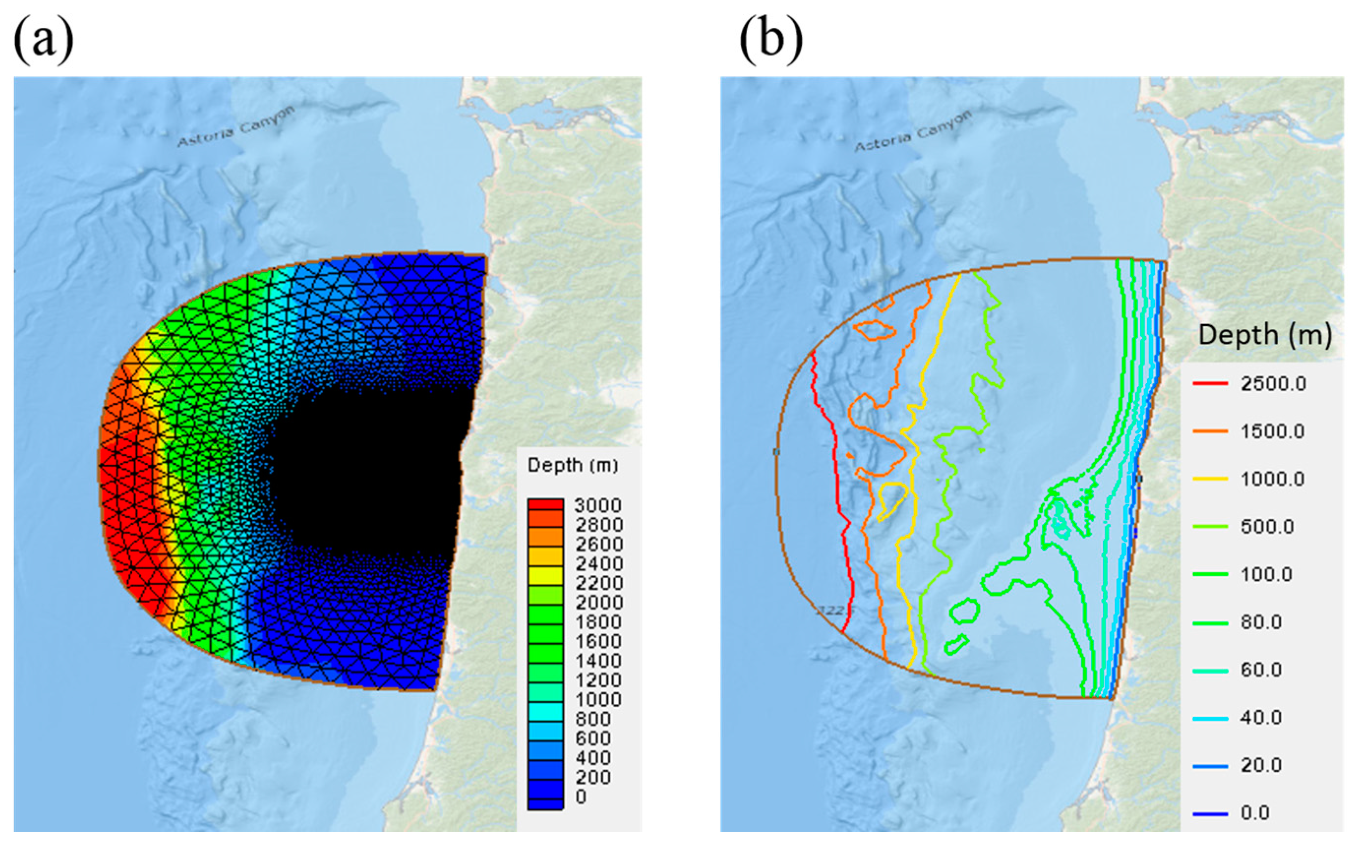
2.2. Wave Model Grids

The model domain chosen off the central Oregon coast is shown in Figure 1. Real-time wave and meteorological data were collected from NDBC Buoy 46050 inside the model domain, using representative water depth and high-quality, long-term wave measurements.

A nested grid modeling approach was employed to drive the UnSWAN model in this study. Three levels of structured grid WWIII models provide the open boundaries for the unstructured grid model. The model domain coverage, spatial resolution, and grid size (number of grid points) for Global Grid L1 and two Intermediate Grids L2 and L3, are summarized in

Table 1. Grid information for WAVEWATCH III^® (WWIII).

Grid Name	Coverage	Resolution (Long., Lat.)	Grid Size
Global Grid L1	77.5° S–77.5° N	0.5° × 0.5° (30′ × 30′)	223,920
Intermediate Grid L2	35°–50° N; 128°–120° W	0.1° × 0.1° (6′ × 6′)	12,231
Intermediate Grid L3	43.6°–45.9° N; 125.6°–123.8° W	1′ × 1′	15,151

. The model output from the Intermediate Grid L3 provides wave open boundary conditions for the unstructured grid model domain.

The model bathymetry for all grid levels was interpolated using three NOAA bathymetry data sets: (1) 1 arc-minute ETOPO1 Global Relief Model, (2) 3 arc-second Coastal Relief Model, and (3) 1/3 arc-second tsunami high-resolution bathymetry data. The 1 arcminute ETOPO1 Global Relief Model was used for the outer shelf region and the deep ocean basins. The 3 arcsecond (~90 m) Coastal Relief Model for the inner shelf region was used for the model bathymetry and for the L2 to UnSWAN model domain. The resolution of the Coastal Relief Model data set was sufficient for the inner shelf region, because the local model grid resolution is approximately 300 m. The model bathymetry was further interpolated from NOAA’s high-resolution (1/3 arcsecond) tsunami bathymetry data. The dimension of the unstructured grid for the model domain is 12 arcsec by 10 arcsec. The unstructured grid of the model domain includes 44,974 nodes and 89,100 elements.

An extended UnSWAN model grid, UnSWAN (L), was generated to support the conduct of additional sensitivity tests of unstructured grid flexibility and wind effect. UnSWAN (L) covers a much larger region with flexible meshes―from approximately 125.6° W to 124° W in the longitudinal direction and from 43.7° N to 45.6° N in the latitudinal direction―to demonstrate the flexibility and efficiency of unstructured grid models. The UnSWAN (L) model grid and the bathymetric features are shown in Figure 2. For the internal region that overlays the UnSWAN model domain (water depth less than 500 m), the grid resolution is very fine and has an average element area of 82,066 m², which is equivalent to a side length of 435 m for an equilateral triangle. Outside the UnSWAN domain, the grid resolution gradually decreases to about 8000 m toward the open boundary, where the maximum water depth is about 3000 m (Figure 2).

2.3. Wave Model Forcing

Sea surface wind forcing is an important factor for accurately simulating wave growth, propagation, and dissipation. In this study, hourly wind vectors from the Climate Forecast System Reanalysis (CFSR) product were interpolated onto the UnSWAN model grid. The CFSR data use temporal intervals of 1 h and a resolution of 0.5 degree, which roughly meets the requirements of the IEC standards for wind forcing resolution (50 km) for feasibility class.

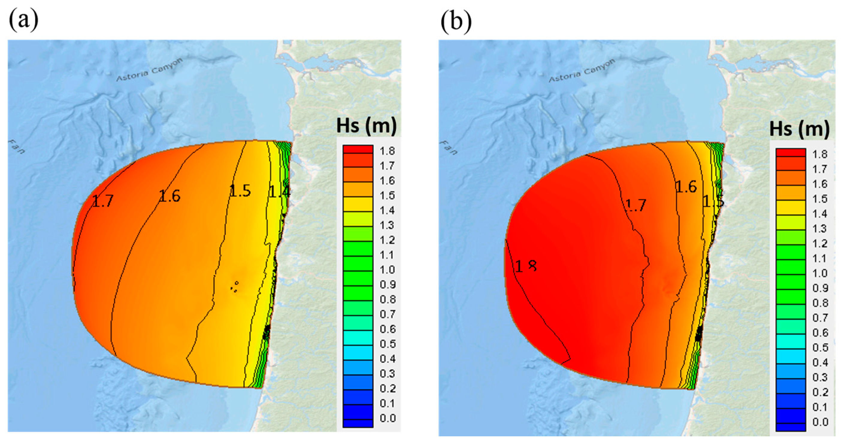
3. Results and Discussion

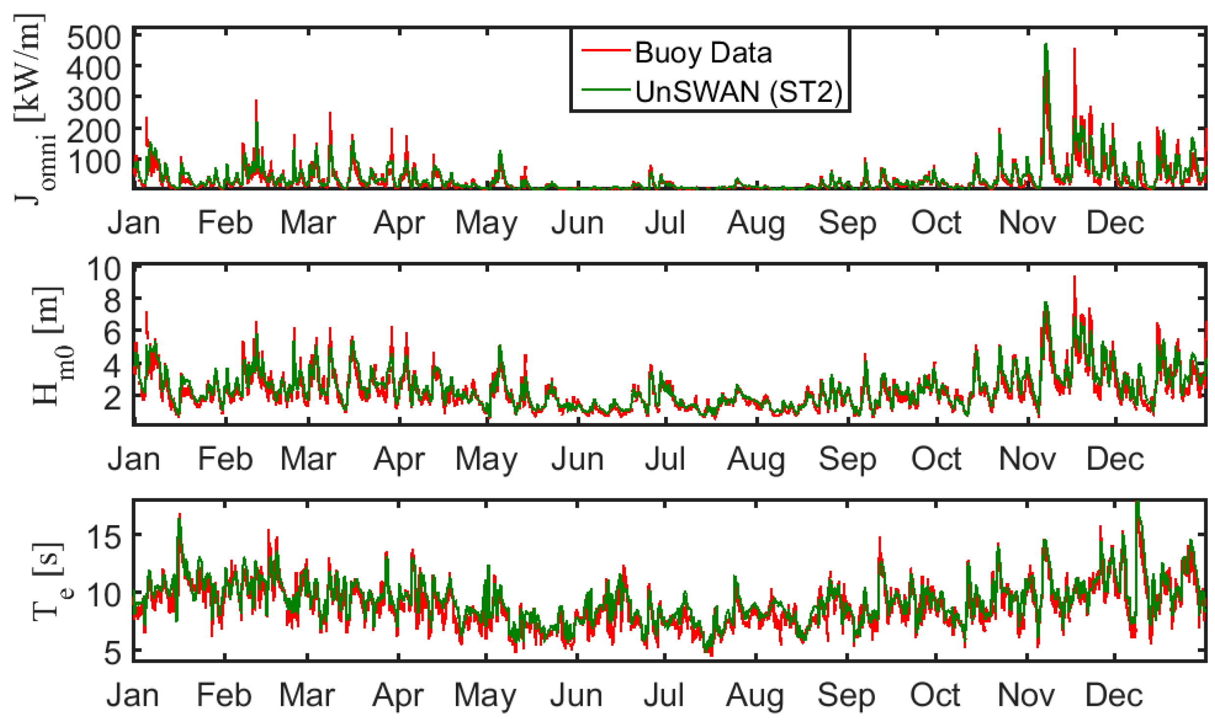
3.1. Model Simulations

UnSWAN was applied to all model simulations in this study by using the non-stationary mode with spherical coordinates. The model configuration uses 29 spectral frequency bins ranging from 0.035 to 0.505 Hz with a logarithmic increment factor of 1.1, and 24 directional bins with a resolution of 15 degrees. This spectral resolution meets the minimum requirements specified by the IEC TS [21]: a minimum of 25 frequency components, 24 to 48 directional components, and a frequency range covering at least 0.04 to 0.5 Hz. The same spectral and directional resolutions were used in the WWIII model configuration. Default parameter settings were applied to all model simulations presented herein.

The calendar year 2009 was selected as the model validation period because of the availability and completeness of the met-ocean data at NDBC Buoy 46050; directional spectral data were available from 5 March 2008 to 2016 at NDBC Buoy 46050. A full-year simulation was first conducted to evaluate the seasonal variations in wave resource parameters. The significant wave height in 2009 at NDBC Buoy 46050 showed strong seasonal variations, a few storms occurring in the winter, and relatively calm conditions with small wave heights in the summer.

The six wave resource parameters recommended by the IEC TS [21] were calculated from simulated directional wave spectra to characterize the wave energy resource. These six simulated wave resource parameters are as follows: omnidirectional wave power, J_omni; significant wave height, H_m0; energy period, T_e; spectral width, ${ϵ}_0$; direction of maximum directionally resolved wave power, θ; and the directionality coefficient, $d_{\theta }$. The formulations of these six wave resource parameters are defined below.

The omnidirectional wave power, J_omni, sums the contributions to energy flux from each of the components of the wave spectrum that qualifies the total sea state,

$$J=\rho g{\displaystyle \sum }_{i,j}{c}_{g,i}{S}_{ij}\Delta f_i\Delta {\theta }_j$$

(1)

where

• $\rho$ = the density of sea water,
• $g$ = the gravitational constant,
• $c_g$ = the group velocity,
• S = the frequency–direction wave spectrum,
• $\Delta f_i$ = the frequency bin width at each discrete frequency, and
• $\Delta {\theta }_j$ = the incident direction bin width at each discrete direction.

Assuming that waves are Rayleigh-distributed, the significant wave height may be estimated from spectral data based on the zeroth frequency spectral moment as

$$H_s~H_{m0}=4.004\sqrt{m_0}$$

(2)

where the nth spectral moments of the variance spectrum are calculated as

$$m_n={\displaystyle \sum }_i{f}_i^n{S}_i\Delta f_i$$

(3)

The energy period, $T_e$, is widely used in the wave energy community and it is given by

$$T_e=\frac{m_{-1}}{m_0}$$

(4)

The spectral width, ${ϵ}_0$, given by

$${ϵ}_0=\sqrt{\frac{m_0{m}_{-2}}{{\left(m_{-1}\right)}^2}-1},$$

(5)

describes the spreading of wave energy over the frequency spectrum. Note that directions play an important role in WEC designs and deployment. To evaluate the directionality of the wave energy resource, the directionally resolved wave power is the sum of the wave power at each spectral direction $\theta$:

$$\begin{gathered} J_{\theta }=\rho g{\displaystyle \sum }_{i,j}{c}_{g,i}{S}_{ij}\Delta f_i\Delta {\theta }_j\cos \left(\theta -{\theta }_j\right)\delta \\ \{\begin{array}{ll}\delta =1,& \cos \left(\theta -{\theta }_j\right)\ge 0\\ \delta =0,& \cos \left(\theta -{\theta }_j\right)<0\end{array} \end{gathered}$$

(6)

where $J_{\theta }$ is the directionally resolved wave power in spectral direction $\theta$. The maximum directional resolved wave power, $J_{{\theta }_{max}}$, and associated direction, ${\theta }_J$, can possibly be qualified for detailed WEC performance investigations. In addition, the directionality coefficient, $d_{\theta },$ represents the direction of the wave power preference, and it is defined as:

$$d_{\theta }=\frac{J_{{\theta }_{max}}}{J}.$$

(7)

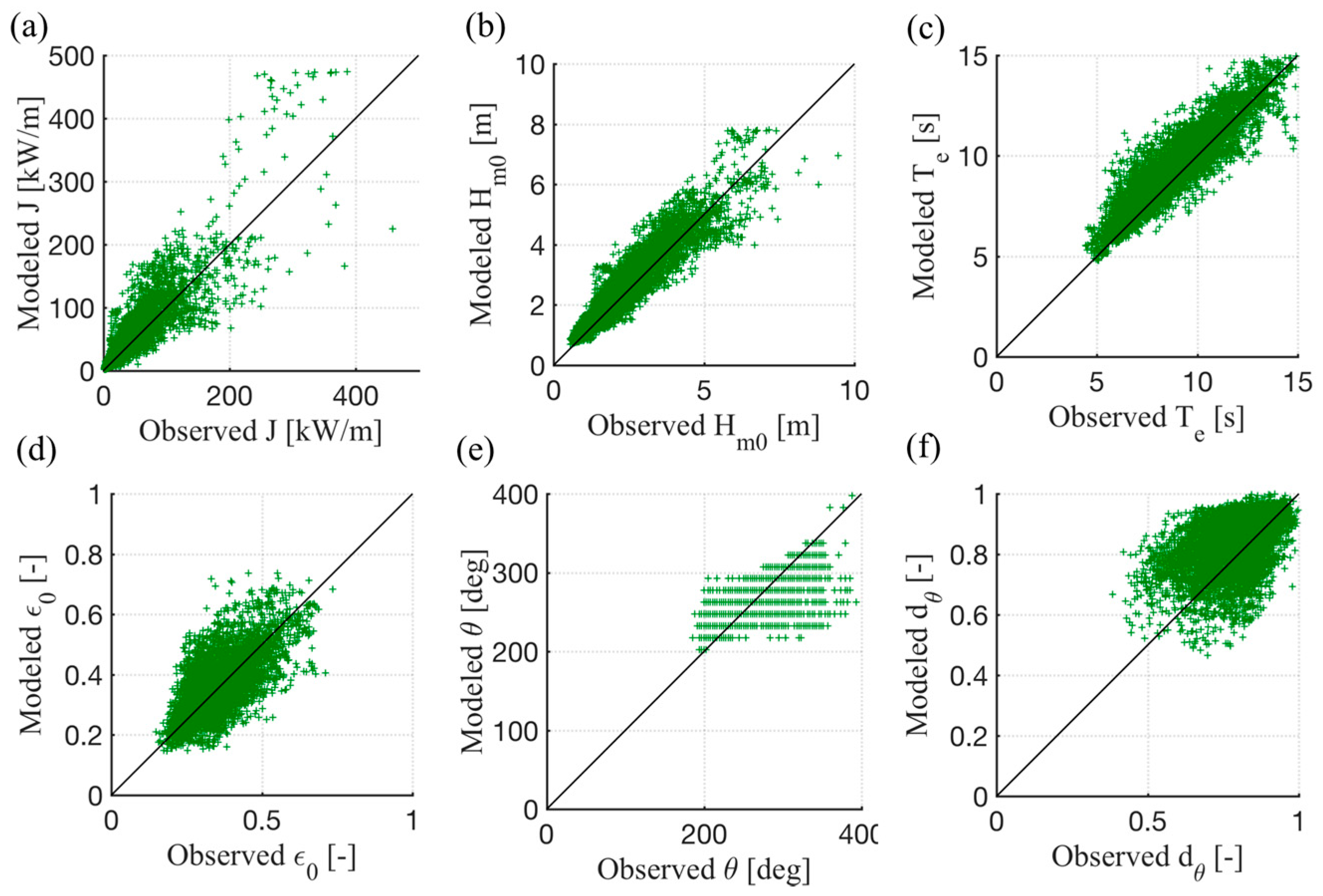
3.2. Model Performance Metrics

The six IEC TS wave resource parameters were calculated from both UnSWAN model results and measured data at NDBC Buoy 46050. Figure 3 shows the comparisons of three representative wave resource parameters―omnidirectional wave power, J_omni; significant wave height, H_m0; and energy period, T_e―between UnSWAN model results forced by WWIII-ST2 simulation and the measurements in 2009. Overall, model predictions for these three wave resource parameters match the observed data well and closely capture the seasonal variations in the measured data. Wave power density and significant wave height are much smaller from June to September than those from November to April, corresponding to the seasonal wind variations in the region.

Model performance was also examined using XY scatter plots for all six wave resource parameters in Figure 4. The XY scatter plots show good correlations between simulated and observed omnidirectional wave power, significant wave height, and energy period, similar to the time-series comparisons in Figure 3. Furthermore, simulated omnidirectional wave power and significant wave height exhibit more scattering for large waves (Figure 4a,b), indicating that the model’s function of predicting large waves under extreme events is less accurate than that under the normal sea-state conditions. In addition, the simulated wave energy periods tend to be slightly larger compared to observed data (Figure 4c). Furthermore, the simulated spectral width falls within the range of 0.2 to 0.7; the small value corresponds to a narrow spectral spread in winter, whereas the large value corresponds to a broad spread in summer [22] (Figure 4d). However, correlations for the direction of the maximum directionally resolved wave power and directionality coefficient are not very strong, as shown in Figure 4e,f.

For each of six wave resource parameters recommended by the IEC TS, the following model performance metrics were computed to show the model skills, which are commonly used in other modeling studies [24,26]. All of these metrics represent an average estimate of the difference between predicted and measured values over a defined period of simulation. The root-mean-square-error (RMSE) is defined as

$$\mathrm{RMSE}=\sqrt{\frac{{{\displaystyle \sum }}_{i=1}^N{\left(X_i-Y_i\right)}^2}{N}}$$

(8)

where $N$ is the number of observed data, $X_i$ is model predictions, and $Y_i$ is the observed data.

RMSE represents the sample standard deviation of the differences between modeled data and measured data.

The percentage error (PE) is defined as

$$\mathrm{PE}(\%)=\frac{100}{N}{{\displaystyle \sum }}_{i=1}^N\left(\frac{X_i-Y_i}{Y_i}\right)$$

(9)

The scatter index (SI) is the RMSE normalized by the average of all measured data $\overline{Y}$

$$\mathrm{SI}=\frac{\mathrm{RMSE}}{\overline{Y}}.$$

(10)

Model bias and percentage bias represent the average difference between the predicted and measured data, which are defined as

$$\mathrm{Bias}=\frac{1}{N}{{\displaystyle \sum }}_{i=1}^N\left(X_i-Y_i\right).$$

(11)

and

$$\mathrm{Bias}(\%)=\frac{{{\displaystyle \sum }}_{i=1}^N{X}_i-{{\displaystyle \sum }}_{i=1}^N{Y}_i}{{{\displaystyle \sum }}_{i=1}^N{Y}_i}·100$$

(12)

The linear correlation coefficient (R) is defined as

$$R=\frac{{{\displaystyle \sum }}_{i=1}^N\left(X_i-\overline{X}\right)\left(Y_i-\overline{Y}\right)}{\sqrt{\left({{\displaystyle \sum }}_{i=1}^N{\left(X_i-\overline{X}\right)}^2\right)\left({{\displaystyle \sum }}_{i=1}^N{\left(Y_i-\overline{Y}\right)}^2\right)}}$$

(13)

The model performance metrics for WWIII simulation (independent runs with ST2 and ST4 packages) and UnSWAN simulation (runs with WWIII boundary conditions when ST2 and ST4 physics were applied respectively) for the six IEC TS parameters are listed in

Table 2. Performance metrics for WWIII and UnSWAN using the ST2 and ST4 physics packages.

Parameter	Model	RMSE	PE (%)	SI	Bias	Bias (%)	R
J (kW/m)	WWIII–ST2	20	32	0.66	6.1	19.7	0.91
	WWIII–ST4	15	25	0.48	2.0	6.5	0.93
	UnSWAN–ST2	21	38	0.68	6.7	21.5	0.90
	UnSWAN–ST4	15	28	0.47	2.9	9.4	0.93
Hs (m)	WWIII–ST2	0.43	9	0.19	0.17	7.3	0.94
	WWIII–ST4	0.36	4	0.16	0.01	0.4	0.95
	UnSWAN–ST2	0.46	12	0.20	0.19	8.5	0.93
	UnSWAN–ST4	0.35	6	0.16	0.05	2.3	0.95
Te (s)	WWIII–ST2	0.99	7	0.11	0.50	5.6	0.90
	WWIII–ST4	1.21	11	0.14	0.86	9.7	0.90
	UnSWAN–ST2	0.94	6	0.11	0.50	5.6	0.91
	UnSWAN–ST4	1.09	9	0.12	0.77	8.6	0.92
${ϵ}_0$	WWIII–ST2	0.07	3	0.20	0.01	1.6	0.67
	WWIII–ST4	0.07	4	0.21	0.01	2.5	0.65
	UnSWAN–ST2	0.07	2	0.20	0.00	1.1	0.71
	UnSWAN–ST4	0.07	6	0.20	0.02	4.7	0.70
$\theta$	WWIII–ST2	22.87	−2	0.08	−6.86	−2.4	0.74
	WWIII–ST4	23.33	−2	0.08	−7.62	−2.7	0.73
	UnSWAN–ST2	22.04	−2	0.08	−6.44	−2.3	0.76
	UnSWAN–ST4	22.17	−2	0.08	−7.26	−2.5	0.76
$d_{\theta }$ (-)	WWIII–ST2	0.10	7	0.13	0.05	6.2	0.48
	WWIII–ST4	0.10	7	0.13	0.05	5.8	0.44
	UnSWAN–ST2	0.10	7	0.13	0.05	5.6	0.51
	UnSWAN–ST4	0.10	6	0.12	0.04	5.4	0.49

. The error statistics for all four model runs are very similar to those in the previous studies conducted in the same region. This indicates that all model runs perform very well and that the results are in good agreement with the observed data at NDBC Buoy 46050. The RMSEs for J_omni, H_s, and T_e are approximately 20 and 21 (kW/m), 0.43 and 0.46 m, 0.99 and 0.94 s, respectively, for WWIII and UnSWAN with the ST2 package. In comparison, the RMSEs for J_omni, H_s, and T_e are about 15 and 15 (kW/m), 0.36 and 0.35 m, 1.21 and 1.09 s, respectively, for WWIII and UnSWAN with the ST4 package. This suggests that WWIII and UnSWAN with the ST4 physics package perform better in simulating J_omni and H_s, but slightly worse in simulating the wave energy period T_e (Table 2). Overall, UnSWAN results have better linear correlation coefficients than WWIII for all six IEC wave resource parameters. Also, for both models, spectral width (${ϵ}_0$), direction of maximum directionally resolved wave power (θ), and the directionality coefficient ($d_{\theta }$), show generally low correlation coefficients. The low correlation coefficient of ${ϵ}_0$ is caused by the higher-order moments of the variance spectrum. For θ and $d_{\theta }$, the low correlation coefficients are due to the uncertainties in both modeled and measured directional metrics [20,22,24].

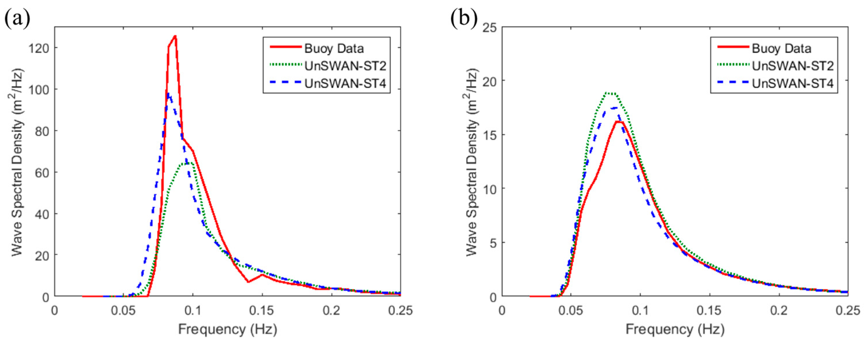
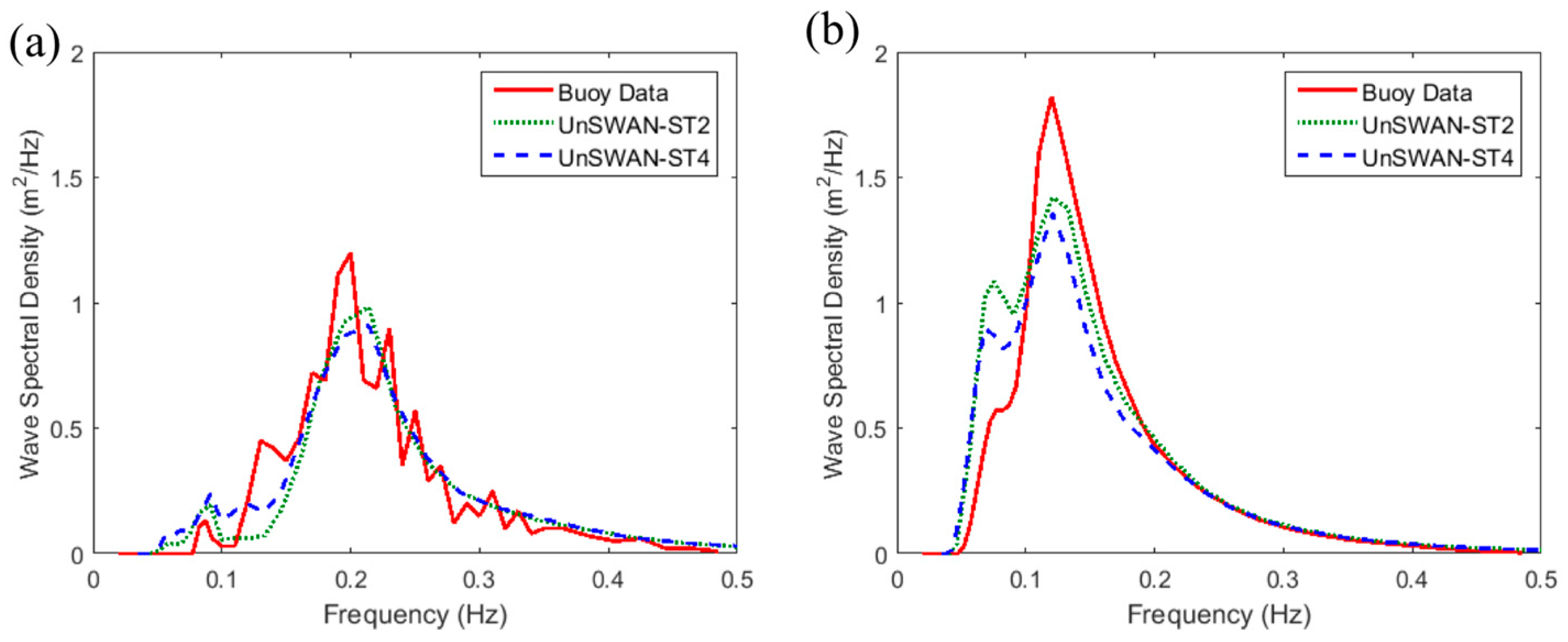
3.3. Evaluation of Physics Packages

To compare the model skills of the ST2 (UnSWAN-ST2) and ST4 (UnSWAN-ST4) physics packages, wave spectra are presented here in terms of radian frequency (ϖ) in Hz and variance density (S) in m²s/rad. Figure 5a compares the predicted and measured wave spectrum at NDBC Buoy 46050 at 5 a.m. on 17 November 2009, the time at which large waves occurred in November. The buoy data show a single swell peak at 0.0875 Hz, and the UnSWAN-ST4 result compares better with the data than the UnSWAN-ST2 result. Figure 5b shows the monthly averaged wave spectrum in November 2009, which confirms that the ST4 package performs better than the ST2 package, as relative to matching the buoy data. The ST4 physics package can improve the model’s ability to predict the significant wave height and timing of large waves because of the better ST4 representation of peak frequency, as shown in Figure 5b. This is consistent with the performance metrics for simulated omnidirectional power in Table 2; the UnSWAN-ST4 result has a smaller over-predicted bias (9.4%) than the UnSWAN-ST2 result (21.5%).

In addition, the modeled and measured wave spectra at NDBC Buoy 46050 at 1 a.m. on 15 July 2009 and the July monthly average are shown in Figure 6a,b, respectively. Model results from UnSWAN-ST2 and UnSWAN-ST4 show a trend similar to the measured data, but slight under-prediction for the spectrum peak (Figure 6b). Figure 6b shows that the swell components (the first peak) are over-predicted while the wind sea components (the second peak) are under-predicted by both ST2 and ST4 physics packages. The ST4 physics package also appears to perform better in simulating swell growth and dissipation.

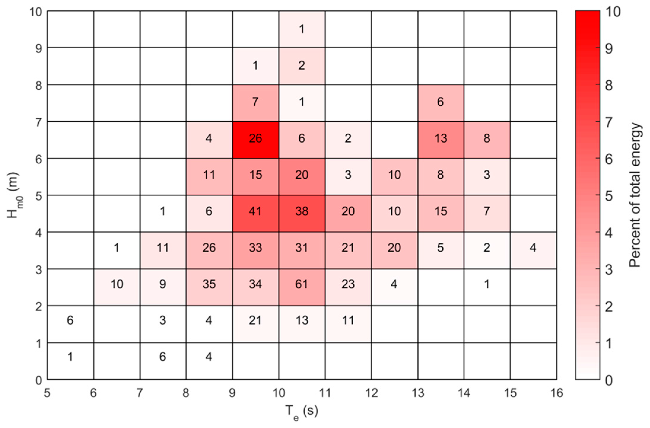
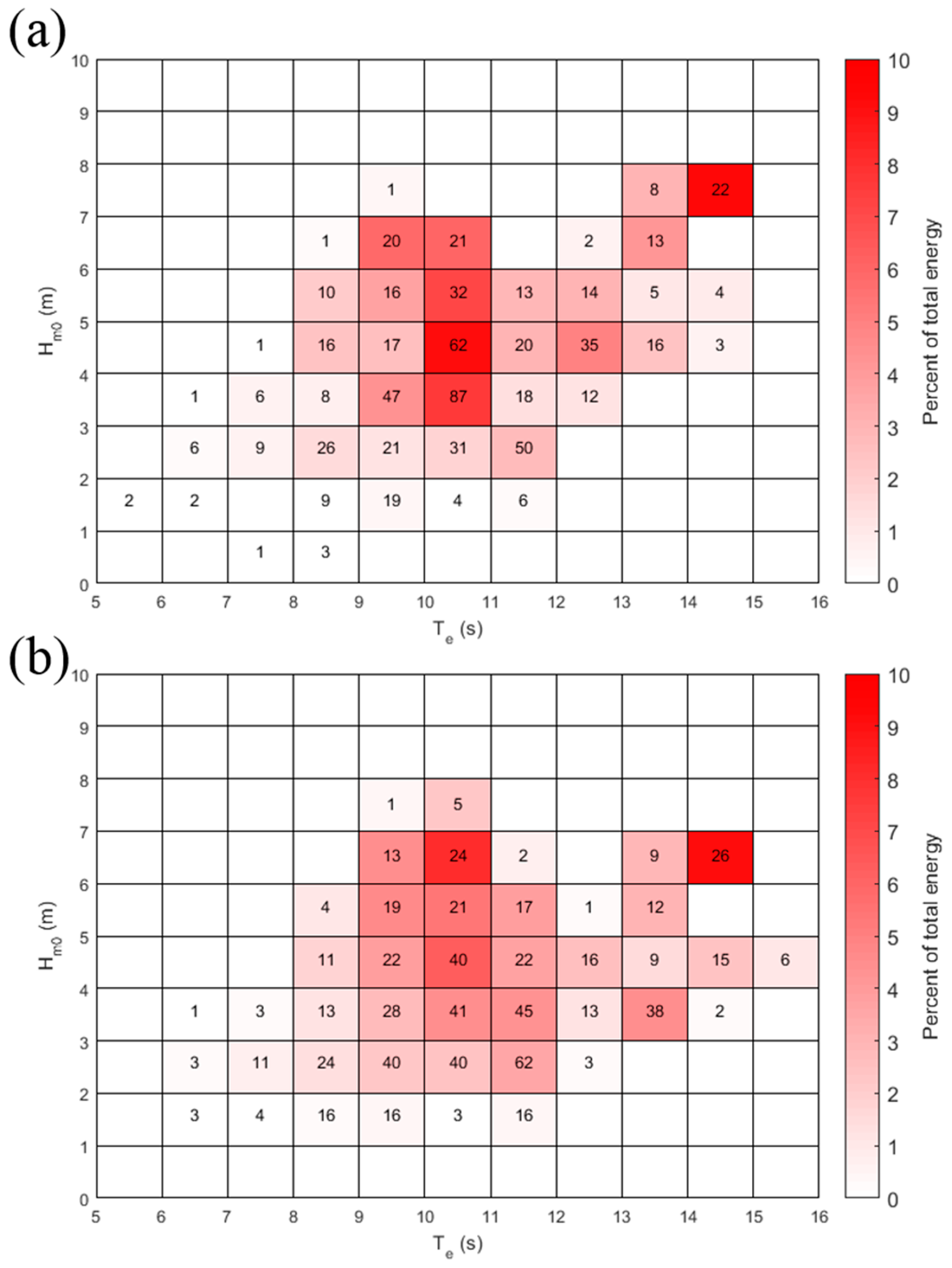
3.4. Bivariate Distributions

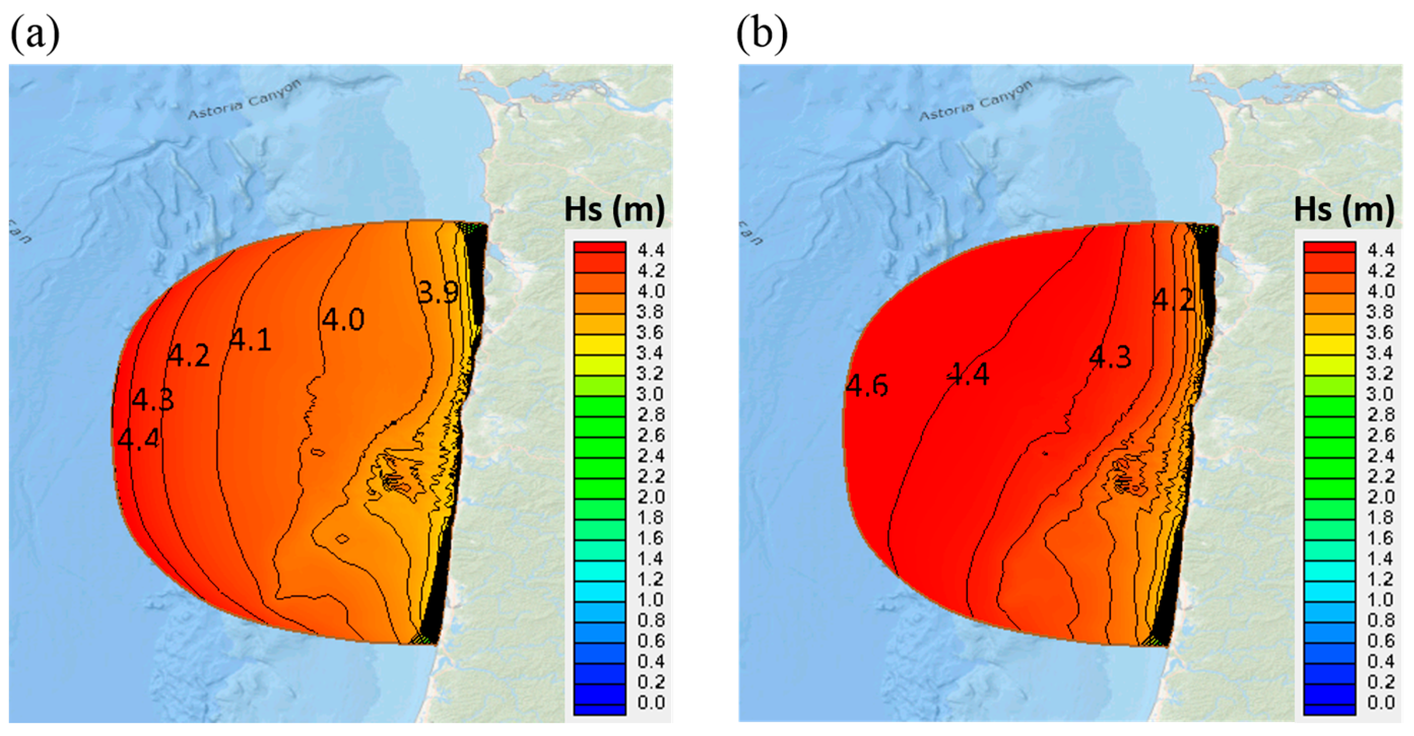
Bivariate distributions are often used to convey the occurrence frequency of the wave climate characteristic defined by significant wave height and energy period [22], and to show the details of the mean annual frequency and energy transport characteristics of wave height and energy period combination [20]. Figure 7 shows the number of hours and the proportion of annual incident energy transport characteristics expected from sea states featuring significant wave height and energy period for buoy observations in the year 2009. Significant wave height is divided into 1 m bins over a range of 0–10 m, and the wave energy period is discretized by 1 s bins over the range of 5–16 s. The frequency in number of hours per year is illustrated by each discrete combination of significant wave height and frequency bins, while the percent of total energy is indicated by the contour color ramp. The maximum-occurring wave state is at H_m0 = (2–3) m and T_e = (11–12) s with occurrence number 61 (Figure 7). The sea states with the maximum significant wave height do not correspond to the percent of total energy, because they only occur at limited times [31]. In comparison, the maximum occurring wave state predicted by UnSWAN-ST2 is 87, which occurred at H_m0 = (3–4) m and T_e = (11–12) s (Figure 8a), while the maximum occurrence number predicted by UnSWAN-ST4 is 62, at H_m0 = (2–3) m and T_e = (11–12) s (Figure 8b). Therefore, UnSWAN-ST4 has an overall better performance than UnSWAN-ST2 in predicting the bivariate distribution of sea state. However, UnSWAN-ST4 predicted the maximum occurrence sea state at the same significant wave height as the measurements, while UnSWAN-ST2 predicted it for the same energy period. This explains why UnSWAN-ST4 has a better modeling ability to predict significant wave height [34], while UnSWAN-ST2 performs slightly better in simulating energy period.

The maximum occurring sea state does not correspond to the sea state with the highest percentage of total energy, because of the contribution from waves with lower significant wave height and energy periods, as shown in Figure 7 and Figure 8. These findings are consistent with Lenee-Bluhm et al. [22]. Red shading is used to differentiate the percent of total energy; dark red color means the greatest contribution to energy. In Figure 7, the maximum percentage of total energy derived from data occurs at H_m0 = (6–7) m and T_e = (9–10) s. On the other hand, the maximum percentage of total energy simulated by UnSWAN-ST2 occurs at H_m0 = (4–5) m and T_e = (10–11) s, and at H_m0 = (7–8) m and T_e = (14–15) s (Figure 8a), while the maximum simulated by UnSWAN-ST4 occurs at H_m0 = (6–7) m and T_e = (11–5) s, and at H_m0 = (6–7) and T_e = (14–15) (Figure 8b). This is indicative of the ST4 physics package being more skilled at simulating significant wave heights and bivariate distributions of maximum energy.

3.5. Wind Effects

Surface wind forcing plays an important role in the accuracy of the wave model hindcast, particularly under extreme wave conditions. To demonstrate the wind effects, a model simulation with UnSWAN in a much larger domain was also conducted. Model performance metrics for simulating the six wave resource parameters using UnSWAN with both the small and larger domains were compared. The UnSWAN (L) has performance metrics (

Table 3. Performance matrix for UnSWAN (L), considering wind effects using the ST4 physics package.

Parameter	UnSWAN (L)–ST4	RMSE	PE (%)	SI	Bias	Bias (%)	R
J (kW/m)	wind	20	39	0.63	6.0	19.2	0.91
	no wind	22	30	0.71	3.7	11.7	0.86
Hs (m)	wind	0.44	12	0.19	0.18	7.8	0.94
	no wind	0.54	5	0.24	0.03	1.3	0.88
Te (s)	wind	0.98	7	0.11	0.56	6.2	0.91
	no wind	1.50	14	0.17	1.05	11.8	0.84
${ϵ}_0$	wind	0.06	2	0.19	0.00	0.7	0.72
	no wind	0.09	−10	0.25	−0.04	−12.2	0.57
$\theta$	wind	21.83	−2	0.08	−7.28	−2.6	0.77
	no wind	26.75	−2	0.09	−8.20	−2.9	0.62
$d_{\theta }$ (-)	wind	0.10	6	0.12	0.04	5.1	0.51
	no wind	0.11	9	0.14	0.06	7.7	0.42

) that are similar to those of UnSWAN in the model domain (UnSWAN–ST4, Table 2). Note that for the six IEC parameters, UnSWAN–ST4 results without wind forcing simulation were similar to UnSWAN–ST4 results with wind simulation, as listed in Table 2. This suggests that for the small domain, the wind effect has no significant impact on the accuracy of the numerical wave hindcast. This finding is consistent with [35].

However, UnSWAN (L)–no wind has a significantly different result than UnSWAN (L) in Table 3. As calculated by Akpinar et al. [32], with a fetch of over 100 km and at a 10 m/s wind speed, a 1.63 m wave height can be fully developed. This is consistent with our model results. Therefore, for a model domain at a scale of 100 km or greater, it is important to consider the wind effect. Figure 9 shows the comparison of monthly averaged significant wave height distributions for no wind and with wind UnSWAN (L) simulations in November 2009. As one can see in Figure 9a, if the wave model does not consider wind effects, the spatial distribution of the significant wave height corresponds to the bathymetry contour shown in Figure 2b, indicating that wave model results are sensitive to bathymetry [34]. The wind forcing significantly changes the wave height spatial distribution (Figure 9b). Similarly, if UnSWAN (L) does not consider the wind effects in summer, when wind speed is generally weaker, the UnSWAN (L)–no wind run also underestimates the significant wave height, as shown in Figure 10 and Table 3. Akpinar et al. [32] showed that low wind speed would underestimate significate wave heights, which also indicates that wind effects play an important role in wave modeling.

4. Conclusions

This paper presents the results of using the unstructured grid SWAN model to simulate the six IEC wave resource parameters at a model domain off the central Oregon coast. The results demonstrate the advantages of unstructured grid wave models in terms of their computational efficiency and grid flexibility for wave resource characterization. The model performance was evaluated using standard performance metrics based on a comparison of the simulations of six wave resource parameters, derived by model hindcasts to those derived from measured data. UnSWAN results show a good agreement with buoy measurements for omnidirectional wave power, significant wave height, and wave energy period. In addition, with better representations of wave growth and dissipation in the WWIII ST4 physics package to provide more accurate open boundary conditions, the UnSWAN model performs generally better than the WWIII model.

Notably, spectral analysis shows that use of the ST4 physics package improves the model’s ability to predict wave spectral density for large waves. Also, a comparison of simulated and measured bivariate distributions of the maximum occurrence of sea state indicated that the ST4 physics package performed better than the ST2 physics package [34], although ST4 and ST2 showed an increased ability to predict significant wave height and wave energy period, respectively.

The sensitivity analysis of wind effect also showed that UnSWAN (L)–no wind has significantly worse results than UnSWAN (L) with wind, indicating that wave modeling with a domain at a scale of O (100 km) or greater needs to consider wind effects. Additional research is needed to investigate wind effects in wave modeling, especially under extreme wave conditions. In summary, this study demonstrated that unstructured grid wave modeling with the ST4 physics package provides advantages for assessing the temporal and spatial variability of wave climates, using high grid resolution near complex geometries, especially within a large model domain.

References

1. Tolman, H.L.; WAVEWATCH III Development Group. User Manual and System Documentation of Wavewatch III® Version 4.18; National Oceanic and Atmospheric Administration, National Weather Service, National Centers for Environmental Prediction: College Park, MD, USA, 2014; 311p.
2. WAMDI Group. The WAM model—A third generation ocean wave prediction model. J. Phys. Oceanogr. 1988, 18, 1775–1810. [Google Scholar]
3. SWAN. SWAN: User Manual, Cycle III Version 41.01AB; Delft University of Technology: Delft, The Netherlands, 2015. [Google Scholar]
4. Benoit, M.; Marcos, F.; Becq, F. TOMAWAC: A prediction model for offshore and nearshore storm waves. In Environmental and Coastal Hydraulics: Protecting the Aquatic Habitat; Proceedings of the Theme B, Volumes 1 & 2; American Society of Civil Engineers: New York, NY, USA, 1997; Volume 27, pp. 1316–1321. ISBN 0-7844-0272-8. [Google Scholar]
5. DHI Mike 21 Spectral Waves FM e Short Description; DHI: Horsholm, Denmark, 2012; Volume 16.
6. Tolman, H.L. Treatment of unresolved islands and ice in wind wave models. Ocean Model. 2003, 5, 219–231. [Google Scholar] [CrossRef]
7. Tolman, H.L. A new global wave forecast system at NCEP. Ocean Wave Meas. Anal. 1997, 2, 777–786. [Google Scholar]
8. EPRI. Mapping and Assessment of the United States Ocean Wave Energy Resource; Electric Power Research Institute: Palo Alto, CA, USA, 2011. [Google Scholar]
9. Yang, Z.; Copping, A. (Eds.) Marine Renewable Energy—Resource Characterization and Physical Effects; Springer International Publishing: Cham, Switzerland, 2017; pp. 37–70. ISBN 978-3-319-53534-0. [Google Scholar]
10. Zijlema, M. Computation of wind-wave spectra in coastal waters with SWAN on unstructured grids. Coast. Eng. 2010, 57, 267–277. [Google Scholar] [CrossRef]
11. Gagnaire-Renou, E.; Benoit, M.; Forget, P. Ocean wave spectrum properties as derived from quasi-exact computations of nonlinear wave-wave interactions. J. Geophys. Res. Ocean. 2010, 115. [Google Scholar] [CrossRef]
12. Cobell, Z.; Zhao, H.; Roberts, H.J.; Clark, F.R.; Zou, S. Surge and Wave Modeling for Louisiana 2012 Coastal Master Plan. J. Coast. Res. 2013, 67, 88–108. [Google Scholar] [CrossRef]
13. Robertson, B.; Bailey, H.; Clancy, D.; Ortiz, J.; Buckham, B. Influence of wave resource assessment methodology on wave energy production estimates. Renew. Energy 2016, 86, 1145–1160. [Google Scholar] [CrossRef]
14. Yuk, J.H.; Kim, K.O.; Jung, K.T.; Choi, B.H. Swell Prediction for the Korean Coast. J. Coast. Res. 2015, 317, 705–712. [Google Scholar] [CrossRef]
15. Sørensen, O.R.; Kofoed-Hansen, H.; Rugbjerg, M.; Sørensen, L.S. A third-generation spectral wave model using an unstructured finite volume technique. In Proceedings of the 29th International Conference on Coastal Engineering, Lisbon, Portugal, 19–24 September 2004; pp. 894–906. [Google Scholar] [CrossRef]
16. Dodet, G.; Bertin, X.; Bruneau, N.; Fortunato, A.B.; Nahon, A.; Roland, A. Wave-current interactions in a wave-dominated tidal inlet. J. Geophys. Res. Ocean. 2013, 118, 1587–1605. [Google Scholar] [CrossRef]
17. Roland, A.; Cucco, A.; Ferrarin, C.; Hsu, T.W.; Liau, J.M.; Ou, S.H.; Umgiesser, G.; Zanke, U. On the development and verification of a 2-D coupled wave-current model on unstructured meshes. J. Mar. Syst. 2009, 78, S244–S254. [Google Scholar] [CrossRef]
18. Roland, A.; Zhang, Y.J.; Wang, H.V.; Meng, Y.; Teng, Y.C.; Maderich, V.; Brovchenko, I.; Dutour-Sikiric, M.; Zanke, U. A fully coupled 3D wave-current interaction model on unstructured grids. J. Geophys. Res. Ocean. 2012, 117. [Google Scholar] [CrossRef]
19. Gallagher, S.; Tiron, R.; Whelan, E.; Gleeson, E.; Dias, F.; McGrath, R. The nearshore wind and wave energy potential of Ireland: A high resolution assessment of availability and accessibility. Renew. Energy 2016, 88, 494–516. [Google Scholar] [CrossRef]
20. Robertson, B.R.D.; Hiles, C.E.; Buckham, B.J. Characterizing the near shore wave energy resource on the west coast of Vancouver Island, Canada. Renew. Energy 2014, 71, 665–678. [Google Scholar] [CrossRef]
21. IEC (International Electrotechnical Commission). Marine Energy—Wave, Tidal and Other Water Current Converters—Part 101: Wave Energy Resource Assessment and Characterization; IEC TS 62600-101; Edition 1.0.2015-06; International Electrotechnical Commission: Geneva, Switzerland, 2015. [Google Scholar]
22. Lenee-bluhm, P.; Paasch, R.; Özkan-haller, H.T. Characterizing the wave energy resource of the US Pacific Northwest. Renew. Energy 2011, 36, 2106–2119. [Google Scholar] [CrossRef]
23. Akpinar, A.; Kömürcü, M.I. Assessment of wave energy resource of the Black Sea based on 15-year numerical hindcast data. Appl. Energy 2013, 101, 502–512. [Google Scholar] [CrossRef]
24. García-Medina, G.; Özkan-Haller, H.T.; Ruggiero, P. Wave resource assessment in Oregon and southwest Washington, USA. Renew. Energy 2014, 64, 203–214. [Google Scholar] [CrossRef]
25. García-Medina, G.; Özkan-Haller, H.T.; Ruggiero, P.; Oskamp, J. An Inner-Shelf Wave Forecasting System for the U.S. Pacific Northwest. Weather Forecast. 2013, 28, 681–703. [Google Scholar] [CrossRef]
26. Yang, Z.; Neary, V.S.; Wang, T.; Gunawan, B.; Dallman, A.R.; Wu, W. A wave model test bed study for wave energy resource characterization. Renew. Energy 2017, 1–13. [Google Scholar] [CrossRef]
27. Soares, C.G.; Bento, A.R.; Gonçalves, M.; Silva, D.; Martinho, P. Numerical evaluation of the wave energy resource along the Atlantic European coast. Comput. Geosci. 2014, 71, 37–49. [Google Scholar] [CrossRef]
28. Gonçalves, M.; Martinho, P.; Guedes Soares, C. Wave energy conditions in the western French coast. Renew. Energy 2014, 62, 155–163. [Google Scholar] [CrossRef]
29. Silva, D.; Bento, A.R.; Martinho, P.; Guedes Soares, C. High resolution local wave energy modelling in the Iberian Peninsula. Energy 2015, 91, 1099–1112. [Google Scholar] [CrossRef]
30. Bento, A.R.; Martinho, P.; Guedes Soares, C. Numerical modelling of the wave energy in Galway Bay. Renew. Energy 2015, 78, 457–466. [Google Scholar] [CrossRef]
31. Morim, J.; Cartwright, N.; Etemad-Shahidi, A.; Strauss, D.; Hemer, M. Wave energy resource assessment along the Southeast coast of Australia on the basis of a 31-year hindcast. Appl. Energy 2016, 184, 276–297. [Google Scholar] [CrossRef]
32. Akpinar, A.; van Vledder, G.P.; Kömürcü, M.I.; Özger, M. Evaluation of the numerical wave model (SWAN) for wave simulation in the Black Sea. Cont. Shelf Res. 2012, 50–51, 80–99. [Google Scholar] [CrossRef]
33. Moeini, M.H.; Etemad-Shahidi, A.; Chegini, V.; Rahmani, I. Wave data assimilation using a hybrid approach in the Persian Gulf. Ocean Dyn. 2012, 62, 785–797. [Google Scholar] [CrossRef]
34. Amrutha, M.M.; Kumar, V.S.; Sandhya, K.G.; Nair, T.M.B.; Rathod, J.L. Wave hindcast studies using SWAN nested in WAVEWATCH III—Comparison with measured nearshore buoy data off Karwar, eastern Arabian Sea. Ocean Eng. 2016, 119, 114–124. [Google Scholar] [CrossRef]
35. Strauss, D.; Mirferendesk, H.; Tomlinson, R. Comparison of two wave models for Gold Coast, Australia. J. Coast. Res. 2007, 50, 312–316. [Google Scholar]
36. Tolman, H.L.; Chalikov, D. Source Terms in a Third-Generation Wind Wave Model. J. Phys. Oceanogr. 1996, 26, 2497–2518. [Google Scholar] [CrossRef]
37. Ardhuin, F.; Rogers, E.; Babanin, A.V.; Filipot, J.-F.; Magne, R.; Roland, A.; van der Westhuysen, A.; Queffeulou, P.; Lefevre, J.-M.; Aouf, L.; et al. Semiempirical Dissipation Source Functions for Ocean Waves. Part I: Definition, Calibration, and Validation. J. Phys. Oceanogr. 2010, 40, 1917–1941. [Google Scholar] [CrossRef]
Figure 1. The UnSWAN model domain (red box) off the central Oregon coast, along with the location of the National Oceanic and Atmospheric Administration National Data Buoy Center (NDBC) Buoy 46050. The nested WWIII model domains include a global grid (L1, not indicated on the map) and two intermediate grids (L2 and L3).
Energies 11 00605 g001
Figure 2. (a) The UnSWAN (L) model grid and (b) the bathymetric contours.
Energies 11 00605 g002
Figure 3. Hourly time-series comparison of three representative International Electrotechnical Commission (IEC) wave resource parameters between UnSWAN (ST2) predictions and observed data over the one-year period of 2009 at NDBC Buoy 46050. The open-boundary condition of UnSWAN is forced with the model output of WWIII, using the ST2 physics package.
Energies 11 00605 g003
Figure 4. XY scatter plots of six IEC wave resource parameters for UnSWAN, using the ST2 physics package versus observed data. The solid black line indicates the 1:1 line.
Energies 11 00605 g004
Figure 5. Measured and modeled wave spectra at NDBC Buoy 46050 (a) at 5 a.m. on 17 November 2009; and (b) the November monthly average, 2009.
Energies 11 00605 g005
Figure 6. Measured and modeled wave spectra at NDBC Buoy 46050 (a) at 1 a.m. on 15 July 2009; and (b) the July monthly average, 2009.
Energies 11 00605 g006
Figure 7. Bivariate distribution of occurrence and energy showing the probability and energy distribution defined by significant wave height and energy period. The results are calculated from the field data at NDBC 46050 in 2009.
Energies 11 00605 g007
Figure 8. (a) UnSWAN-ST2 and (b) UnSWAN-ST4 bivariate distribution of occurrence and energy showing the probability and energy distribution defined by significant wave height and energy period.
Energies 11 00605 g008
Figure 9. Modeled 2D significant wave height distributions with UnSWAN (L): (a) no wind—November average, 2009; (b) with wind—November average, 2009.
Energies 11 00605 g009
Figure 10. Modeled 2D significant wave height distribution with UnSWAN (L) (a) no wind—July average, 2009; (b) with wind—July average, 2009.
Energies 11 00605 g010