Application of the Mohr-Coulomb Yield Criterion for Rocks with Multiple Joint Sets Using Fast Lagrangian Analysis of Continua 2D (FLAC2D) Software


1
Institut für Geotechnik, Technische Universität Bergakademie Freiberg, Freiberg 09599, Germany
2
School of Mechanics & Civil Engineering, China University of Mining & Technology, Beijing 100083, China
*
Author to whom correspondence should be addressed.
Energies 2018, 11(3), 614; https://doi.org/10.3390/en11030614
Submission received: 6 February 2018
/
Revised: 2 March 2018
/
Accepted: 6 March 2018
/
Published: 9 March 2018
Abstract
:The anisotropic behavior of a rock mass with persistent and planar joint sets is mainly governed by the geometrical and mechanical characteristics of the joints. The aim of the study is to develop a continuum-based approach for simulation of multi jointed geomaterials. Within the continuum methods, the discontinuities are regarded as smeared cracks in an implicit manner and all the joint parameters are incorporated into the equivalent constitutive equations. A new equivalent continuum model, called multi-joint model, is developed for jointed rock masses which may contain up to three arbitrary persistent joint sets. The Mohr-Coulomb yield criterion is used to check failure of the intact rock and the joints. The proposed model has solved the issue of multiple plasticity surfaces involved in this approach combined with multiple failure mechanisms. The multi-joint model was implemented into Fast Lagrangian Analysis of Continua software (FLAC) and is verified against the strength anisotropy behavior of jointed rock. A case study considering a circular excavation under uniform and non-uniform in-situ stresses is used to illustrate the practical application. The multi-joint model is compared with the ubiquitous joint model.
1. Introduction
The behavior of a jointed rock (within this paper this term includes also jointed rock masses) is anisotropic, non-linear and stress path dependent due to the presence of discontinuities. Compared to intact rock, jointed rock generally exhibit reduced stiffness, higher permeability and lower strength. Various analytical, numerical and empirical methods are suggested in order to take into account the influence of discontinuities on the mechanical behavior of jointed rock [1,2,3,4,5,6]. In the past several decades, a lot of lab tests with samples containing a single or multiple joint sets under confined and unconfined conditions have been implemented to investigate the joint orientation effect [7,8,9]. With the ongoing development of computer based simulation techniques, more sophisticated models have been developed in recent years and it is possible to incorporate more aspects into the simulations [10,11,12,13].
Two numerical techniques are common in rock mechanics: continuum-based methods and discontinuum based methods. Discontinuum methods consider the rock mass as an assemblage of rigid or deformable blocks connected along discontinuities [14], and investigate the microscopic mechanisms in granular material and crack development in rocks [3,15]. Boon et al. [16] performed 2D discrete element analyses to identify potential failure mechanisms around a circular unsupported tunnel in a rock mass intersected by three independent joint sets. In continuum methods, the discontinuities are considered as smeared planes of weakness (joints) incorporated in each zone. The equivalent continuum method contains three parts: the equivalent continuum compliance part (incremental elastic law), the yield criterion and the plastic corrections part.
Will [17] implemented a multi-surface plasticity model into a finite element code with internal iterations in case that several plasticity surfaces are touched at the same time. Zhang [18] developed further the Goodman’s joint element model and derived the equivalent method for rock masses with multi-set joints in a global coordinate system. Rihai [19,20] proposed a method which takes into account the influence of micro moments on the behavior of the equivalent continuum based on the Cosserat theory. Hurley et al. [21] presented a numerical method which implemented the method into GEODYN-L code. This method uses a series of stress and strain-rate update algorithms to rule joints closure, slip, and stress distribution inside the computational cells which contain multiple embedded joints. A model with multi-sets of ubiquitous joints with an extended Barton empirical formula was proposed by Wang [22] and pre- and post-peak deformation characteristics of the rock mass were also considered. Many models have been formulated to simulate the effect of joint angle on the strength and deformability of rock masses, but only a few consider several joint sets having different strength parameters and their effects on failure characteristics.
This paper presents a new equivalent continuum constitutive model named multi-joint model to simulate the behavior of jointed rock. This model is suited for jointed rock containing up to three arbitrary joint sets with corresponding spatial distribution. The equivalent compliance matrix of the rock mass is established and the Mohr-Coulomb yield criterion is used to check the failure characteristics of the intact rock and the joints. A circular tunnel subjected to uniform and non-uniform in-situ stresses is used to illustrate the application of this model.
2. Methodology for Equivalent Continuum Multi-Joint Model
2.1. Ubiquitous Joint and Related Approaches
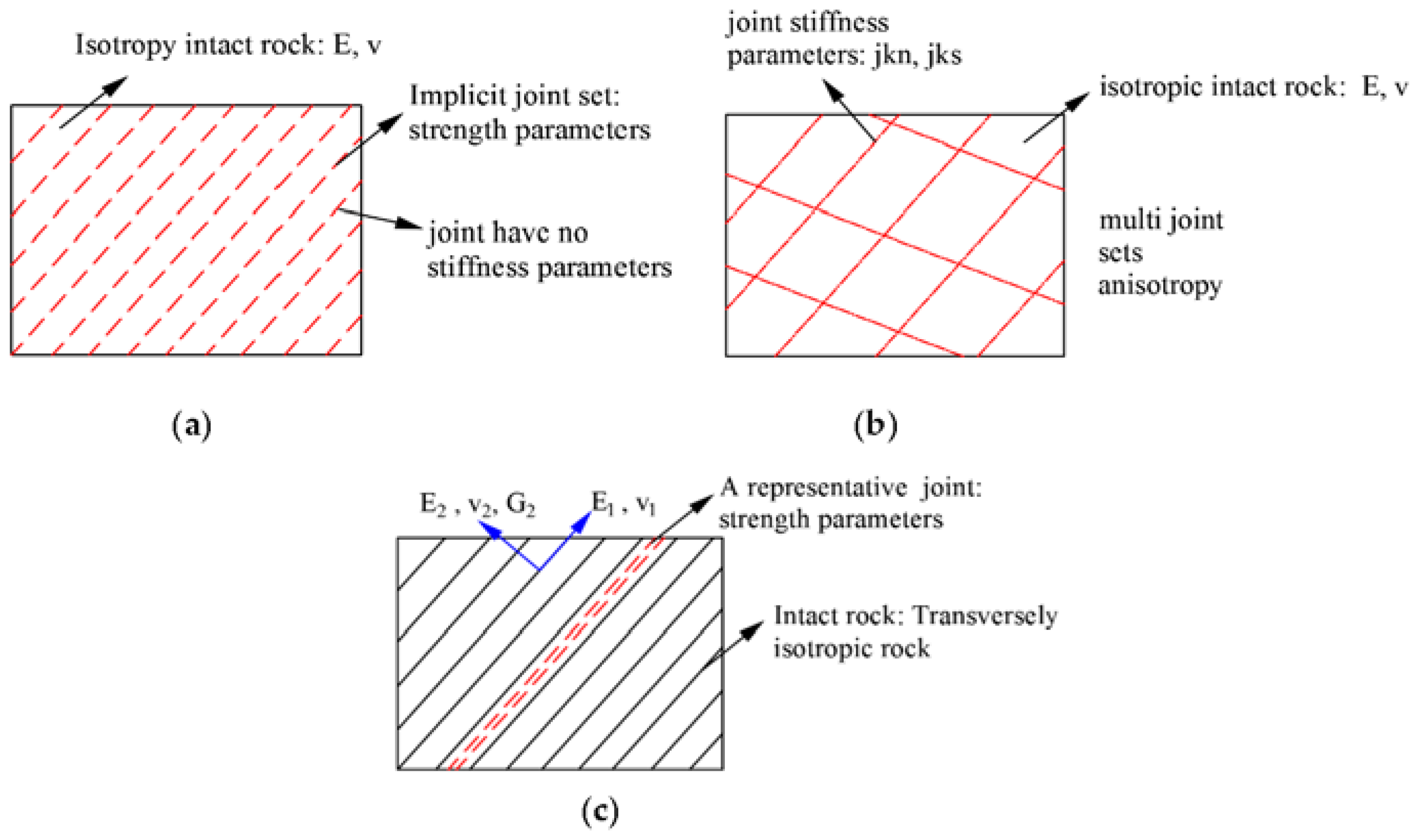
The term ‘ubiquitous joint’ used by Goodman [23] implies that the joint sets may occur at any point in the rock mass without a fixed location. The joints are embedded in a Mohr-Coulomb solid (Figure 1a).
Failure may occur in either the rock matrix or along the joints, or both, according to the stress state, the orientation of the joints and the parameters of matrix and joints [24]. More advanced models based on ubiquitous joint or strain-harding/softening ubiquitous joint (subiquitous) were developed in recent years [13,22,25,26,27] as shown in Figure 1b,c. These approaches consider aspects like stiffness anisotropy in addition to the strength anisotropy, joint spacing, strain softening or bi-linear strength envelopes. The proposed multi-joint model is characterized by different strength parameters and considers overall stiffness reduction due to the joints like shown in Figure 2.
2.2. Elastic Matrix of the Equivalent Continuum Model
The elastic stiffness properties of the joints are denoted by the joint normal and shear stiffness parameters kn and ks, respectively. The spatial characteristics of the joint sets are represented by joint orientation and spacing. The multi-joint model incorporates the joint parameters by an overall downgrading of the rock matrix parameters, so that in terms of stiffness still isotropic behavior is assumed. The corresponding strain-stress relationship is given by the following expression:
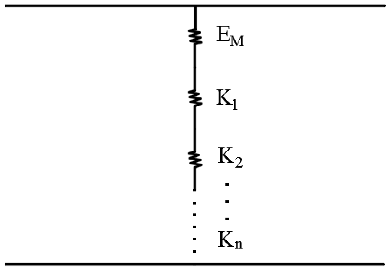
In this matrix, Eeq is the equivalent deformation modulus of the rock mass, G is shear modulus and ν is Poison’s ratio of the intact rock. If n is the number of joint sets, Si is the number of joints per 1 meter for joint set i, Ki is the stiffness of joint set i and EM means Young’s modulus of the intact rock matrix, then the equivalent deformation modulus is obtained:
Consequently, the corresponding Young’s modulus of the rock mass is related to the joint spacing and the joint stiffness. Springs in series representing matrix and joint stiffness will lead to significant reduction in overall stiffness as shown in Figure 3.
2.3. Failure Criterion of Multi-Joint Model
Plasticity leads to irreversible deformations after reaching the yield condition. For the multi-joint model the return mapping procedure is used. Figure 4 elucidates possible geometric conditions arising from the intersection of two yield surfaces (F1 and F2) representing tensile (F1) and shear (F2) failure. Several different situations have to be considered [28]: (1) If only one yield condition is violated (region s4 and s5), plasticity correction is performed by the corresponding potential functions. (2) If more than one yield condition is violated, the situation can be categorized as follows:
- (a)
- If Ftrial (σ,εpl) > 0 and λαi + 1 > 0, for both α = 1 and 2 (region s12) both surfaces are active [19].
- (b)
- If Ftrial (σ,εpl) > 0 and λαi + 1 < 0, for α = 1 or 2 (region s1 or s2) only one of the surfaces are active.
where Ftrial is the failure criterion for the yield surface and λ is the plastic multiplier [29,30].
Jaeger [2] introduced the plane of weakness model which focus on the shear failure of anisotropic rocks. Within the multi-joint model Mohr’s stress circle can be used to interpret the jointed rock strength for different constellations of joint orientation and direction of loading. In case of uniaxial compression with only one single joint set, Mohr’s stress circle representation is shown in Figure 5.
Point A indicates the critical failure stage for a joint. Joint angle αj identifies the corresponding failure plane:
where ϕj is the joint friction angle, αj is the critical joint angle measured from horizontal direction.
fs,0 and ft,0 are the shear and tension failure criteria for the rock matrix. fs,1 and ft,1 are the shear and tension failure criteria of the joint set. The shear strength criterion for this rock mass can be expressed as:
where c and ϕ are cohesion and internal friction angle for the matrix. cj and ϕj are joint cohesion and joint friction angle. With increasing vertical stress, the intersection area between Mohr’s stress circle and joint shear failure envelop grows as illustrated in Figure 6.
The general expressions for the maximum and minimum failure angles are:
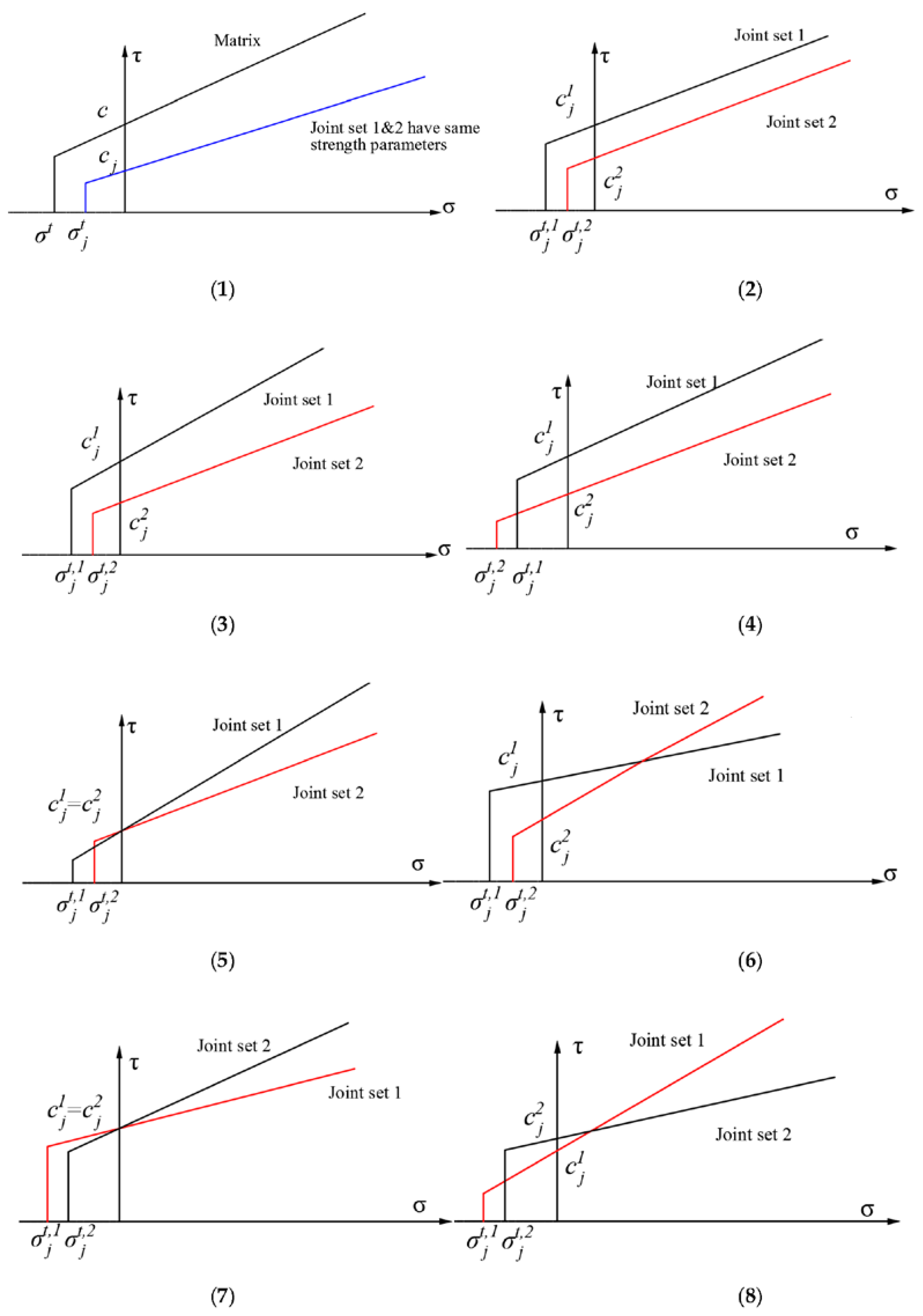
Point A indicates the orientation of the plane with minimum strength. Jaeger’s complete curve, which shows the relationship between the joint angle and uniaxial compressive strength is shown in Figure 7. If a jointed rock has more than one sets of joints, the potential failure modes which have to be considered increase. The different joints can have either identical strength parameters but different joint angles, or they have also different strength parameters. Eight typical joint parameters constellations are shown in Table 1 and in Figure 8.
There are two constellations for a rock mass which has two joints with different strength parameters: (I) one joint is weaker in all strength parameters (series 2–4 in Table 1) and (II) strength parameter have different relations to each other (series 5–8).
In order to determine the failure region of the two joints, several Mohr’s circles and the corresponding schemes are drawn. Exemplarily, Figure 9 illustrates that joint set 1 has lower strength values compared to joint set 2. In Figure 9a, the point A represents the least failure angle for joint set 2. At this stage for joint set 1, there is a region from B to C that fails.
When the stress increases towards the critical state in the rock matrix, the angle of the failure range for each joint is different (Figure 9b). If the jointed rock only has joint set 1, the FOG area in Figure 9c is the joint set failure range. If the rock mass has joint set 2 only, the gray area DOE represents the failure area. As can be seen in Figure 9c, there is a significant difference between the area of DOE and FOG. If both joint sets are in zone BOC, failure may easily occurs on joint 1. Compared with the black and grey regions, the joint set 2 might also reach the critical state when joint set 1 is located in region FOB or COG.
Two types of joint failure criteria for a rock mass are discussed here. For constellations 1–4 in Table 1, a new function h is introduced into the σ-τ-plane in order to solve the multi-surface plasticity problem. This function h is represented by the diagonal between the representation of fs,1 = 0 and ft,1 = 0. According to Figure 10a, the failure areas are divided into four sections. If shear failure is reached on the plane in Sections 1 and 2, the stress point will brought back to the curve fs,1 = 0. If the stress state belongs to the Section 3 or 4, local tensile failure takes place and the stress point will brought back to ft,1 = 0.
For the constellations 5–8 in Table 1, two new functions h1 and h2 were introduced in the τ-σ-plane in order to solve the multi-surface plasticity problem. Function h1 represents the diagonal between fs,1 = 0 and ft = 0. Function h2 represents the diagonal between fs,1 = 0 and fs,2 = 0. The stress state which violates the joint failure criterion will be located in sections 1 to 8 corresponding to positive or negative domain of ft = 0, fs,1 = 0, fs,2 = 0, h1 = 0 and h2 = 0. According to Figure 10c, if for the second joint set shear failure is detected on the plane in sections 1 and 2, the stress will be brought back to the curve fs,2 = 0. If for the first joint set shear failure is detected in sections 3, 4 and 5, the stress will be brought back to the curve fs,1 = 0. If the stress state belongs to section 6, 7 or 8, local tensile failure takes place and the stress will be brought back to ft = 0. ft = 0 is the minimum tension failure criterion for the two joints inside a rock mass.
2.4. Numerical Implementation
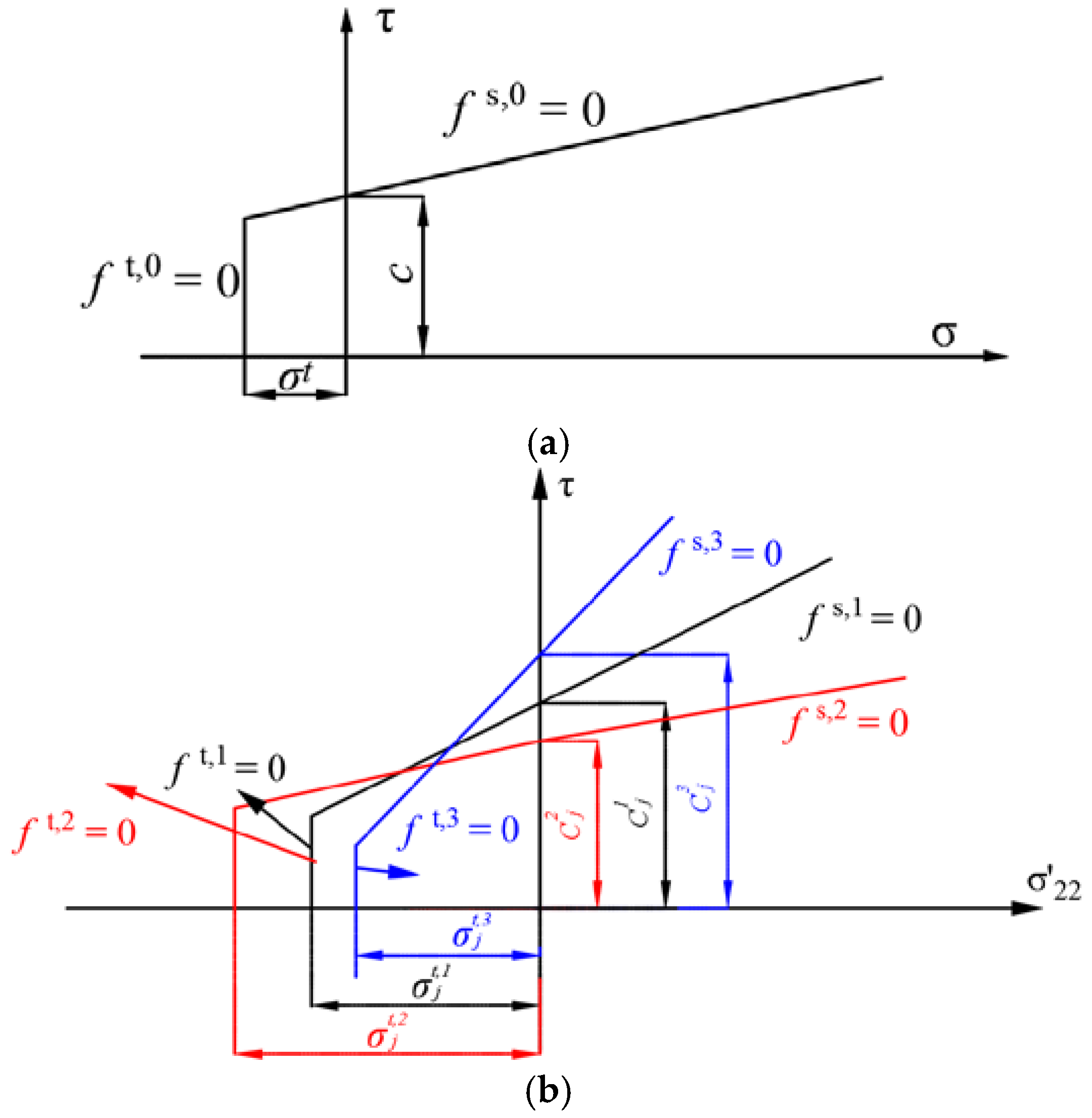
The above-mentioned Mohr-Coulomb yield criteria for the multi-joint model is programmed as a user defined model and implemented into the 2-dimensional explicit finite difference code FLAC [31]. The joints are embedded in a Mohr-Coulomb matrix. The failure criterion of the intact rock (matrix) is represented in the plane (σ, τ) and shown in Figure 11a. Equations (8) and (9) shows the failure envelops and plastic potentials for rock matrix and joints.
The yield criterion for each joint is a Mohr-Coulomb failure criterion with tension cut-off. Flow rule for shear failure is non-associated, and the tension flow rule is associated. For the joint set i (i = 1, 3), the local failure envelops are defined as fs,i and ft,i according to the following equations:
where , and σt,i represent the friction, cohesion and tensile strength for joint set i. If ≠ 0, the tensile strength cannot be larger than σt,imax. = || stand for the magnitude of the tangential stress component of a joint, and the corresponding strain variable is γji. For the multi-joint model, three joint sets have six failure criterions in the (, τ) plane, as illustrated in Figure 11b.
In Figure 11, strength envelops for three joint sets with independent strength parameters are presented. Obviously, various types of failure can occur in each computational step, including single or simultaneous shear yielding on 1, 2 or 3 weak planes, tensile failure on one or more joints as well as combined shear and tensile failure. In each calculation step the failure of the intact rock and the joint sets are checked, the code also checks for multiple active yield surfaces. After each stress increment, general failure through the intact rock is first checked and if there is any violation of the failure criterion, the corresponding plastic stress correction is applied. According to the updated stress state, potential failure of each joint set is checked. The flowchart shown in Figure 12 illustrates the operating principle of this law. A detailed description is provided by Chang [32].
3. Verification of Multi-Joint Model
To validate the proposed multi-joint model, a series of calculation cases including triaxial and uniaxial compressive tests with two perpendicular or three joints were selected and compared with analytical solutions in this section.
3.1. Analytical Solution for a Jointed Rock Sample
The analytical solution for a jointed rock can be expressed using the shear and normal stresses acting on the fracture plane as illustrated in Figure 13. Formulas are given below:
Slip will occur along a joint in a specimen when:
where cj is the joint cohesion, ϕj is the joint friction angle and β is the joint angle formed by vertical stress and the joint. In an uniaxial compressive test, the maximum stress of a jointed rock can be expressed as:
Bray [6] suggested that the overall strength of a rock mass containing multiple joints is given by the lowest strength of the individual strength relations. Final equations defining the uniaxial compressive strength of a rock specimen containing multiple joints can be expressed as:
The uniaxial compressive strength σc calculated by Equation (13) determines the minimum strength of a rock mass for various joint combinations and used for analytical solutions in the following section.
3.2. Strength Anisotropy of a Rock Mass Containing Two Perpendicular Joints
3.2.1. Uniaxial Compressive Tests
The variation of strength for a jointed rock containing two perpendicular joints under uniaxial compression is shown in Figure 14. Mechanical properties of the rock matrix and the joints are listed in Table 2.
Figure 14a illustrates the analytical solution for the strength envelope considering both, the effective and the non-active joint. The colored curves in Figure 14a correspond to the colored joints shown in Figure 14b. In Point A and E the two joints are horizontal and vertical, respectively. Points B and D describe the critical joint position. Point C is the inflection point for the two curves. From position A to E, the two joints with fixed inclination to each other are rotated by 90 degrees.
In this section, two more situations for a sample with two perpendicular joints having different strength parameters are discussed. The two joints can have only different joint friction angles or have various joint cohesion values. Specific parameters are listed in Table 3 and Table 4. The jointed rock strength behavior is shown in Figure 15 and Figure 16.
3.2.2. Triaxial Compressive Tests
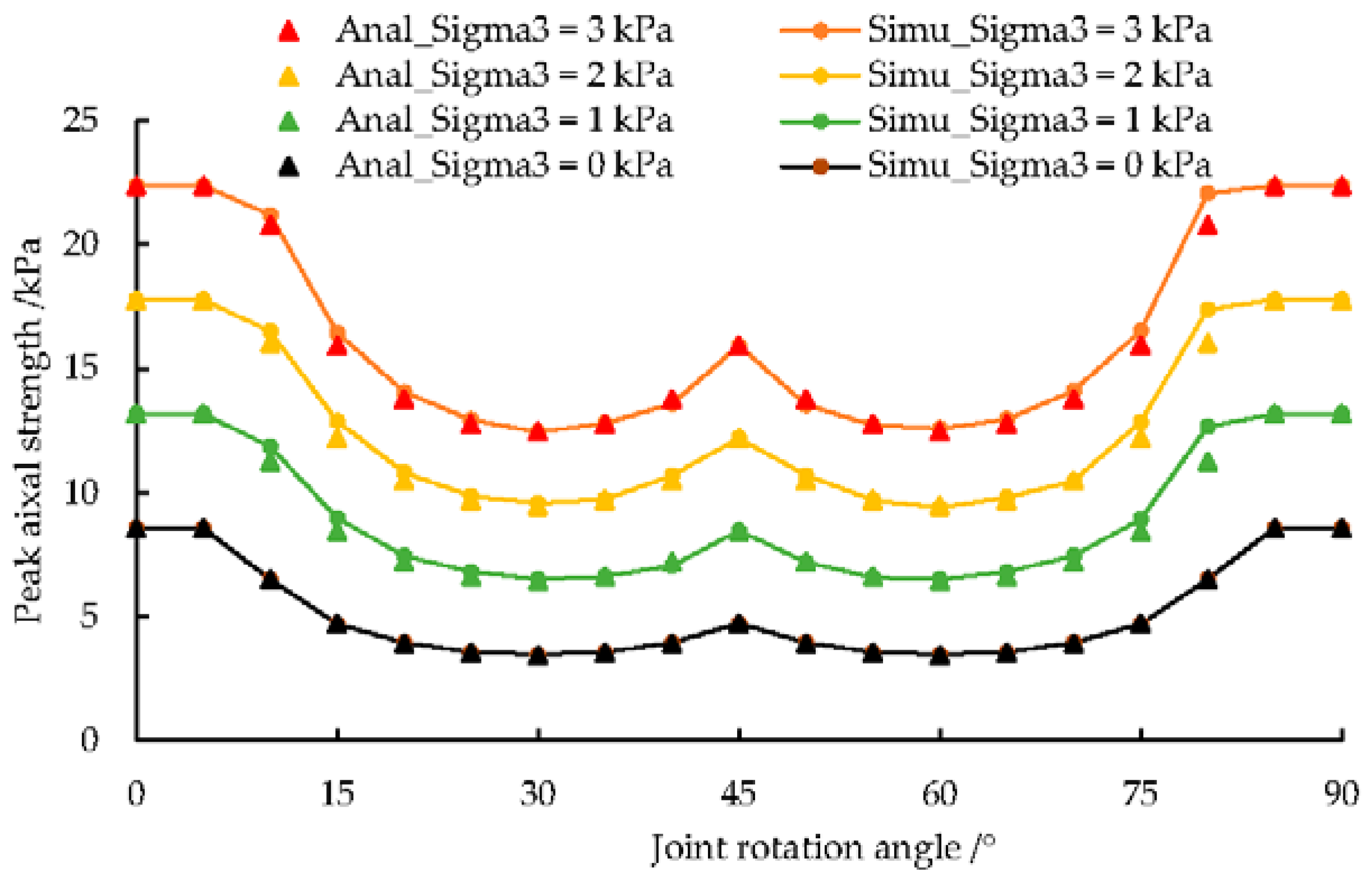
Specimens with different joint orientations are subjected to triaxial compression at various confining pressures. Figure 17 compares the multi-joint model simulation results for samples with two perpendicular joints with corresponding analytical solutions (see Section 3.1). The jointed rock properties are listed in Table 2 (see Figure 17). The match is excellent, with a relative error smaller than 1% for all joint angles. The black curve demonstrates the anisotropic behavior of the model without confining pressure (uniaxial compression test as shown in Section 3.2.1). A strength reduction is observed for joint angles from 5° to 30°. A local strength increase is observed for joint angles at 45° ± 15°.
Finally, the strength increases for joint angles from 60° to 85°. Increasing confining pressure shifts the failure envelope upwards and the curve shape becomes more pronounced. Increasing confining pressures leads to a broader curve shoulder (enlargement from 5° to 15° and from 80° to 90°). The strength anisotropy curve for two perpendicular joints has a W shape and is consistent with experiments of Ghazvinian et al. [9]
3.3. Strength Prediction for Three Joints
Behavior of a sample with three joints under uniaxial compression is documented in Figure 18. The minimum angle between each joint is 30°. Point A, B and D describes the critical joint positions. Point C represents the peak strength value. UCS varies from 3.5 kPa to 4.73 kPa, while the maximum UCS for one or two joints is around 8.5 kPa. Compared with the analytical solution, the modeling results show a good match for all joint angles. The strength anisotropy behavior for rock with one joint is characterized by U or V shape (Jaeger’s curve). The curve for sample with two perpendicular joints has a W form. In case of three joints, three local peak values appear (see Figure 18b).
4. A Case Study: Tunnel Excavation
A circular tunnel subjected to an initial stress state is depicted in Figure 19. The objective of this model is to investigate the mechanical response of a circular excavation under either uniform or non-uniform in-situ stresses. The geometry of the numerical model is characterized by a tunnel with diameter of D = 1.5 m and a quadratic model size of W = 10 m. σyy is set to 1 MPa and the other input parameters are shown in Table 5. Three cases are studied under different in-situ stresses. The vertical earth pressure coefficient κ is set to 1.0, 0.5 and 2.0, respectively (Table 6). A value of κ > 1 means that in-situ horizontal stress is greater than in-situ vertical stress and vice versa. Constellations with no joint, one joint and two joints were investigated. The developed multi-joint model containing two joint sets is compared with the ubiquitous joint model with only one joint set.
4.1. Simulation Results for Ubiquitous Joint Model
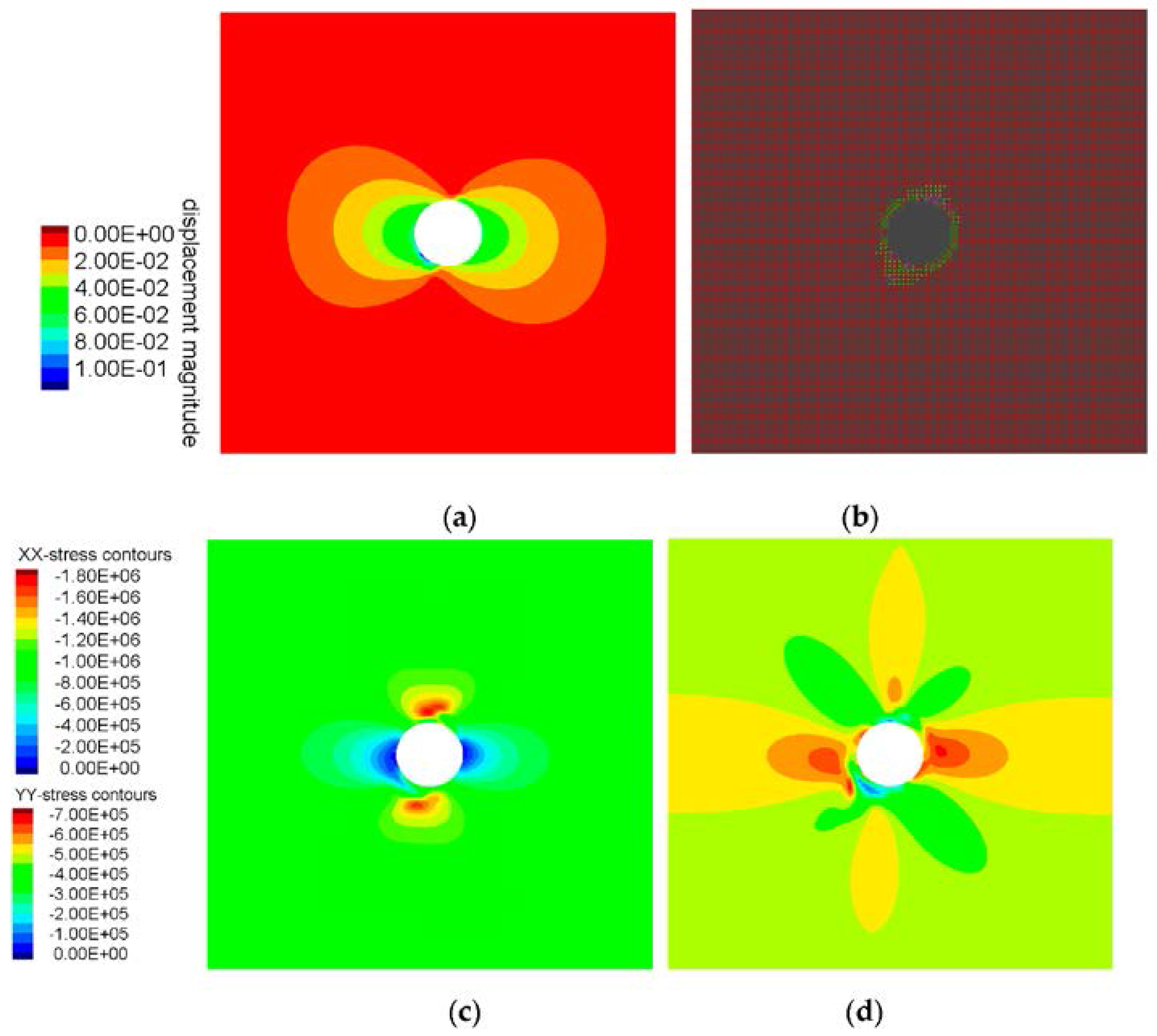
This simulations are based on the standard ubiquitous joint model with joint angle of −60° (measured anticlockwise from vertical direction). Figure 20, Figure 21 and Figure 22 show contour plots of displacement magnitude and stress components as well as the plasticity state for different stress fields.
Figure 20 shows maximum displacements of 0.12 m at the tunnel boundary around 30° inclined to the vertical. Plasticity pattern follows the displacement field. (Figure 20a,b). The influence of the joint on the secondary stress field is illustrated by Figure 20c,d.
As Figure 21 shows with κ = 2.00 the maximum displacements increase to 0.20 m and plasticity pattern changes. The maximum horizontal stress component becomes 1.60 MPa at the tunnel roof and invert. The maximum vertical stress component is 3.25 MPa and occurs at the tunnel sidewalls (Figure 22d). It also has the maximum plasticity area in this situation.
Figure 22 illustrates the situation for κ = 0.5. Due to the lower vertical stress component, the maximum contour displacement is only 0.10 m. The plasticity area is similar to that of the isotropic stress case shown in Figure 22b. The maximum horizontal stress value of 1.80 MPa is observed at the tunnel roof and invert. The maximum vertical component of 0.70 MPa is found at the tunnel sidewalls (Figure 22d).
4.2. Simulation Results for Multi-Joint Model
In this section, the behavior of a rock mass with two joint sets is investigated by using the new developed multi-joint model. Symmetric interconnected joint sets are considered. Figure 23, Figure 24 and Figure 25 show stress and displacement fields for given values of initial stress, strength parameters and joint orientation. These figures clearly illustrate the anisotropic behavior due to the presence of joints especially under non-uniform stress states.
The numerical results for κ = 1.0 and joint angle of 45°/−45° are illustrated in Figure 23. Maximum displacement is 0.05 m, plasticity is restricted to the immediate tunnel contour (Figure 23b). As can be seen from Figure 23c,d, stress components show symmetric pattern similar to displacements and plasticity.
Results for κ = 2 and joint angles of 45°/−45° are shown in Figure 24. The maximum displacement is 0.14 m as shown in Figure 22a. Locally plasticity extends deeper into the rock mass following the two joint orientations (Figure 24b). The maximum horizontal stress component is 1.70 MPa at the tunnel roof and invert, the maximum vertical stress component is 3.50 MPa and observed at the tunnel sidewalls (Figure 24d).
The simulation results for κ = 0.50 and joint angles of 45°/−45° are shown in Figure 25. Maximum displacement is 0.06 m in the sidewalls. The secondary horizontal stress is larger than the vertical stress. The failure area is symmetric as illustrate in Figure 25b. The maximum horizontal stress components is 1.80 MPa and situated at the tunnel roof and invert, the vertical stress component is 0.75 MPa and observed at the tunnel sidewalls (Figure 25d).
5. Discussion and Conclusions
In this paper, an equivalent continuum based anisotropic model has been implemented into FLAC to simulate the behavior of jointed rock masses containing up to three persistent joint sets. The equivalent compliance matrix of the rock mass has been deduced and the Mohr-Coulomb yield criterion has been used to check the failure characteristics of the intact rock and the joints. Thus, through several verifications of the model, the following conclusions can be drawn:
The potential functions and flow rules for yield in the matrix and the joints are considered. Since violation of multiple plasticity surfaces can occur within one calculation step, a consistent elasto-plastic algorithm which automatically identifies the activated surfaces is applied. Joint stiffness and spacing are considered and lead to an overall softer behavior in the elastic stage.
The strength anisotropy behavior of the jointed rock mass is closely related to the direction of loading relative to the orientation of the joints. The failure envelop for uniaxial compressive loaded sample with two perpendicular joints is W shaped. By extensive testing of interconnected joints, it is shown that the multi-joint formulation can be used in predicting the strength anisotropy of rock mass with two or three joints.
A circular tunnel in a fractured rock mass is investigated under uniform and non-uniform in-situ stresses. The mechanical response of a rock mass shows different characteristics in dependence on stress state and joint orientation. In the stability analysis of a circular tunnel excavation, matrix failure, single joint and double joint plane shear or tensile failure are three typical failure modes. For κ = 1 condition, the displacement and plasticity area of the tunnel were mainly influenced by the joint orientation. Increased vertical earth pressure coefficient (κ change from 0.5 to 2), lead to larger tunnel deformation. For a tunnel in a rock mass with two joint sets, plastic failure can occurred at both joint directions as simulated correctly by the multi-joint model.
The current analysis is based on the developed multi-joint model where more than twenty parameters have been introduced to consider the influence of the second or third joints. Further development is necessary to incorporate anisotropic behavior even in the elastic phase. Nevertheless, the proposed multi-joint model can be regarded as an effective method to solve anisotropic stability problems in rock engineering.
Acknowledgments
The work was supported by the China Scholarship Council (CSC) and Deutscher Akademischer Austausch Dienst (DAAD) for financially supporting Lifu Chang’s study in Germany.
Author Contributions
Lifu Chang and Heinz Konietzky proposed the idea for the extended multi-joint model; Lifu Chang performed the theoretical analysis and numerical simulation; he wrote the manuscript corrected and improved by Heinz Konietzky.
Conflicts of Interest
The authors declare no conflict of interest.
Notation
| c, cji (i = 1, 2, 3) | cohesion and joint cohesion, respectively |
| D0 | diameter of tunnel |
| E | elastic modulus |
| Em, Eeq | elastic modulus of intact rock and for the equivalent rock mass, respectively |
| fs,i (i = 0, 1, 2, 3) | shear failure envelops for rock matrix and joint set, respectively |
| ft,i (i = 0, 1, 2, 3) | tensile failure envelops for rock matrix and joint set, respectively |
| Ftrial | strength reduction factor |
| gs,i (i = 0, 1, 2, 3) | shear potential functions for rock matrix and joint set, respectively |
| gt,i (i = 0, 1, 2, 3) | tensile potential functions for rock matrix and joint set, respectively |
| G, G′ | shear modulus of rock and for any plane normal to the plane of isotropy |
| h, h1, h2 | functions to separate the failure envelope |
| jαi (i = 1, 2, 3) | critical failure angle for joint set i |
| kn, ks | joint normal stiffness and shear stiffness |
| Ki (i = 1, 2, 3) | stiffness of joint set i |
| κ | vertical earth pressure coefficient |
| Si (i = 1, 2, 3) | number of joints per 1 meter for joint set i |
| v, ν′ | Poisson’s ratio and Poisson’s ratio in different directions, respectively |
| αmin, αmax | maximum and minimum failure angle, respectively |
| αj | critical joint angle measure from horizontal direction |
| β | joint inclination angle measured from vertical |
| βi (i = 1, 2, 3) | inclination angle of weak plane |
| ϕ, ϕ′ | friction angle and effective friction angle of the intact rock, respectively |
| ϕji (i = 1, 2, 3) | friction angle for the joint set i |
| ψ, ψj | dilation angle for rock matrix and joints, respectively |
| λ | plastic multiplier |
| ρ | density of rock |
| σ, σn, σt | tensile stress, normal stress and intact rock tensile strength, respectively |
| σ1, σ3 | maximum and minimum principal stresses, respectively |
| σjt,i (i = 1, 2, 3) | joint tensile strength for joint set i |
| σci | unconfined compressive strength of the intact rock |
| σc, σu | uniaxial compressive strength and uniaxial compression stress |
| σitrial | trial elastic stress |
| τ, τ′, τji′ | shear stress components in the global and local coordinates, respectively |
References
- Ramamurthy, T. A geo-engineering classification for rocks and rock masses. Int. J. Rock Mech. Min. Sci. 2004, 41, 89–101. [Google Scholar] [CrossRef]
- Jaeger, J. Shear failure of anistropic rocks. Geol. Mag. 1960, 97, 65–72. [Google Scholar] [CrossRef]
- Chen, W.; Konietzky, H.; Abbas, S.M. Numerical simulation of time-independent and-dependent fracturing in sandstone. Eng. Geol. 2015, 193, 118–131. [Google Scholar] [CrossRef]
- Chakraborti, S.; Konietzky, H.; Walter, K. A comparative study of different approaches for factor of safety calculations by shear strength reduction technique for non-linear Hoek–Brown failure criterion. Geotech. Geol. Eng. 2012, 30, 925–934. [Google Scholar] [CrossRef]
- Brzovic, A.; Villaescusa, E. Rock mass characterization and assessment of block-forming geological discontinuities during caving of primary copper ore at the El Teniente mine, Chile. Int. J. Rock Mech. Min. Sci. 2007, 44, 565–583. [Google Scholar] [CrossRef]
- Bray, J. A study of jointed and fractured rock. Rock Mech. Eng. Geol. 1967, 5, 117–136. [Google Scholar]
- Wasantha, P.; Ranjith, P.; Viete, D.R. Hydro-mechanical behavior of sandstone with interconnected joints under undrained conditions. Eng. Geol. 2016, 207, 66–77. [Google Scholar] [CrossRef]
- Yang, Z.; Chen, J.; Huang, T. Effect of joint sets on the strength and deformation of rock mass models. Int. J. Rock Mech. Min. Sci. 1998, 35, 75–84. [Google Scholar] [CrossRef]
- Ghazvinian, A.; Hadei, M. Effect of discontinuity orientation and confinement on the strength of jointed anisotropic rocks. Int. J. Rock Mech. Min. Sci. 2012, 55, 117–124. [Google Scholar] [CrossRef]
- Sitharam, T.; Maji, V.; Verma, A. Practical equivalent continuum model for simulation of jointed rock mass using FLAC3D. Int. J. Geomech. 2007, 7, 389–395. [Google Scholar] [CrossRef]
- Detournay, G.; Meng, G.; Cundall, P. Development of a Constitutive Model for Columnar Basalt. In Proceedings of the 4th Itasca Symposium on Applied Numerical Modeling; Itasca: Minneapolis, MN, USA, 2016. [Google Scholar]
- Clark, I.H. Simulation of rock mass strength using ubiquitous joints. In Numerical Modeling in Geomechanics 2006, Proceedings of the 4th International FLAC Symposium, Madrid, Spain, 29–31 May 2006; Itasca Consulting Group: Minneapolis, MN, USA, 2006; No. 08-07. [Google Scholar]
- Agharazi, A.; Martin, C.D.; Tannant, D.D. A three-dimensional equivalent continuum constitutive model for jointed rock masses containing up to three random joint sets. Geomech. Geoeng. 2012, 7, 227–238. [Google Scholar] [CrossRef]
- Cundall, P.A. The Measurement and Analysis of Accelerations in Rock Slopes. Ph.D. Thesis, Imperial College of Science & Technology, London, UK, 1971. [Google Scholar]
- Konietzky, H.; Habil, D. Micromechanical rock models. In Rock Mechanics and Rock Engineering: From the Past to the Future; CRC Press: Boca Raton, FL, USA, 2016; p. 17. [Google Scholar]
- Boon, C.; Houlsby, G.; Utili, S. Designing tunnel support in jointed rock masses via the DEM. Rock Mech. Rock Eng. 2015, 48, 603–632. [Google Scholar] [CrossRef]
- Will, J. Beitrag zur Standsicherheitsberechnung im Geklüfteten Fels in der Kontinuums-und Diskontinuumsmechanik unter Verwendung impliziter und Expliziter Berechnungsstrategien. Ph.D. Thesis, Bauhaus University, Weimar, Germany, 1999. [Google Scholar]
- Zhang, Y. Equivalent model and numerical analysis and laboratory test for jointed rockmasses. Chin. J. Geotech. Eng. 2006, 28, 29–32. [Google Scholar]
- Riahi, A. 3D Finite Element Cosserat Continuum Simulation of Layered Geomaterials. Ph.D. Thesis, University of Toronto, Toronto, ON, Canada, 2008. [Google Scholar]
- Riahi, A.; Hammah, E.; Curran, J. Limits of applicability of the finite element explicit joint model in the analysis of jointed rock problems. In 44th US Rock Mechanics Symposium and 5th US-Canada Rock Mechanics Symposium; American Rock Mechanics Association: Alexandria, VA, USA, 2010. [Google Scholar]
- Hurley, R.; Vorobiev, O.; Ezzedine, S. An algorithm for continuum modeling of rocks with multiple embedded nonlinearly-compliant joints. Comput. Mech. 2017, 60, 235–252. [Google Scholar] [CrossRef]
- Wang, T.-T.; Huang, T.-H. A constitutive model for the deformation of a rock mass containing sets of ubiquitous joints. Int. J. Rock Mech. Min. Sci. 2009, 46, 521–530. [Google Scholar] [CrossRef]
- Goodman, R. Research on Rock Bolt Reinforcement and Integral Lined Tunnels (No. OMAHATR-3); Corps Engineers: Omaha, NE, USA, 1967. [Google Scholar]
- Itasca. Fast Lagrangian Analysis of Continua, Constitutive Models; Itasca Consulting Group, Inc.: Minneapolis, MN, USA, 2007; 193p. [Google Scholar]
- Ismael, M.; Konietzky, H. Integration of Elastic Stiffness Anisotropy into Ubiquitous Joint Model. Procedia Eng. 2017, 191, 1032–1039. [Google Scholar] [CrossRef]
- Sainsbury, B.; Pierce, M.; Mas Ivars, D. Simulation of rock mass strength anisotropy and scale effects using a Ubiquitous Joint Rock Mass (UJRM) model. In Proceedings of the First International FLAC/DEM Symposium on Numerical Modelling, Minneapolis, MN, USA, 25–27 August 2008. [Google Scholar]
- Wang, T.-T.; Huang, T.-H. Anisotropic deformation of a circular tunnel excavated in a rock mass containing sets of ubiquitous joints: Theory analysis and numerical modeling. Rock Mech. Rock Eng. 2014, 47, 643–657. [Google Scholar] [CrossRef]
- Simo, J.; Kennedy, J.; Govindjee, S. Non-smooth multisurface plasticity and viscoplasticity. Loading/unloading conditions and numerical algorithms. Int. J. Numer. Methods Eng. 1988, 26, 2161–2185. [Google Scholar] [CrossRef]
- Owen, D.; Hinton, E. Finite Elements in Plasticity; Pineridge Press Limited: Swansea, UK, 1980. [Google Scholar]
- Simo, J.C.; Hughes, T.J. Computational Inelasticity; Springer Science & Business Media: New York, NY, USA, 2006; Volume 7, ISBN 0387227636. [Google Scholar]
- Itasca. FLAC User Manual; Itasca Consulting Group, Inc.: Minneapolis, MN, USA, 2016. [Google Scholar]
- Chang, L. Behavior of Jointed Rock Masses: Numerical Simulation and Lab Testing. Ph.D. Thesis, Technische Universität Bergakademie Freiberg, Freiberg, Germany, 2017. [Google Scholar]
Figure 1.
Schematic for isotropic and anisotropic models: (a) ubiquitous joint model, (b) multi joint model, (c) anisotropic model with transversely isotropic rock matrix and representative joint orientation.
Figure 1.
Schematic for isotropic and anisotropic models: (a) ubiquitous joint model, (b) multi joint model, (c) anisotropic model with transversely isotropic rock matrix and representative joint orientation.

Figure 2.
Jointed rock mass containing three random joint sets.

Figure 3.
Downgraded stiffness for the equivalent continua.

Figure 4.
Determination of active surfaces and definition the multi-surface regions.

Figure 5.
Mohr-Coulomb failure criterion with tension cut-off for matrix and joint.

Figure 6.
Failure criterion for intact rock and joint set in combination with different stress states: (a) Position B and C, (b) Position D and E, (c) Position F and G, (d) illustration of corresponding orientations of weak planes.
Figure 6.
Failure criterion for intact rock and joint set in combination with different stress states: (a) Position B and C, (b) Position D and E, (c) Position F and G, (d) illustration of corresponding orientations of weak planes.

Figure 7.
Schematic illustration for rock mass strength anisotropy: (a) Jaeger’s curve, (b) dominant failure area for weak plane and for rock matrix.
Figure 7.
Schematic illustration for rock mass strength anisotropy: (a) Jaeger’s curve, (b) dominant failure area for weak plane and for rock matrix.

Figure 8.
Sketch of potential failure envelops for two joints sets corresponding to the constellations 1–8 in Table 1.
Figure 8.
Sketch of potential failure envelops for two joints sets corresponding to the constellations 1–8 in Table 1.

Figure 9.
Failure areas for weak planes and rock matrix. (a) Increasing vertical stress reached a critical state for joint set 2; (b) Critical state for rock matrix and failure areas for weak planes; (c) Failure areas for weak planes and for rock matrix.
Figure 9.
Failure areas for weak planes and rock matrix. (a) Increasing vertical stress reached a critical state for joint set 2; (b) Critical state for rock matrix and failure areas for weak planes; (c) Failure areas for weak planes and for rock matrix.

Figure 10.
Two kinds of joint failure criteria for a jointed rock mass. (a) Joint failure criterion for constellations 1–4 (see Table 1); (b) Multi-stage failure criteria for joints having different parameters; (c) Eight sections for solving the multi-surface plasticity problem.
Figure 10.
Two kinds of joint failure criteria for a jointed rock mass. (a) Joint failure criterion for constellations 1–4 (see Table 1); (b) Multi-stage failure criteria for joints having different parameters; (c) Eight sections for solving the multi-surface plasticity problem.

Figure 11.
(a) Illustration of the intact rock failure criterion; (b) Three joint failure criteria in a multi-joint model.
Figure 11.
(a) Illustration of the intact rock failure criterion; (b) Three joint failure criteria in a multi-joint model.

Figure 12.
Flowchart for equivalent continuum multi-joint model.

Figure 13.
Mohr’s circle and stress state on failure plane.

Figure 14.
(a) Failure envelop for sample with two perpendicular joints under uniaxial compression (see Table 2); (b) Schematic of 5 sample with two perpendicular joints (A to E).
Figure 14.
(a) Failure envelop for sample with two perpendicular joints under uniaxial compression (see Table 2); (b) Schematic of 5 sample with two perpendicular joints (A to E).

Figure 15.
Failure envelope for sample with different friction values (see Table 3).
Figure 15.
Failure envelope for sample with different friction values (see Table 3).

Figure 16.
Failure envelope for sample with different joint cohesion values (see Table 4).
Figure 16.
Failure envelope for sample with different joint cohesion values (see Table 4).

Figure 17.
Peak strength versus orientation of joint system under various confining pressures.

Figure 18.
(a) Schematic diagram for samples with three joints; (b) UCS for sample with three joints: multi-joint model (line) and analytical solution (triangular) versus joint set angle.
Figure 18.
(a) Schematic diagram for samples with three joints; (b) UCS for sample with three joints: multi-joint model (line) and analytical solution (triangular) versus joint set angle.

Figure 19.
Sketch of model geometry and boundary conditions.

Figure 20.
Simulation results for tunnel model with joint orientation of −60° and κ = 1: (a) displacement contours [m], (b) plasticity state, (c) contour plot of horizontal stresses [Pa] and (d) contour plot of vertical stresses [Pa].
Figure 20.
Simulation results for tunnel model with joint orientation of −60° and κ = 1: (a) displacement contours [m], (b) plasticity state, (c) contour plot of horizontal stresses [Pa] and (d) contour plot of vertical stresses [Pa].


Figure 21.
Simulation results for tunnel model with joint orientation of −60° and κ = 2: (a) displacement contours [m], (b) plasticity state, (c) contour plot of horizontal stresses [Pa] and (d) contour plot of vertical stresses [Pa].
Figure 21.
Simulation results for tunnel model with joint orientation of −60° and κ = 2: (a) displacement contours [m], (b) plasticity state, (c) contour plot of horizontal stresses [Pa] and (d) contour plot of vertical stresses [Pa].

Figure 22.
Simulation results for tunnel model with joint orientation of −60° and κ = 0.5: (a) displacement contours [m], (b) plasticity state, (c) contour plot of horizontal stresses [Pa] and (d) contour plot of vertical stresses [Pa].
Figure 22.
Simulation results for tunnel model with joint orientation of −60° and κ = 0.5: (a) displacement contours [m], (b) plasticity state, (c) contour plot of horizontal stresses [Pa] and (d) contour plot of vertical stresses [Pa].

Figure 23.
Simulation results for tunnel model with two joint sets (45° and −45°) and κ = 1: (a) displacement contours [m], (b) plasticity state, (c) contour plot of horizontal stresses [Pa] and (d) contour plot of vertical stresses [Pa].
Figure 23.
Simulation results for tunnel model with two joint sets (45° and −45°) and κ = 1: (a) displacement contours [m], (b) plasticity state, (c) contour plot of horizontal stresses [Pa] and (d) contour plot of vertical stresses [Pa].

Figure 24.
Simulation results for tunnel model with two joint sets (45° and −45°) and κ = 2: (a) displacement contours [m], (b) plasticity state, (c) contour plot of horizontal stresses [Pa] and (d) contour plot of vertical stresses [Pa].
Figure 24.
Simulation results for tunnel model with two joint sets (45° and −45°) and κ = 2: (a) displacement contours [m], (b) plasticity state, (c) contour plot of horizontal stresses [Pa] and (d) contour plot of vertical stresses [Pa].

Figure 25.
Simulation results for tunnel model with two joint sets (45° and −45°) and κ = 0.5: (a) displacement contours [m], (b) plasticity state, (c) contour plot of horizontal stresses [Pa] and (d) contour plot of vertical stresses [Pa].
Figure 25.
Simulation results for tunnel model with two joint sets (45° and −45°) and κ = 0.5: (a) displacement contours [m], (b) plasticity state, (c) contour plot of horizontal stresses [Pa] and (d) contour plot of vertical stresses [Pa].


Table 1.
Selected possible joint strength parameter combinations for two joints (MC model).
| Constellation | Joint Cohesion (cj) | Joint Friction Angle (ϕj) | Joint Tension (σtj) |
|---|---|---|---|
| 1 | |||
| 2 | |||
| 3 | |||
| 4 | |||
| 5 | |||
| 6 | |||
| 7 | |||
| 8 |
Table 2.
Mechanical properties of the jointed rock mass.
| Material Parameters | Intact Rock | Joint 1 | Joint 2 |
|---|---|---|---|
| Density | 1810 kg/m³ | - | - |
| Young’s modulus (E) | 20.03 MPa | - | - |
| Poisson’s ratio (ν) | 0.24 | - | - |
| Cohesion (c) | 2 kPa | - | - |
| Friction angle (ϕ) | 40° | - | - |
| Dilation angle (ψ) | 0° | - | - |
| Joint cohesion (cj) | - | 1 kPa | 1 kPa |
| Joint friction angle (ϕj) | - | 30° | 30° |
| Joint tensile strength | - | 2 kPa | 2 kPa |
| Joint angle | - | α | α + 90° |
Table 3.
Mechanical properties of jointed rock mass (different joint friction angle).
| Material Parameters | Primary Joint | Secondary Joint |
|---|---|---|
| Joint cohesion (cj) | 1 kPa | 1 kPa |
| Joint friction angle (ϕj) | 10° | 40° |
| Joint tensile strength | 2 kPa | 2 kPa |
| Joint angle | α + 90° | α |
Table 4.
Mechanical properties of jointed rock mass (different joint cohesion).
| Material Parameters | Primary Joint | Secondary Joint |
|---|---|---|
| Joint cohesion (cj) | 0.5 kPa | 1 kPa |
| Joint friction angle (ϕj) | 30° | 30° |
| Joint tensile strength | 2 kPa | 2 kPa |
| Joint angle | α + 90° | α |
Table 5.
Parameters for rock mass.
| E [GPa] | ν | ρ [kg/m3] | c [MPa] | Ψ [°] | ϕ [°] | Σt [MPa] | ϕj [°] | cj [MPa] | [MPa] |
|---|---|---|---|---|---|---|---|---|---|
| 0.2 | 0.23 | 1810 | 1 | 10 | 21.2 | 0.1 | 32.8 | 0.1 | 0.05 |
Table 6.
Stress and joint constellations for tunnel model.
| Stress Ratio | Joint Orientation | ||
|---|---|---|---|
| No Joint | −60 | 45/−45 | |
| κ = 1 | σxx = κσyy = σzz | ||
| κ = 2 | σxx = κσyy = σzz | ||
| κ = 0.5 | σxx = κσyy = σzz | ||
© 2018 by the authors. Licensee MDPI, Basel, Switzerland. This article is an open access article distributed under the terms and conditions of the Creative Commons Attribution (CC BY) license (http://creativecommons.org/licenses/by/4.0/).
Share and Cite
MDPI and ACS Style
Chang, L.; Konietzky, H. Application of the Mohr-Coulomb Yield Criterion for Rocks with Multiple Joint Sets Using Fast Lagrangian Analysis of Continua 2D (FLAC2D) Software. Energies 2018, 11, 614. https://doi.org/10.3390/en11030614
AMA Style
Chang L, Konietzky H. Application of the Mohr-Coulomb Yield Criterion for Rocks with Multiple Joint Sets Using Fast Lagrangian Analysis of Continua 2D (FLAC2D) Software. Energies. 2018; 11(3):614. https://doi.org/10.3390/en11030614
Chicago/Turabian StyleChang, Lifu, and Heinz Konietzky. 2018. "Application of the Mohr-Coulomb Yield Criterion for Rocks with Multiple Joint Sets Using Fast Lagrangian Analysis of Continua 2D (FLAC2D) Software" Energies 11, no. 3: 614. https://doi.org/10.3390/en11030614
Note that from the first issue of 2016, this journal uses article numbers instead of page numbers. See further details here.