Model Predictive Control of a Wave Energy Converter with Discrete Fluid Power Power Take-Off System

Abstract

Wave power extraction algorithms for wave energy converters are normally designed without taking system losses into account leading to suboptimal power extraction. In the current work, a model predictive power extraction algorithm is designed for a discretized power take of system. It is shown how the quantized nature of a discrete fluid power system may be included in a new model predictive control algorithm leading to a significant increase in the harvested power. A detailed investigation of the influence of the prediction horizon and the time step is reported. Furthermore, it is shown how the inclusion of a loss model may increase the energy output. Based on the presented results it is concluded that power extraction algorithms based on model predictive control principles are both feasible and favorable for use in a discrete fluid power power take-off system for point absorber wave energy converters.

1. Introduction

Energy produced by ocean waves has not yet become a commercially viable technology because the cost of energy is too high. Therefore, research projects considering wave energy converters are diversified into numerous topics regarding e.g., structural mooring, system controls, power electronics, hydrology and fluid power technology—all with the aim of reducing the cost of energy as reviewed in e.g., [1].

The heart of a Wave Energy Converter (WEC) is the Power Take-Off (PTO) system which converts the ocean waves into energy. The focus of this paper is the Wave Power Extraction Algorithm (WPEA) i.e., the algorithm that controls the PTO. In general, the WPEA’s objective is to harvest as much energy as possible with a given PTO system. In this connection it is important to distinguish between the mechanical energy absorbed by the PTO and the output energy (typically electrical) that is delivered from the whole WEC system.

In the wide landscape of WEC converter topologies including e.g., overtopping, attenuators, oscillating water columns, point absorbers, this work focuses on the latter: the point absorber WEC is characterized by the float being small compared to the dominant wave length and in addition most point absorber WEC’s are designed to exploit the heave motion of the float. Point absorber based WEC’s come in numerous configurations: some have a single body moving relative to the sea bed or a fixed structure while other absorbers have two floating bodies moving relative to each other. Point absorber WEC’s are often designed for park installation in such a way that multiple absorbers form an array of WEC’s that supply power to the same electrical grid which in turn smooths out the power fluctuations from a single absorber.

Prior research has shown that the amount of absorbed energy depends a lot on the adopted WPEA. A widely used WPEA for point absorbers is the reactive control principle which is both simple and casual. An energy-optimal reactive WPEA strategy for regular waves has been detailed in e.g., [2]. However, as ocean waves are random the reactive WPEA must be adapted to irregular waves. In [2] the controller parameters in the reactive WPEA algorithm are updated based on the history of the past wave series in order to adapt to the current sea state. In [3] the optimal discrete PTO force where investigated for a much simplified WEC, however the method failed for irregular waves.

Recently, WPEA’s based on the idea of Model Predictive Control (MPC) have attained increasing focus from the wave energy research community, see e.g., [4,5,6,7,8,9,10,11], and initial results are encouraging: MPC may lead to increased energy output of a WEC compared to e.g., reactive control WPEA. In the early work of [4,6,8], a linear MPC has been developed and simulated on ideal PTO systems harvesting energy of point absorber WEC’s. These papers acknowledge that practical constraints imposed by the PTO system must be studied to a greater extent. Similar conclusions are drawn by [11], which demonstrates the potentials of MPC in a simulation study of a model-scale point absorber albeit unrealistic performance requirements for the PTO system are obtained due to the simplicity of the used PTO model. [10] reports a study of both a centralized MPC and decentralized MPCs applied to a small array of three WECs and concludes that MPC can improve the energy absorption compared to a linear fixed damping controller. In this work, the PTO force is assumed to be continuously controllable within upper and lower bounds. In addition, PTO losses are not considered. In [7] the PTO system model includes a friction term emulating the PTO energy losses—however, no actual PTO system configuration is discussed.

Mainly based on simulation studies, the literature documents that MPC based WPEAs can outperform the classical reactive WPEA with respect to the amount of absorbed energy using the continuously controllable PTO system. To the knowledge of the authors, no investigations of MPC in the context of WEC exist for discrete PTO systems. It may also be noted that the MPC concept allows actuator constraints such as discrete force levels to be taken directly into account. In addition, limits on maximum actuator motion may be included straightforwardly in the optimization problem formulation. It is not clearly documented how this affects the amount of harvested energy.

This paper focuses on MPC applied to a discrete fluid power PTO system based on a secondary controlled multi-chamber cylinder connected to a number of constant pressure lines. In [12], the conversion efficiency of such a discrete and multi-chamber PTO system is shown to be significantly higher than a conventional PTO system where a symmetrical cylinder feeds a variable displacement motor [2,13]. However, such a technology shift from a continuous to a discrete force system necessitates a WPEA capable of generating a control reference according to the quantized nature of such a system and hence the objective of this paper is to develop and investigate the feasibility of a MPC-based WPEA for a discrete PTO system used in a point absorbed WEC.

The paper is organized as follows: first, an overview of the studied system is given and then a dynamic WEC system model (float and PTO) is presented together with models of the wave climate. Next, the configuration of the MPC based WPEA is presented and it is detailed how the prediction model is derived and how the optimization problem is solved. In addition, PTO system energy losses are modeled and included in the optimization problem. Then, results of extensive calculations for different WPEA’s are reported, documenting how the prediction horizon and time step influence the output energy. Furhtermore, comparisons between MPC-based and a reactive algorithm WPEA are reported.

2. Discrete Power Take-Off System

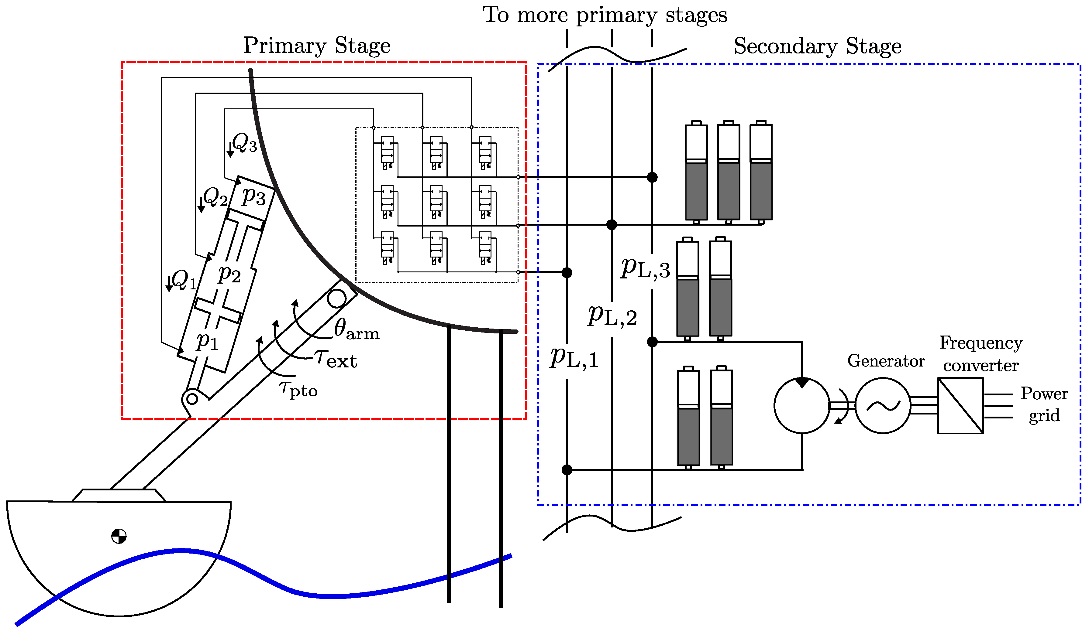
The power take-off topology studied in this paper was proposed for a multiple-point absorber wave energy converter, see [12]. Each absorber is attached to an arm hinged at a fixed structure and in overall terms energy is harvested by the relative motion between the absorber arm and the fixed structure. Figure 1 illustrates the system. Each set of float arm, multi-chamber cylinder and valve manifold constitutes a unit named a primary stage. As indicated in Figure 1, multiple primary stages are connected to a common secondary stage consisting of three pressure lines each equipped with a number of accumulators, a fixed displacement fluid power motor, an electrical generator and a frequency converter for grid connection.

A key advantage of such a topology is that inevitable (but phase shifted) variations in the power production of the individual absorbers do not propagate directly into the secondary stage which in turn leads to a more smooth operation of the fluid power motor and the generator.

It may be noted that the two ports of the fluid power motor are connected to the low ($p_{\mathrm{L},1}$) and high pressure ($p_{\mathrm{L},3}$) lines, respectively. The intermediate pressure ($p_{\mathrm{L},2}$) floats and as detailed in [12] proper secondary control is needed to stabilize this pressure line.

3. Dynamic Modeling

As detailed below, three models are formulated to describe the interconnected dynamics of the incoming wave, the float and the discrete PTO system. The models developed utilize the notation of Figure 1.

3.1. Wave Model

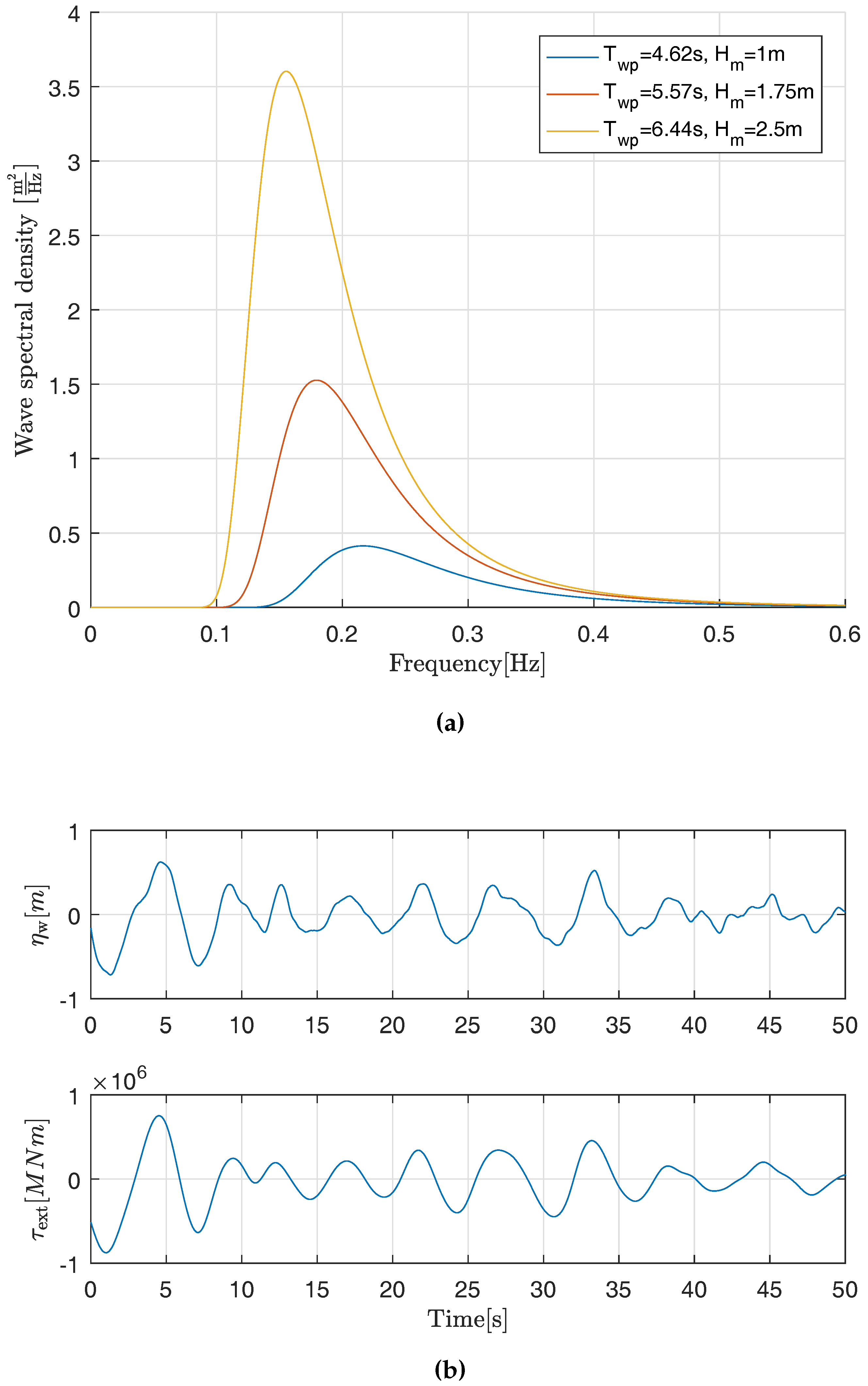
The incoming wave is modeled by the commonly used Pierson-Moskowitz (PM) spectrum for fully developed sea states as described in [14]. The spectrum $S_{\mathrm{PM}}\left(f\right)$ describing the power density versus frequency f is defined by two quantities: the significant wave height, H${}_{\mathrm{m}}$, and the peak wave period, T${}_{\mathrm{wp}}$:

$$S_{\mathrm{PM}}\left(f\right)=\frac{A}{f^5}\exp \left(\frac{-B}{f^4}\right),\mathrm{where}B=\frac{5}{4}\frac{1}{T_{\mathrm{wp}}^4}\mathrm{and}A=\frac{1}{4}B{H}_m^2.$$

(1)

Figure 2a illustrates the wave spectrum for three different sea states that are used for tests throughout the paper.

In our study, the instantaneous wave height ${\eta }_{\mathrm{w}}$ is precomputed in the time domain by filtering Gaussian white noise with unity variance by the PM spectrum as detailed in [12]. In addition, the excitation torque ${\tau }_{\mathrm{ext}}$, defined as the torque applied by the wave on the float fixed in neutral position, is precomputed by filtering the wave height by a force filter with the impulse response $h_{\mathrm{ext}}\left(t\right)$:

$${\tau }_{\mathrm{ext}}\left(t\right)={\int }_{-\infty }^{\infty }{\eta }_{\mathrm{w}}\left(t^{\prime }\right)h_{\mathrm{ext}}(t-t^{\prime })\mathrm{d}{t}^{\prime }$$

(2)

The response $h_{\mathrm{ext}}\left(t\right)$ may be found in [12] based on detailed analysis using the WAMIT tool. For the sea state defined by $T_{\mathrm{wp}}=4.62$ s and ${\mathrm{H}}_{\mathrm{m}}=1$ m, Figure 2b shows examples of wave height and absorber excitation torque.

3.2. Float Model

Based on the work of [2], the float arm motion dynamics are modeled by

$$J_{\mathrm{arm}}{\ddot{\theta }}_{\mathrm{arm}}={\tau }_{\mathrm{res}}+{\tau }_{\mathrm{rad}}+{\tau }_{\mathrm{ext}}+{\tau }_{\mathrm{pto}}$$

(3)

where $J_{\mathrm{arm}}$ is the mass inertia of the float and float arm combined, ${\tau }_{\mathrm{res}}$ is the net restoring torque caused by a combination of Archimedes and gravitational forces, respectively; ${\tau }_{\mathrm{rad}}$ is the radiation torque requested to oscillate the float in clam water and the excitation torque ${\tau }_{\mathrm{ext}}$ is the torque experienced by the float when locked in neutral position and subjected to waves. Finally, ${\tau }_{\mathrm{pto}}$ in (3) denotes the PTO torque acting back on the float.

As explained in [2], the restoring torque may be formulated as ${\tau }_{\mathrm{res}}=k_{\mathrm{res}}{\theta }_{\mathrm{arm}},$ where $k_{\mathrm{res}}$ is constant. The model of the radiation torque is more complex:

$${\tau }_{\mathrm{rad}}\left(t\right)=-J_{\mathrm{add},\infty }{\ddot{\theta }}_{\mathrm{arm}}-\underset{{\tau }_{\mathrm{rad}}^{*}\left(t\right)}{\underbrace{{\int }_0^{\infty }{\omega }_{\mathrm{arm}}\left(t^{\prime }\right)k_{\mathrm{r}}(t-t^{\prime })\mathrm{d}{t}^{\prime }}}$$

(4)

Here, ${\omega }_{\mathrm{arm}}={\dot{\theta }}_{\mathrm{arm}}$ and $k_{\mathrm{r}}\left(t\right)$ is the impulse response for the radiation force which is represented by its Laplace transform by a fifth order transfer function $K_r\left(s\right)$ [2]:

$$K_r\left(s\right)=\frac{{\tau }_{\mathrm{rad}}^{*}\left(s\right)}{{\omega }_{\mathrm{arm}}\left(s\right)}=\frac{b_5{s}^5+\cdots +b_{1}s+b_0}{a_5{s}^5+\cdots +a_{1}s+a_0}.$$

(5)

The first term in (4) describes the torque requested to accelerate the water surrounding the float, given as the added inertia $J_{\mathrm{add},\infty }$ accelerated. As indicated the added inertia is taken as infinite frequency.

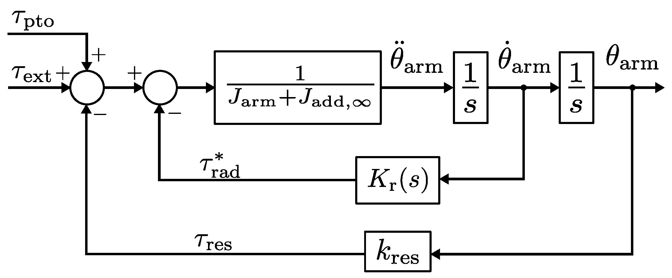
In total, the float dynamics (3) may be represented by the block diagram in Figure 3 or by the input-output transfer function

$$\frac{{\theta }_{arm}\left(s\right)}{{\tau }_{\mathrm{pto}}\left(s\right)+{\tau }_{\mathrm{ext}}\left(s\right)}=\frac{1}{(J_{\mathrm{arm}}+J_{\mathrm{add},\infty })s^2+K_{\mathrm{r}}\left(s\right)s+k_{\mathrm{res}}},$$

(6)

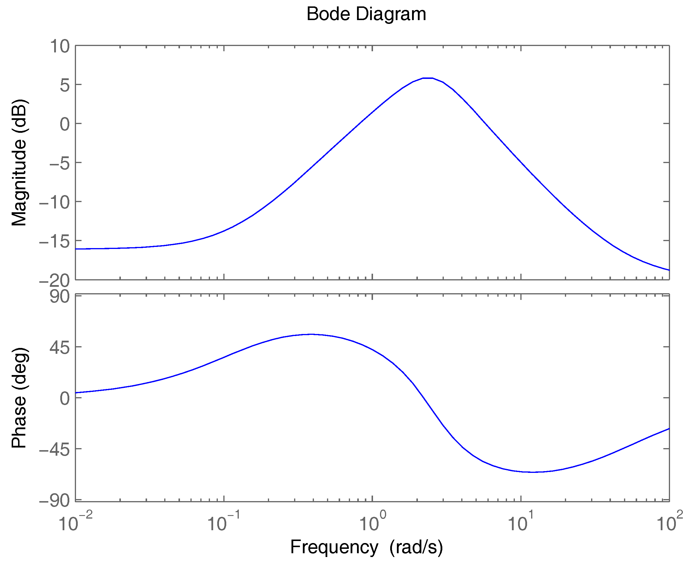
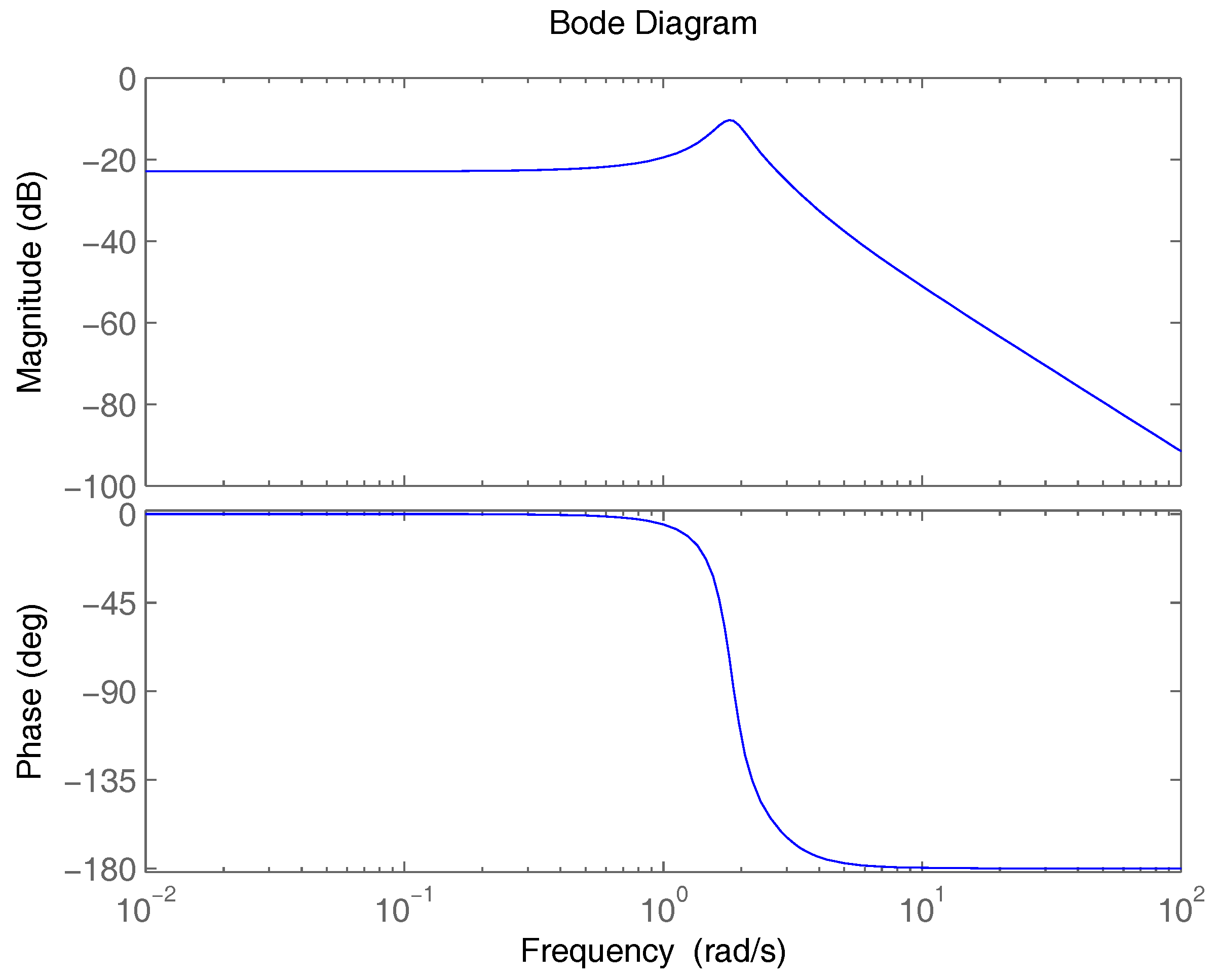
where the frequency response of the radiation gain $K_r\left(s\right)$ is shown in Figure 4 for the system parameters in

Table 1. Float model parameters.

$J_{\mathrm{arm}}$	2.45 $\times {10}^6$	$\left[{\mathrm{kgm}}^2\right]$
$J_{\mathrm{add},\infty }$	1.32 $\times {10}^6$	$\left[{\mathrm{kgm}}^2\right]$
$K_{\mathrm{res}}$	14 $\times {10}^6$	$[\mathrm{Nm}/\mathrm{rad}]$
$[b_5,\cdots ,b_0]$	$[0.01,1.44,62.4,816,1310,144]\times {10}^4$
$[a_5,\cdots ,a_0]$	$[0.0010,0.0906,1.67,6.31,13.3,9.18]$

. A bode diagram of the float model (6) is shown in Figure 5. Note the resonance peak at 0.285Hz indicating the float arm eigen frequency.

3.3. Discrete PTO System Model

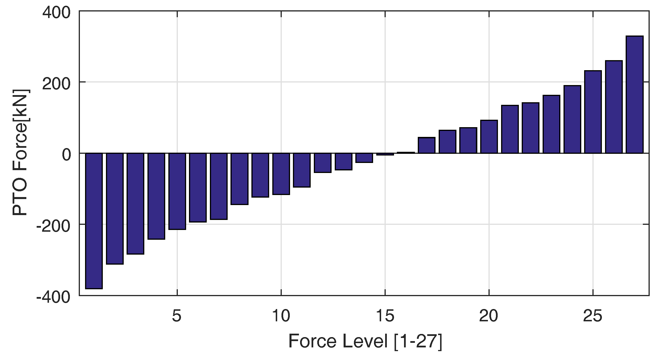
The PTO system consists of a multi chamber cylinder connected to three pressure lines through on/off valves as shown earlier in Figure 1. Using such an arrangement implies that the 27 different PTO force levels shown in Figure 6 can be realized when the configuration data listed in

Table 2. Discrete PTO system parameters. The sign of the areas indicates the force direction.

Chamber Areas	Valve Flow Coef.	Pressure Levels
$A_1=-235$ cm${}^2$	$k_{\mathrm{v},1}=705\frac{\mathrm{l}/\min }{\sqrt{5\mathrm{bar}}}$	$p_{\mathrm{L},1}=20$ bar
$A_2=+122$ cm${}^2$	$k_{\mathrm{v},2}=366\frac{\mathrm{l}/\min }{\sqrt{5\mathrm{bar}}}$	$p_{\mathrm{L},2}=100$ bar
$A_3=+87$ cm${}^2$	$k_{\mathrm{v},3}=261\frac{\mathrm{l}/\min }{\sqrt{5\mathrm{bar}}}$	$p_{\mathrm{L},3}=180$ bar

are used.

The PTO system model consists of a continuity Equation (7) and an orifice Equation (8) for each cylinder chamber:

$$\begin{array}{cc}\hfill {\dot{p}}_i\left(t\right)& =\frac{\beta }{V_i\left(x_{\mathrm{c}}\left(t\right)\right)}\left(Q_i\left(t\right)+A_i{\dot{x}}_{\mathrm{c}}\left(t\right)\right)\hfill \end{array}$$

(7)

$$\begin{array}{cc}\hfill Q_i\left(t\right)& ={\Sigma }_{j=1}^3{k}_{\mathrm{v},i}{x}_{i,j}\sqrt{|p_{\mathrm{L},j}-p_i\left(t\right)|}\mathrm{sign}(p_{\mathrm{L},j}-p_i\left(t\right))\hfill \end{array}$$

(8)

Here, $p_i\left(t\right)$ is the pressure in chamber i and the flow into the chamber is $Q_i$. The ith piston area and chamber volume are denoted by $A_i$ and $V_i$, respectively. $x_{\mathrm{c}}$ is the piston position. $x_{i,j}$ is the normalised valve opening from the jth pressure line to the i’th cylinder chamber and $k_{\mathrm{v},i}$ is the valve flow coefficient. $p_{\mathrm{L},j}$ is the jth line pressure. In the analysis, bulk modulus is set constant to $\beta =8000$ bar.

The valves are matched to the chambers they are connected to and by proper pairing the pressure drop across the valves are 5 bar for a piston velocity of 0.5 m/s.

The total PTO force $F_{\mathrm{pto}}\left(t\right)$ then becomes:

$$F_{\mathrm{pto}}\left(t\right)=\sum _{i=1}^3{A}_i{p}_i\left(t\right)$$

(9)

4. Model Predictive Control of Discrete PTO System

In the context of a PTO system, the overall control problem is to maximize the energy output in (varying) sea states by clever manipulation of the PTO force, which in our case must be selected from a pool of 27 values. Traditionally, a controller is tuned off-line based on ideas such as reactive control [2] and mapping techniques are used to accommodate quantization of the controller output [12].

As an alternative to such an indirect approach, to attack both the energy maximization problem and the force level quantization problem, the variant of closed-loop control model known as either receding horizon control or model predictive control has two appealing characteristics for use in a WEC with a discrete PTO system: as detailed in [15], MPC allows direct handling of constraints such as actuator and state limitations—and also, due to the use of an on-line optimization strategy, MPC should be able to address the energy maximization problem directly during runtime.

The overall idea of MPC is to compute the future controller outputs (i.e., the system inputs) by solving an optimizing problem on each time step of duration $T_{\mathrm{S}}$. More specifically, the strategy for a discrete-time MPC involves three steps:

• Measure (or partially estimate) the full system state $x\left(k\right)$ at the current sampling time $t\left(k\right)$.
• Find the N optimal future system inputs

  $$\begin{array}{c}\hfill {\mathcal{U}}_k=[u\left(k\right),u(k+1),\cdots u(k+N-1)]\end{array}$$

  (10)

  by solving an optimization problem over a finite time horizon $T_{\mathrm{H}}=NT{}_{\mathrm{s}}$ by using a prediction model to estimate the future system states

  $$\begin{array}{c}\hfill {\mathcal{X}}_k=[x(k+1),x(k+2),\cdots x(k+N)]\end{array}$$

  (11)

  based on the initial state $x\left(k\right)$, the future inputs ${\mathcal{U}}_k$ besides a prior estimates of future disturbances
• Apply only the first optimal controller output $u\left(k\right)$ to the system and loop back to step 1 for the next sampling instant.

Figure 7 illustrates the used notation and the MPC principle: at time $t\left(k\right)$ the actual state $x\left(k\right)$ is available and an optimal future controller output vector ${\mathcal{U}}_k$ is determined as outline in Step 2 above. Using ${\mathcal{U}}_k,$ the predicted future state becomes ${\mathcal{X}}_k$ as shown in the bottom part of Figure 7. The first element $u\left(k\right)$ is immediately applied to the system and as indicated the actual state trajectory may deviate from the prediction leading to another initial state in the next sampling interval starting at $t(k+1)=t\left(k\right)+T_{\mathrm{s}}$.

In the following subsections, the configuration of the MPC based WPEA is described in detail.

4.1. Prediction Model

Denoting the total input as $\tilde{u}=u+w\triangleq {\tau }_{\mathrm{pto}}+{\tau }_{\mathrm{ext}},$ the prediction model is the float model in (6) represented in continuous-time state space as

$$\begin{array}{c}\begin{array}{cc}\hfill \left[\begin{array}{c}{\ddot{\theta }}_{arm}\\ {\dot{\theta }}_{arm}\\ {\dot{\tau }}_{\mathrm{rad},\mathrm{kr}}\\ {\dot{x}}_{kr,1}\\ {\dot{x}}_{kr,2}\\ {\dot{x}}_{kr,3}\\ {\dot{x}}_{kr,4}\end{array}\right]& =\left[\begin{array}{ccccccc}0& \frac{-k_{res}}{J_{tot}+J_{tot}}& \frac{-1}{J_{tot}+J_{tot}}& 0& 0& 0& 0\\ 1& 0& 0& 0& 0& 0& 0\\ b_1-a_1{b}_0& 1& -a_1& 1& 0& 0& 0\\ b_2-a_2{b}_0& 1& -a_2& 0& 1& 0& 0\\ b_3-a_3{b}_0& 1& -a_3& 0& 0& 1& 0\\ b_4-a_4{b}_0& 1& -a_4& 0& 0& 0& 1\\ b_5-a_5{b}_0& 1& -a_5& 0& 0& 0& 0\end{array}\right]\left[\begin{array}{c}{\dot{\theta }}_{arm}\\ {\theta }_{arm}\\ {\tau }_{\mathrm{rad},\mathrm{kr}}\\ x_{kr,1}\\ x_{kr,2}\\ x_{kr,3}\\ x_{kr,4}\end{array}\right]+\left[\begin{array}{c}\frac{-1}{J_{tot}+J_{tot}}\\ 0\\ 0\\ 0\\ 0\\ 0\\ 0\end{array}\right]\tilde{u}\hfill \\ \hfill {\dot{\theta }}_{\mathrm{arm}}& =\left[\begin{array}{cccc}1& 0& \cdots & 0\end{array}\right]{\left[\begin{array}{ccccccc}{\dot{\theta }}_{arm}& {\theta }_{arm}& {\tau }_{\mathrm{rad},\mathrm{kr}}& x_{kr,1}& x_{kr,2}& x_{kr,3}& x_{kr,4}\end{array}\right]}^T\hfill \end{array}\end{array}$$

(12)

It may be noted that the PTO system dynamics are not included in (12) i.e., infinitely fast force development is assumed because the MPC sample time is significantly higher than the force rise time. The prediction of future states are based on a discrete state space model of the float dynamics (12):

$$\begin{array}{cc}\hfill x(k+1)& =Ax\left(k\right)+B\tilde{u}\left(k\right)\hfill \\ & =Ax\left(k\right)+B\left(u\left(k\right)+w\left(k\right)\right)\hfill \\ \hfill y\left(k\right)& =Cx\left(k\right),\hfill \end{array}$$

(13)

where $u\left(k\right)$ relates to controllable input (${\tau }_{\mathrm{pto}}$) and $w\left(k\right)$ is the uncontrollable disturbance (${\tau }_{\mathrm{ext}}$). In addition, A, B and C are the discrete representation of the system matrices of (12) using a zero order hold discretization with the sample time equal to $T_{\mathrm{S}}$. The angular velocity of the float arm is set to be the system output. By using (13) recursively, the future states in the prediction horizon may be expressed by the system matrices, the initial state and the future system inputs ${\mathcal{U}}_k$ and disturbances ${\mathcal{W}}_k$ as:

$$\begin{array}{cc}\hfill \underset{{\mathcal{X}}_k}{\underbrace{\left[\begin{array}{c}x(k+1)\\ x(k+2)\\ ⋮\\ x(k+N)\end{array}\right]}}=\underset{\mathrm{P}}{\underbrace{\left[\begin{array}{c}A\\ A^2\\ ⋮\\ A^N\end{array}\right]}}x\left(k\right)& +\underset{\mathrm{H}}{\underbrace{\left[\begin{array}{cccc}B& 0& \cdots & 0\\ AB& B& \cdots & 0\\ ⋮& ⋮& \ddots & ⋮\\ A^{N-1}B& A^{N-2}B& \cdots & B\end{array}\right]}}\underset{{\mathcal{U}}_k}{\underbrace{\left[\begin{array}{c}u\left(k\right)\\ u(k+1)\\ ⋮\\ u(k+N-1)\end{array}\right]}}\hfill \\ & +\left[\begin{array}{cccc}B& 0& \cdots & 0\\ AB& B& \cdots & 0\\ ⋮& ⋮& \ddots & ⋮\\ A^{N-1}B& A^{N-2}B& \cdots & B\end{array}\right]\underset{{\mathcal{W}}_k}{\underbrace{\left[\begin{array}{c}w\left(k\right)\\ w(k+1)\\ ⋮\\ w(k+N-1)\end{array}\right]}}\hfill \end{array}$$

(14)

The future system outputs ${\mathcal{Y}}_k$ may be stated as:

$$\underset{{\mathcal{Y}}_k}{\underbrace{\left[\begin{array}{c}y(k+1)\\ y(k+2)\\ ⋮\\ y(k+N)\end{array}\right]}}=\underset{{\mathrm{C}}_{\omega }}{\underbrace{\left[\begin{array}{cccc}C& 0& \cdots & 0\\ 0& C& \cdots & 0\\ ⋮& ⋮& \ddots & ⋮\\ 0& 0& \cdots & C\end{array}\right]}}{\mathcal{X}}_k$$

(15)

By decomposing the total system input into the excitation torque and the torque applied by the PTO system, the future states may be reformulated as

$${\mathcal{X}}_k=\mathrm{P}x\left(k\right)+\mathrm{H}{\mathcal{T}}_{k,\mathrm{ext}}+\mathrm{H}{\mathcal{T}}_{k,\mathrm{pto}}.$$

(16)

Hence, (16) related the future states ${\mathcal{X}}_k$ to the initial state $x\left(k\right)$ at time $t\left(k\right)$ and to the controller output vector ${\mathcal{T}}_{k,\mathrm{pto}}$ under the assumption that the disturbance ${\mathcal{T}}_{k,\mathrm{ext}}$ are known in the whole time horizon $T_{\mathrm{H}}$.

4.2. MPC Objective Functions

The main task is to maximize the absorbed PTO energy. Using (15) and (16), the total energy $E_{\mathrm{abs}}$ absorbed during the prediction horizon $N{T}_s$ may be approximated by backward Euler integration of the instantaneous power:

$$E_{\mathrm{abs}}={\int }_{t\left(k\right)}^{t\left(k\right)+N{T}_s}{\dot{\theta }}_{\mathrm{arm}}\left(t\right){\tau }_{\mathrm{pto}}\left(t\right)\mathrm{d}t\approx T_s{\mathcal{Y}}_k^T{\mathcal{T}}_{k,\mathrm{pto}}$$

(17)

where it may be recalled that ${\mathcal{Y}}_k$ is a function of ${\mathcal{T}}_{k,\mathrm{pto}}.$ The objective function to be maximized is defined as

$$\begin{array}{c}{J}_1=E_{\mathrm{abs}}\hfill \end{array}$$

(18)

and the optimization problem is then formulated as

$$\begin{array}{c}\hfill \underset{{\mathcal{T}}_{k,\mathrm{pto}}}{max}{J}_1\end{array}$$

(19)

subjected to the constraints that all elements in ${\mathcal{T}}_{k,\mathrm{pto}}=[{\tau }_{\mathrm{pto}}\left(k\right),{\tau }_{\mathrm{pto}}(k+1),\cdots ,{\tau }_{\mathrm{pto}}(k+N-1)]$ must belong to the set of 27 possible values dictated by the discrete PTO system. The optimization problem is solved by a differential evolution algorithm originating from the work of [16] and refined in e.g., [17].

As part of the initial feasibility study of MPC for PTO systems, a force-continuous MPC version has been studied, where the allowable forces are not constrained to a discrete set. Instead, a simple bound ${\tau }_{\mathrm{pto},\min }\le {\tau }_{\mathrm{pto}}\left(k\right)\le {\tau }_{\mathrm{pto},\max }$ for any k is adopted. In this continuous case the optimization problem may be solved by standard quadratic methods, by rephrasing the absorbed power (17) into a quadratic form:

$$E_{\mathrm{abs}}\left({\tau }_{\mathrm{pto}}\right)=-T_s\left({\mathcal{T}}_{k,\mathrm{pto}}^{T}Q{\mathcal{T}}_{k,\mathrm{pto}}-f{\mathcal{T}}_{k,\mathrm{pto}}\right),$$

(20)

where $Q=H^T{C}_{\omega }^T$ and $f={\mathcal{X}}_k^T{P}^T{C}_{\omega }^T+{\mathcal{T}}_{k,\mathrm{ext}}^T{H}^T{C}_{\omega }^T$.

4.3. MPC Objective Functions—Included Losses

The problem (19) does not take the system losses into account which may lead to suboptimal performance from an energy harvesting point of view. As elaborated in the next subsection, the two main loss phenomena are (i) losses $E_{\mathrm{loss},\mathrm{s}}$ associated with shifting of the PTO force from one level to another and (ii) throttling losses $E_{\mathrm{loss},\mathrm{t}}$. Therefore, two alternative MPC strategies are investigated based on the objective functions

$$\begin{array}{c}{J}_2=E_{\mathrm{abs}}-E_{\mathrm{loss},\mathrm{s}}\hfill \end{array}$$

(21)

$$\begin{array}{c}{J}_3=E_{\mathrm{abs}}-E_{\mathrm{loss},\mathrm{s}}-E_{\mathrm{loss},\mathrm{t}}\hfill \end{array}$$

(22)

The three outlined MPC strategies are compared in Section 5 once loss models have been established below.

4.4. Loss Models

The losses in the primary stages of the PTO system may be separated into three parts: mechanical friction in the PTO cylinder, loss associated with shifting the pressure inside each cylinder chamber and throttling losses associated with the displacement flow. In the current work, the mechanical friction in the PTO is neglected. The energy loss associated with shifting the chamber pressure from one value to another by switching the chamber to a new pressure line through a valve was analyzed in [18] and this work is used as a starting point for the loss models introduced below.

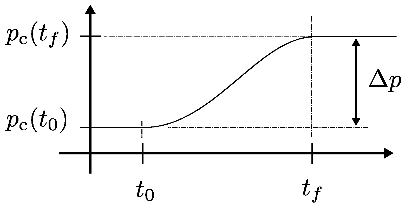
A pressure shift is performed by controlling the valve during the shifting time $T_{\mathrm{p}}=t_f-t_0$ such a third order chamber pressure profile appears as illustrated in Figure 8. The cylinder volume rate of change is assumed constant during the pressure shifting time such that

$$\begin{array}{c}\hfill {\dot{V}}_{\mathrm{c}}\left(t\right)={\dot{V}}_{\mathrm{c}}\left(t_0\right)\mathrm{for}{t}_0\le t\le t_f\end{array}$$

(23)

i.e., the piston velocity is assumed constant during the pressure shifting time $T_{\mathrm{p}}$.

The energy loss for a pressure shift of $\Delta p$ is in [18] shown to be:

$$E(\Delta p)=\frac{1}{2}\left(\frac{\Delta p^2}{\beta }{V}_{\mathrm{c}}\left(t_0\right)+\Delta p{\dot{V}}_{\mathrm{c}}\left(t_0\right)T_{\mathrm{p}}\right)+\frac{13}{70}\frac{\Delta p^2}{\beta }{\dot{V}}_{\mathrm{c}}\left(t_0\right)T_{\mathrm{p}}$$

(24)

To include the shifting losses in the MPC objective functions it should be stated as a function of the quantized force levels. Using (24) for all three chambers, the total shifting loss in the prediction horizon $N{T}_s$ may then be stated as:

$$\begin{array}{cc}\hfill E_{\mathrm{loss},\mathrm{s}}=\sum _{i=1}^3\sum _{n=1}^N& \left[\frac{1}{2}\left(\frac{{\left(p_{i,n}-p_{i,n-1}\right)}^2}{\beta }{V}_{\mathrm{c},i,n}+\left(p_{i,n}-p_{i,n-1}\right){\dot{V}}_{\mathrm{c},i,n}{T}_{\mathrm{p}}\right)\right.\hfill \\ \hfill & \left.+\frac{13}{70}\frac{{\left(p_{i,n}-p_{i,n-1}\right)}^2}{\beta }{\dot{V}}_{\mathrm{c},i,n}{T}_{\mathrm{p}}\right],\hfill \end{array}$$

(25)

where $p_{i,n}$ is the pressure in the i’th chamber at time instant n found using a lookup table mapping the force level to corresponding chamber pressures. In addition, in (25) $V_{\mathrm{c},i,n}$ is the ith chamber volume in the nth prediction step. $V_{\mathrm{c},i,n}$ relates geometrically to the arm angle ${\theta }_{\mathrm{arm}}$ as seen in Figure 1.

To calculate the steady state throttle losses, it may be noted that for each chamber $i\in \{1,2,3\}$, three valves are used to connect to the low, medium, and high pressure lines, respectively. In practice the three valves belonging to the same pressure chamber are identical i.e., these three valves all have the same flow coefficient labeled $k_{\mathrm{v},i}$. Knowing the flow into the ith chamber, the throttling power losses associated with that flow is $Q_i^3/k_{\mathrm{v},i}^2$, independently of which pressure line the chamber is connected to. The total throttle loss for all chambers may thus be expressed as

$$P_{\mathrm{loss},\mathrm{t}}=\sum _{i=1}^3\frac{Q_i^3}{k_{\mathrm{v},i}^2}={\dot{x}}_{\mathrm{c}}^3\sum _{i=1}^3\frac{A_i^3}{k_{\mathrm{v},i}^2}\triangleq k_t{\dot{x}}_{\mathrm{c}}^3,$$

(26)

where $k_{\mathrm{t}}$ defines the total loss coefficient. Table 2 lists the chamber areas $A_i$ and flow coefficients $k_{\mathrm{v},i}$.

Using a backward Euler approximation, the total throttle energy loss in the whole prediction horizon may now be calculated by

$$E_{\mathrm{loss},\mathrm{t}}={\int }_{t\left(k\right)}^{t\left(k\right)+N{T}_s}{k}_{\mathrm{t}}{\dot{x}}_{\mathrm{c}}^3\mathrm{d}t\approx k_{\mathrm{t}}{T}_{\mathrm{s}}\sum _{n=1}^N{\dot{x}}_{c,n}^3,$$

(27)

where ${\dot{x}}_{c,n}$ is the piston velocity in the nth prediction step. Note that ${\dot{x}}_{c,n}$ may be calculated straightforwardly once the arm angular velocity ${\dot{\theta }}_{\mathrm{arm}}$ has been calculated by the prediction model when the geometry (Figure 1) is known.

5. Results

As detailed in Section 4, three different MPC objective functions have been formulated for the discrete PTO system described in Section 2. To establish a baseline for evaluation of these MPC strategies, the reactive control algorithm described in the first subsection below is used. Next, to investigate the impact of the MPC prediction horizon $T_{\mathrm{H}}$ and the time step $T_{\mathrm{S}}$ on the absorbed power, the force-continuous version of MPC described in Section 4.2 is used for an initial analysis. Finally, a series of comparisons between the three discrete MPC controllers are reported.

5.1. Discrete Reactive Control

For MPC benchmarking the reactive control algorithm developed in [12] is used. The PTO torque controller is

$${\tau }_{\mathrm{pto}}=B{\dot{\theta }}_{\mathrm{arm}}+K{\theta }_{\mathrm{arm}},$$

(28)

which basically imposes a PTO force in phase with the velocity of the absorber’s arm besides a damping term. Equation (28) gives a continuous torque command, which is translated into one of the applicable quantized force levels by the force shifting algorithm also described in [12]. This force shifting algorithm is based on an off-line optimization where the force step associated with lowest energy loss is chosen while restraining the force error imposed by the quantization of the PTO force. In addition, the controller coefficients B and K in (28) are optimized for each sea state to maximize the absorbed energy. In total, this reactive controller has proven to be quite efficient on a full-scale WEC [12].

5.2. Methodology

The assessment of the various WPEA strategies is based on post-processing of the time-domain response of the wave energy converter using the dynamic models of the wave dynamics, the float and PTO system described in Section 3.

Specifically, the benchmarking is based on calculation of the average absorbed power and average harvested power during an observation interval T:

$$\begin{array}{cc}\hfill P_{\mathrm{abs}}& =\frac{1}{T}{\int }_0^T{\dot{\theta }}_{\mathrm{arm}}\left(t\right){\tau }_{\mathrm{pto}}\left(t\right)\mathrm{d}t\hfill \end{array}$$

(29)

$$\begin{array}{cc}\hfill P_{\mathrm{har}}& =\frac{1}{T}{\int }_0^T\sum _{j=1}^3{p}_{L,j}{Q}_j\left(t\right)\mathrm{d}t,\hfill \end{array}$$

(30)

where $p_{L,j}$ denotes the pressure on pressure line j.

It may be noted that $P_{\mathrm{har}}$ is the net hydraulic power delivered from the primary stage to the secondary stage. The PTO conversion efficiency is ${\eta }_{\mathrm{pto}}=P_{\mathrm{har}}/P_{\mathrm{abs}}.$

Using the three wave conditions shown in Figure 2, $P_{\mathrm{abs}}$, $P_{\mathrm{har}}$ and $\eta$ are calculated for the different control strategies.

5.3. MPC Time Step and Prediction Horizon Analysis

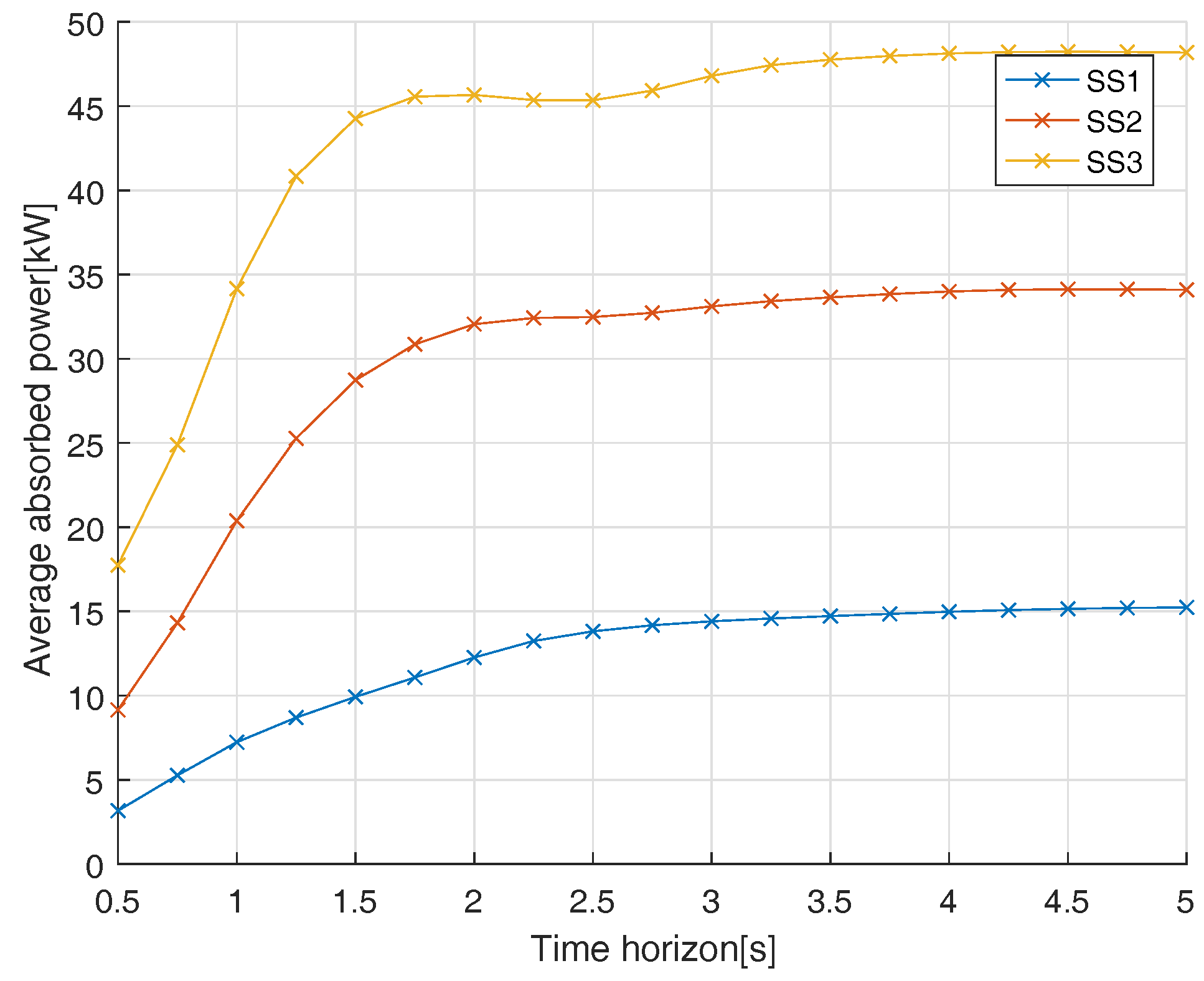
To investigate the overall influence of time step and prediction horizon, both parameters are varied separately and the absorbed power is determined. Neglecting the PTO dynamics and losses, and using the force-continuous MPC (Section 4.2), the results shown in Figure 9 and Figure 10 are obtained for the three different sea states.

Using a very small time step ($T_{\mathrm{s}}$ = 25 ms) , Figure 9 shows for all sea states that the average absorbed power increases when the prediction horizon is increased. In addition, the results indicate that the absorbed power flattens and nothing is gained by increasing the prediction horizon beyond 5 s. Keeping the prediction horizon fixed at $T_{\mathrm{H}}=5$ s, Figure 10 shows that the average absorbed power decreases when increasing the time step leading to the conclusion that the time step should be as low as possible. In addition, the lower sea states ideally require smaller time steps because the relative change of $P_{\mathrm{abs}}$ versus $T_{\mathrm{s}}$ increases when the peak wave period is reduced.

5.4. MPC and Reactive Control Performance Analysis

The three MPC objective functions for a discrete PTO system introduced in Section 4.2 and Section 4.3 are labeled as

MPC${}_1$:

$J_1=E_{\mathrm{abs}}$ (18)

MPC${}_2$:

$J_2=E_{\mathrm{abs}}-E_{\mathrm{loss},\mathrm{s}}$ (21)

MPC${}_3$:

$J_3=E_{\mathrm{abs}}-E_{\mathrm{loss},\mathrm{s}}-E_{\mathrm{loss},\mathrm{t}}$ (22)

In addition, the label ’Reactive’ is used for the baseline controller discussed in Section 5.1.

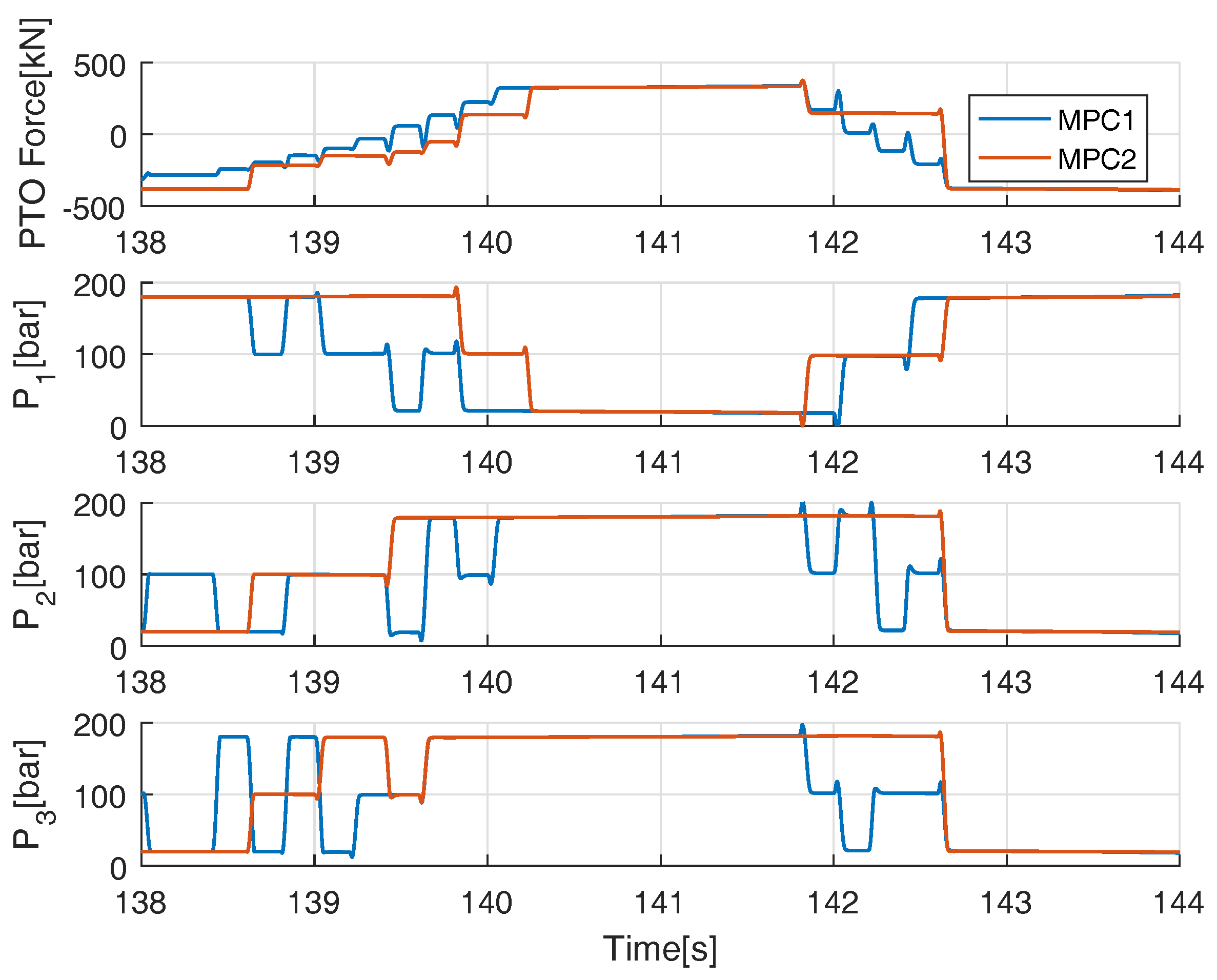
To illustrate the time domain waveforms, Figure 11 shows the PTO force and the three chamber pressures using MPC${}_1$ and MPC${}_2$, respectively. It is seen that MPC${}_1$ leads to many more pressure shifts than MPC${}_2$ and as summarized later the many switchings associated with MPC${}_1$ reduces the harvested power significantly.

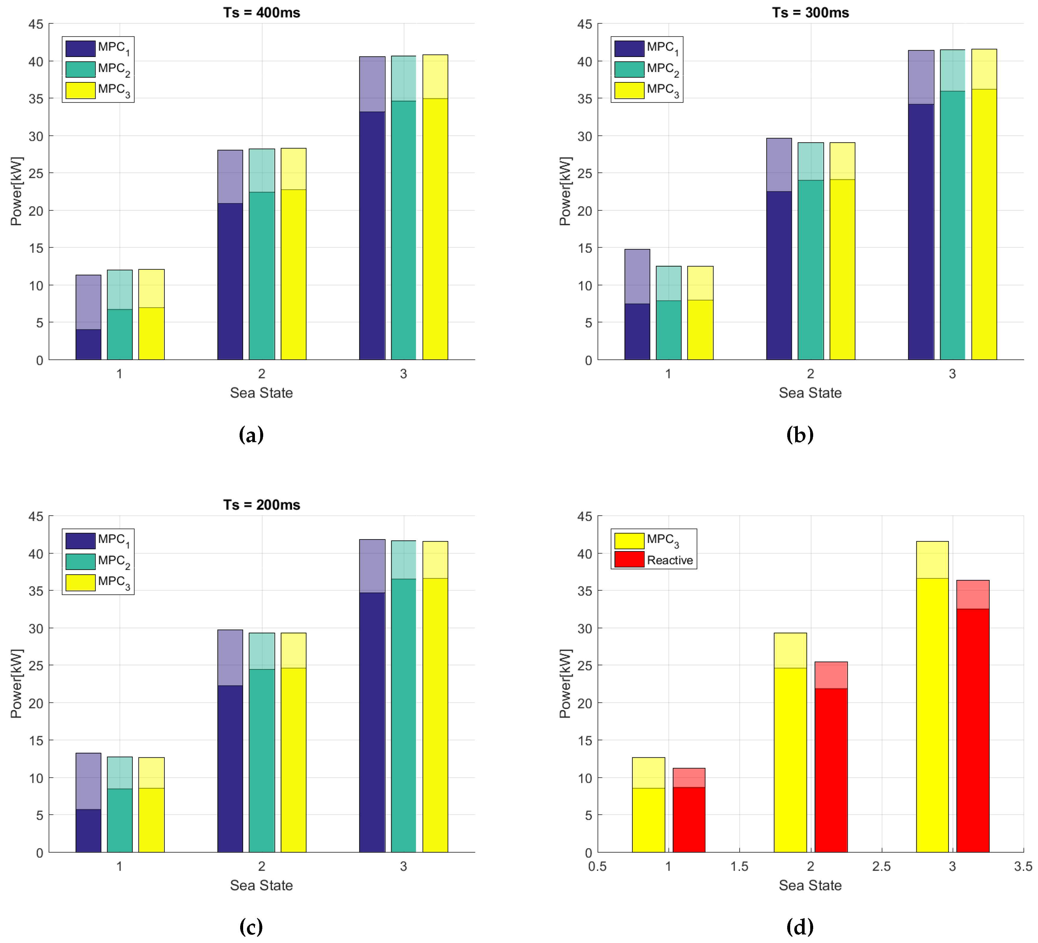
In Figure 12 the average $P_{\mathrm{abs}}$ absorbed and harvested $P_{\mathrm{har}}$ power are shown for the three sea states for each of the different controllers. These results have been computed using a 5 s prediction horizon for three values of the sampling time i.e., $T_{\mathrm{s}}\in \{200,300,400\}$ ms. According to the preliminary findings in Section 5.3, $T_{\mathrm{s}}$ should be as small as possible, but in the detailed analysis that includes losses, it has been found that $T_{\mathrm{s}}=200$ ms is a good compromise that ensures that the pressure dynamics associated with the switchings have time to settle before a shift to a new force level is initialed. Referring to Section 4.4, the shifting time $T_{\mathrm{p}}$ may be in the order of 50 ms for the PTO system used in this investigation [12].

In

Table 3. Average absorbed power, harvested power and efficiency for three different sea states for different WPEAs.

	Absorbed Power (kW)			Harvested Power (kW)			Efficiency (-)
Sea State	1	2	3	1	2	3	1	2	3
MPC${}_1$	13.14	29.63	42.02	6.11	22.33	34.71	0.47	0.75	0.86
MPC${}_2$	12.48	29.53	42.00	9.10	25.39	37.43	0.73	0.86	0.89
MPC${}_3$	12.32	29.37	41.65	9.15	25.48	37.43	0.74	0.87	0.90
Reactive	11.23	25.41	36.36	8.68	21.86	32.52	0.77	0.86	0.89

the average absorbed power $P_{\mathrm{abs}}$, the average harvested power $P_{\mathrm{har}}$ and the PTO efficiency $\eta$ in the three sea states are tabulated for MPC${}_1$, MPC${}_2$, and MPC${}_3$ using $T_{\mathrm{s}}=200$ ms besides the reactive baseline controller. In general, the MPC controllers are seen to perform better than the reactive WPEA. Furthermore, it may be seen that MPC${}_2$ inclusion of the shifting losses in the objective function increases the harvested power significantly whereas MPC${}_3$ that also includes throttling losses does not contribute to any gain in the harvested power.

When comparing the results in Table 3 for the MPC${}_2$ and the reactive WPEAs, it may be noted that the PTO system efficiency is a poor performance indicator: these two controllers yield the same efficiency in sea state 2, even though harvested power differs a lot. On the other hand, the efficiency may indicate wear on the system as energy is dissipated in the PTO system.

6. Conclusions

The study presented in this paper clearly indicates that a MPC based WPEA is capable of improving the energy output of a WEC using a discrete fluid power PTO system. Especially, it is concluded that the inclusion of energy losses in the conversion system is of utmost importance because the optimal PTO force depends highly on the PTO system losses.

Under the assumption that incoming wave is known, the MPC algorithm excels compared to the reactive algorithm with its ability to adapt on-line to the incoming irregular waves and the inherent inclusion of the quantized PTO system.

The investigation points out that a step time as short as possible is preferable whereas a prediction horizon above 5 s seems futile.

In conclusion, model predictive control based wave power extraction algorithms appear favorable for wave energy converters utilizing discrete fluid power PTO system. Future research is directed toward the practical real-time implementation of MPC, including studies of model complexity reductions and optimization algorithm implementation. This will be investigated using the test facility described in [19,20]. Furthermore, the required accuracy of the wave prediction algorithm is a topic of great importance.

References

- Drew, B.; Plummer, A.R.; Sahinkaya, M.N. A review of wave energy converter technology. Proc. Inst. Mech. Eng. Part A 2016, 223, 887–902. [Google Scholar] [CrossRef]
- Hansen, R.H.; Kramer, M.M. Modelling and control of the Wavestar prototype. In Proceedings of the 9th European Wave and Tidal Energy Conference (EWTEC), Southampton, UK, 5–9 September 2011. [Google Scholar]
- Hansen, A.H.; Pedersen, H.C. Optimal discrete PTO force point absorber wave energy converters in regular waves. In Proceedings of the 10th European Wave and Tidal Energy Conference (EWTEC), Southampton, UK, 5–9 September 2013. [Google Scholar]
- Cretel, J.A.; Lightbody, G.; Thomas, G.P.; Lewis, A.W. Maximisation of energy capture by a wave-energy point absorber using model predictive control. IFAC Proc. 2011, 44, 3714–3721. [Google Scholar] [CrossRef]
- Richter, M.; Magana, M.E.; Sawodny, O.; Brekken, T.K. Nonlinear model predictive control of a point absorber wave energy converter. IEEE Trans. Sustain. Energy 2013, 4, 118–129. [Google Scholar] [CrossRef]
- Soltani, M.N.; Sichani, M.T.; Mirzaei, M. Model predictive control of buoy type wave energy converter. In Proceedings of the 19th World Congress of the International Federation of Automatic Control, Cape Town, South Africa, 24–29 August 2014. [Google Scholar]
- Andersen, P.; Pedersen, T.S.; Nielsen, K.M.; Vidal, E. Model predictive control of a wave energy converter. In Proceedings of the 2015 IEEE Conference on Control Applications (CCA), Sydney, Australia, 21–23 September 2015; pp. 1540–1545. [Google Scholar] [CrossRef]
- Cretel, J.; Lewis, A.W.; Lightbody, G.; Thomas, G.P. An application of model predictive control to a wave energy point absorber. IFAC Proc. Vol. 2010, 43, 267–272. [Google Scholar] [CrossRef]
- Hendrikx, R.W.M.; Leth, J.; Andersen, P.; Heemels, W.P.M.H. Optimal control of a wave energy converter. In Proceedings of the 2017 IEEE Conference on Control Technology and Applications (CCTA), Kohala Coast, HI, USA, 27–30 August 2017; pp. 779–786. [Google Scholar] [CrossRef]
- Oetinger, D.; Magaña, M.E.; Sawodny, O. Decentralized Model predictive control for wave energy converter arrays. IEEE Trans. Sustain. Energy 2014, 5, 1099–1107. [Google Scholar] [CrossRef]
- Tom, N.; Yeung, R.W. Non-linear model predictive control applied to a generic ocean-wave energy extractor. In Proceedings of the AMSE 32nd International Conference on Ocean, Offshore and Arctic Engineering, Nantes, France, 9–14 June 2013. [Google Scholar] [CrossRef]
- Hansen, R.H.; Kramer, M.M.; Vidal, E. Discrete displacement hydraulic power take-off system for the Wavestar wave energy converter. Energies 2013, 6, 4001–4044. [Google Scholar] [CrossRef]
- Kramer, M.; Marquis, L.; Frigaard, P. Performance evaluation of the Wavestar prototype. In Proceedings of the 9th European Wave and Tidal Conference (EWTEC), Southampton, UK, 5–9 September 2011. [Google Scholar]
- Falnes, J. Ocean Waves and Oscillating Systems: Linear Interactions Including Wave-Energy Extraction; Cambridge University Press: Cambridge, UK, 2002. [Google Scholar] [CrossRef]
- Dai, L.; Xia, Y.; Fu, M.; Mahmoud, M.S. Discrete-time model predictive control. In Advances in Discrete Time Systems; Mahmoud, M., Ed.; InTech: Rijeka, Croatia, 2012. [Google Scholar] [CrossRef]
- Storn, R.; Price, K. Differential Evolution—A Simple and Efficient Adaptive Scheme for Global Optimization over Continuous Spaces; Tech. Report TR-95-012; Berkeley: Cambridge, MA, USA, 1995. [Google Scholar]
- Kukkonen, S. Generalized Differential Evolution for Global Multi-Objective Optimization with Constraints. Ph.D. Thesis, Lappeenranta University of Technology, Lappeenranta, Finland, 2012. [Google Scholar]
- Hansen, A.H.; Pedersen, H.C. Reducing pressure oscillations in discrete fluid power systems. Inst. Mech. Eng. Proc. Part I 2016, 230, 1093–1105. [Google Scholar] [CrossRef]
- Hansen, A.H.; Pedersen, H.C.; Hansen, R.H. Validation of simulation model for full scale wave simulator and discrete fluid power PTO system. In Proceedings of the 9th JFPS International Symposium on Fluid Power, Matsue, Japan, 28–31 October 2014. [Google Scholar]
- Pedersen, H.C.; Hansen, R.H.; Hansen, A.H.; Andersen, T.O.; Bech, M.M. Design of full scale wave simulator for testing Power Take Off systems for wave energy converters. Int. J. Mar. Energy 2016, 13, 130–156. [Google Scholar] [CrossRef]
Figure 1.
WEC with multiple point absorbers based on a discrete PTO system.
Figure 2.
Sea state model: (a) Pierson-Moskowitz spectrum for three sea states and (b) example of wave height and excitation torque in time domain for s and m.
Figure 3.
Block diagram of the float model.
Figure 4.
Bode diagram of the radiation damping term (5) normalized to 1 MNm/(rad/s).
Figure 5.
Bode diagram of the float dynamics (6) normalized to 1 rad/MNm.
Figure 6.
Applicable static force levels for the discrete PTO system.
Figure 7.
MPC notation and principles. (Top) controller output and (bottom) system states.
Figure 8.
Illustration of pressure shift in a single cylinder chamber.
Figure 9.
Average absorbed power versus prediction horizon for a 25 ms time step for three sea states.
Figure 10.
Average absorbed power versus time step for 5 s prediction horizon for three sea states.
Figure 11.
Examples of PTO force and chamber pressures for MPC and MPC using ms.
Figure 12.
Average absorbed and harvested power versus sea states using different controllers. (a) = 400 ms; (b) = 300 ms; (c) = 200 ms; (d) Reactive controller versus MPC.