A Multi-Parameter Optimization Model for the Evaluation of Shale Gas Recovery Enhancement


1
State Key Laboratory for Geomechanics & Deep Underground Engineering, China University of Mining and Technology, Xuzhou 221116, China
2
Center for Offshore Research and Engineering, National University of Singapore, E1A-07-03, 1 Engineering Drive 2, Singapore 117576, Singapore
3
School of Mechanics and Civil Engineering, China University of Mining and Technology, Xuzhou 221116, China
*
Author to whom correspondence should be addressed.
Energies 2018, 11(3), 654; https://doi.org/10.3390/en11030654
Submission received: 14 February 2018
/
Revised: 7 March 2018
/
Accepted: 9 March 2018
/
Published: 15 March 2018
(This article belongs to the Section L: Energy Sources)
Abstract
:Although a multi-stage hydraulically fractured horizontal well in a shale reservoir initially produces gas at a high production rate, this production rate declines rapidly within a short period and the cumulative gas production is only a small fraction (20–30%) of the estimated gas in place. In order to maximize the gas recovery rate (GRR), this study proposes a multi-parameter optimization model for a typical multi-stage hydraulically fractured shale gas horizontal well. This is achieved by combining the response surface methodology (RSM) for the optimization of objective function with a fully coupled hydro-mechanical FEC-DPM for forward computation. The objective function is constructed with seven uncertain parameters ranging from matrix to hydraulic fracture. These parameters are optimized to achieve the GRR maximization in short-term and long-term gas productions, respectively. The key influential factors among these parameters are identified. It is established that the gas recovery rate can be enhanced by 10% in the short-term production and by 60% in the long-term production if the optimized parameters are used. Therefore, combining hydraulic fracturing with an auxiliary method to enhance the gas diffusion in matrix may be an effective alternative method for the economic development of shale gas.
1. Introduction
As shale gas reservoirs typically have extremely low permeability, their flow behaviors are very different from those in conventional gas reservoirs. The commercial development of shale gas has been driven by three key advances in technology and science: (1) horizontal well plus multi-stage hydraulic fracturing [1,2,3,4,5,6], (2) the understanding of gas storage mechanisms [1], and (3) the understanding of multi-scale mechanisms of gas flows from shale matrix to hydraulic fracture [7,8,9,10]. A shale gas reservoir has free gas stored in matrix pores and natural fractures, and adsorbed gas on the organic matter [11,12]. The original free and desorbed gases flow from matrix to natural fractures, then to hydraulic fractures and finally to the horizontal well. The gas flow shows significant multi-scale characteristics [7] and is significantly affected by the uncertainties of many reservoir parameters for matrix, natural fractures, and hydraulic fractures. Therefore, an optimal set of these parameters is expected to maximize the gas recovery rate from a shale gas reservoir.
Sensitive analysis and optimal design for a shale gas reservoir have been conducted by researchers to maximize the ultimate gas recovery. However, most of the optimal designs are achieved through local-sensitivity analysis where one variable is usually changed while keeping all other variables fixed [3,11,12,13,14]. Such optimizations cannot provide sufficient insights in screening insignificant parameters and considering parameter interactions to obtain the optimal design [2]. In addition, most of reservoir simulations usually ignore the impact of geomechanics on ultimate gas recovery, and the effect of doing this on gas recovery enhancement has not been well evaluated so far.
Multi-parameter optimization is an essential tool for shale reservoir design. For a problem with strong non-linearity and noise including discontinuity and non-differentiability in functions, direct optimal search methods, such as Genetic Algorithm (GA) and Polytope Algorithm (PA), have been successful in finding reliable optimum solutions. The convergence of these methods is however usually slow [15,16]. Holt [17] estimated the optimal layout and stages of hydraulic fractures along a horizontal wellbore by using three gradient-based optimization algorithms. He compared the ensemble-based optimization, the simultaneous perturbation stochastic approximation and finite-difference estimation of gradient, and subsequently recommended a particle swarm optimization or genetic algorithm instead of gradient-based algorithms for the optimization of hydraulic fracture spacing. Ma et al. [18] estimated the optimal hydraulic fracture placement by using the gradient-based finite difference method (FDM), discrete simultaneous perturbation stochastic approximation (DSPSA), and genetic algorithm. They concluded that both DSPSA and GA are more efficient than the gradient-based method. Li et al. [19] applied a dynamic simplex interpolation-based alternate subspace (DSIAS) search method for the mixed integer optimization problems associated with shale gas development projects. Rammay and Awotunde [20] simultaneously optimized the hydraulic fracture conductivity, fracture length, fracture spacing and horizontal well. Therefore, many algorithms have been proposed for the sensitivity analysis and optimal design for the enhancement of shale gas recovery. However, no satisfactory algorithm is available for the optimal design to identify the significant factors influencing shale gas production.
Response surface methodology (RSM) is an efficient statistical method for the evaluation and optimization of complex processes through controllable forward model computations [21]. RSM is very popular in physical and chemical experiment designs and optimizations for experimental cost reduction. Combining RSM with numerical reservoir simulations is an alternative optimization method for multi-stage hydraulically fractured horizontal well. Yu and Sepehrnoori [2,21] employed RSM and an economic model to optimize the design parameters such as permeability, porosity, fracture spacing, fracture half-length, fracture conductivity and well distance. They optimized the combinations of these parameters under different gas prices. Wang et al. [22,23] also used RSM to investigate the sensitivities of seven parameters including structural parameters, geomechanical parameters, in-situ field stress parameter (stress difference) and operational parameter (injection rate) on maximizing stimulated reservoir volume (SRV). Their studies proved the feasibility of RSM in shale gas production and hydraulic fracturing modeling. However, they did not consider the local stress-sensitive multi-scale gas flow mechanisms during the shale gas recovery enhancement.
In the present study, a multi-parameter optimization model is proposed based on the coupling of RSM with a fully coupled model to evaluate the efficiency of shale gas recovery. An optimization algorithm will be introduced for multi-stage hydraulically fractured shale gas horizontal wells. This algorithm combines the RSM for objective optimization and the fully coupled hydro-mechanical fracture equivalent continuum-dual porosity model (FEC-DPM) for forward computations [14]. The gas recovery rate (GRR) which is defined as the ratio of cumulative gas production and total mass of gas in reservoirs at the initial condition is used as the objective function. Seven reservoir parameters are chosen as decision variables. Design of experiments (DoE) based on an I-optimal method is applied to obtain the reasonable group of runs. The short-term (2 years) and long-term (30 years) GRRs are set as two objective functions. Furthermore, the sensitivities of the seven variables are quantitatively and synchronously evaluated. These results may be helpful in the choice and design of variables or parameters to maximize GRRs, thus providing a guide for the exploration and development of shale gas reservoirs.
2. Optimization Method and Objective Function Setting
2.1. Design of Experiments
DoE is a systematic method used to determine the relationship between uncertain factors affecting a process and the response of that process. It has been used to evaluate statistically the significance of different factors at the lowest experimental cost [21]. Figure 1 presents the numerical model used in this computation, where seven uncertain parameters are indicated from the shale matrix to hydraulic fracture such as matrix apparent diffusivity (A), initial NF aperture (B), NF density (C), NF orientation (D), initial HF conductivity (E), HF half-length (F) and HF spacing (G). NF and HF stand for natural fracture and hydraulic fracture, respectively. Their reasonable ranges with the actual maximum and minimum values or coded symbol of “−1″ and “+1,” respectively, are listed in Table 1. According to these seven variables and their ranges, a series of cases are obtained based on the approach of I-optimal design, which is originated from the optimal design theory. Optimal design is a good design choice when central composite design (CCD) and Box-Behnken design (BBD) do not fit our needs. We can specify the model we wish to fit, add multi-linear constraints, add center points, etc. Unlike the CCD and BBD designs, where there is a specific pattern to the design points, points in these designs are chosen by an algorithm. Because of this point selection process and the fact that there are often many statistically equivalent sets of design points, it is possible to obtain slightly different designs for the same factor and model information. I-optimal algorithm chooses runs that minimize the integral of the prediction variance across the factor space. Thus, I-optimal criterion is recommended to build the response surface designs where the goal is to optimize the factor settings, requiring greater precision in the estimated model.
Table 2 shows the 46 combinations of these uncertain parameters generated by the I-optimal design.
2.2. Response Surface Methodology
Response surface methodology applies regression models, experiment design methods, and other techniques to understand the behavior of the responses of the system. Developing a regression model for each response can have linear, quadratic and two factor interaction regression models for sequential F-tests, lack-of-fit tests, and R-square value. For a selected regression model, the significance of each factor (linear, quadratic and interaction terms) is examined by the analysis of variance (ANOVA). Insignificant factors are then discarded and the proposed models are used for the response predictions. RSM can offer a cost-effective and efficient way to manage the uncertainties for shale gas reservoir development. More details on the mathematical and statistical theories of RSM can be found in the reference [24].
The flow chart for the framework of RSM and FEC-DPM coupling is shown in Figure 2. The main steps of this framework are listed: firstly, determine the objective function and identify the settings for the uncertain factors; secondly, select DoE to generate simulation cases and run all simulations according to FEC-DPM; thirdly, export simulation results for calculating objective function GRR; fourthly, perform statistical analysis to obtain the response-surface model; and finally, perform further optimization to obtain the maximum GRR. On the selection of an appropriate model, statistical approach is used to decide which polynomial fits the equation with a linear model, two-factor model interaction model (2FI), fully quadratic model, or cubic model. The criterion for this selection is to choose the highest polynomial model, where additional terms are significant and the model is not aliased. In addition, other criteria are required for the model selection such as the maximum “Adjusted R-Squared” and “Predicted R-Squared”.
2.3. Objective Function
The objective function for the optimization of a multi-stage hydraulically fractured horizontal well can be:
- Maximize cumulative gas production
- Minimize treatment cost
In this study, we aim at finding the optimal combination of seven parameters for cumulative gas production. The treatment cost is not in consideration. Therefore, the objective function is:
The objective function GRR is defined as the ratio between cumulative gas production and the total mass of gas in reservoirs at the initial condition:
where CGP is the cumulative gas production, (pi) is the initial total gas mass in shale gas reservoir including the adsorbed gas in matrix and the free gas in matrix and natural fractures:
The gas recovery rate is a function of multi-parameters such as matrix apparent diffusivity, initial NF aperture, NF density, NF orientation, initial HF conductivity, HF half-length and HF spacing. The objective is to find a combination of these parameters to achieve the maximum GRR.
3. Brief Description of Numerical Forward Model for Shale Gas Reservoir Simulations
3.1. Fully Coupled Hydro-Mechanical FEC-DPM
3.1.1. Reservoirs Deformation
For fractured reservoirs, the total elastic compliance tensor of each cell is contributed by both fractures and matrix as:
where is the isotropic elastic compliance tensor at each cell, and is the anisotropic compliance tensor from the fractures at each cell. The FEC-DPM considers the effect of fractures on the deformation through an equivalent elastic compliance tensor at each cell. As such, each cell has its own elastic compliance tensor (a symmetric 6 × 6 matrix) of 21 independent components. These components are related to the normal stiffness, the shear stiffness, and the orientation of truncated fractures in this cell.
Generally, the deformation equation of FEC-DPM is expressed as:
3.1.2. Gas Flow in Matrix
3.1.3. Gas Flow in Natural Fracture Network
The governing equation for gas flow in the natural fracture network is written as:
where Kij is the permeability tensor in whole domain, which is the integration of all of cells:
where tensor Pij is related to the fracture geometry intersecting this cell in a 2D problem and is given by:
where λ is a correction factor for the single parallel plate fracture model which is related to the fracture tortuosity and surface roughness. In this study, λ = 1. lewf/Se is a dimensionless factor for the revision of equivalent flux. The permeability tensor over the entire flow domain is obtained by adding the permeability tensor of every fracture to the cell truncated by the fracture. It is noted that the is overestimated by Equation (10) and should be modified by a flow-based DFM method [14].
The evolution of natural fracture aperture with stress is given in the following piecewise function after considering both normal closure and shear dilation:
3.1.4. Gas Flow in Hydraulic Fractures
The gas flow in a hydraulic fracture is modeled using directional derivatives along the fracture. The governing equation of gas flow in a hydraulic fracture is:
where denotes the gradient operator along the fracture. The gas pressure in the hydraulic fracture is the dependent variable for solution.
3.2. Proppant-Pack Hydraulic Fracture Conductivity
The proppant-pack in the hydraulic fracture is critical to maintain fracture conductivity and allow gas to flow through to the production well [26,27]. The hydraulic fracture filled with proppant packs is a composite fracture. Its permeability depends on the fracture properties (aperture, intensity, tortuosity, connectivity etc.), the proppant pack properties (concentration, size and stiffness), and their interactions (proppant embedment) [28,29]. The compaction of the proppant pack under the confining stresses of the reservoir leads to a reduction in the porosity of the proppant pack. The porosity, φF, of the proppant pack can be expressed as:
The compressive behavior of proppant pack, the non-linear relationship between σe and wF, is described using the Terzaghi’s one-dimensional consolidation theory [30]. Fracture conductivity is significantly reduced in the shale formations if severe proppant embedment occurs. The relationship between the deformation of the proppant pack and the compressive stress acting on the proppant pack can be written as:
Figure 3 presents the curve fitting of this formula to experimental data.
For a proppant pack, the Kozeny–Carman equation is used to describe the relationship between permeability and porosity [30]. The shale flakes induced by proppant embedment and broken parts of proppants affect and clog seepage channels. This modifies the ratio of the residual permeability of the proppant pack (after compaction) to the initial permeability (before compaction). A crushing rate η of proppants is introduced into the Kozeny–Carman equation as:
Further, the fracture conductivity is defined as the product of fracture width and fracture permeability, an important index to evaluate the effect of fracturing:
3.3. Model Setup and Numerical Implementation Procedure
The computational domain of the gas reservoir with discrete fracture network is 1500 m × 600 m in the horizontal plane and 100 m in the vertical direction (see Figure 1). The reservoir is located at 2000 m deep. The horizontal well length is 1000 m and locates at the center of the reservoir. The transverse hydraulic fractures, which are perpendicular to the horizontal well, are evenly distributed along the horizontal wellbore. The domain is divided into 2250 square cells (each cell is 20 m × 20 m) to overlap both fractures and matrix. The finite elements are coincident with the square cells, thus also containing 2250 elements.
For rock deformation, top and right boundaries are subjected to in-situ stress. They are in maximum and minimum (horizontal) stress directions, respectively. Bottom and left boundaries are fixed in the normal direction. The initial displacement in the whole domain is set as zero. For the gas flow in natural fractures and matrix, the initial reservoir pressure is pi. No flux is applied along all external boundaries. The internal boundaries represent hydraulic fractures and their flow is described by Equation (13). The pressures at the intersection points between all hydraulic fractures and the horizontal wellbore are all given as constant pw. All computational parameters are summarized in Table 3.
The fully coupled hydro-mechanical FEC-DPM is implemented by solving the nonlinear partial differential equations of Equations (4)–(17) and the corresponding constitutive laws. A finite element code is developed within the platform of COMSOL Multiphysics with MATLAB (a commercial partial differential equations solver). Firstly, the information of discrete fractures (fracture density, trace length, initial aperture, and orientation) is generated based on the Monte-Carlo method. Secondly, both initial (stress free) elastic compliance tensor and permeability tensor are calculated for each cell. These two tensors consider both geometrical and mechanical properties of each fracture within this cell. Thirdly, the governing equations for the rock deformation of Equation (5), for the gas flow of Equations (6) and (9) in matrix and natural fracture domain, and for the gas flow of Equation (13) along a hydraulic fracture are simultaneously solved by COMSOL Multiphysics with MATLAB. It is noted that the equation for the gas flow in a hydraulic fracture is implemented through a weak form in the code. Both elastic compliance tensor and permeability tensor are expressed by a MATLAB script. The fracture aperture, normal stiffness and shear stiffness (i.e., elastic compliance tensor and permeability tensor) are updated based on the numerical results at the previous time step. A new fully coupled process is restarted until the specified calculation time. At each time step, both gas production rate and cumulative gas production are calculated. Finally, the objective function GRR is calculated according to Equations (2) and (3).
3.4. FEC-DPM Model Validation
In order to validate the reliability of this FEC-DPM forward computation model, the history matching is conducted based the multi-stage fractured horizontal well in the Barnett shale reservoir. The field data are taken from [33]. As shown in Figure 4a, the horizontal well includes four hydraulic fractures. Hydraulic fracture maps (half-length) were obtained by geophones installed in offset wells [33]. The initial reservoirs pressure is 26.2 MPa and the bottom-hole pressure is 10.3 MPa. The parameters related the natural fractures are taken from [14,34] because they had not been reported in [6,33]. Other simulation parameters can be found in Table 3. Figure 4b compares the field data with calculated results by our FEC-DPM model, Yu et al.’s model [6], and Grieser et al.’s model [33]. Furthermore, the corresponding cumulative gas productions are obtained to analyze prediction error. From Figure 4b, Yu et al. [6] almost perfectly predicted the gas production rate in the first three-year production. However, according to the tendency of prediction curve, the gas production is highly likely to be overestimated after three years production. In addition, Grieser et al. [33] overestimated approximately 30% in the cumulative gas production after about 1900 days. This phenomenon may be induced by two main reasons. One is that they did not consider the effect of geomechanics and the other is that their models were single porosity models that did not well reflect the multi-scale gas flow in shale gas reservoirs. Due to low diffusivity in matrix and a little free gas stored in natural fractures, gas production rate showed a rapid decline. Our model included these mechanisms, and thus has a more reasonable matching with field data in short-term and long-term gas productions.
4. Results and Discussions
Hydraulic fracturing in combination with horizontal drilling has had a profound impact on the enhancement of gas recovery in low permeability formations. However, current extraction efficiency is low. It has been observed that hydraulic fracturing treatments still leave behind 70–80% of the estimated gas in place [7]. At the early stage of production, the methane in large fractures (hydraulic fracture) and their adjacent natural fracture networks is released quickly, which leads to the rapid initial decline in production [7]. Next, matrix block with high gas exchange rate that depends on the distribution of natural fracture sustains the production at intermediate stage of production. The matrix block with low gas exchange rate has a low diffusion and slow desorption process and contributes to and controls long-term production. To understand parameter interaction from multi-scale flow mechanisms further, we develop an optimization model considering stress sensitivity to characterize the key phenomena involved in hydraulic fracturing and subsequent production. RSM combining with present reservoir simulation model is not only an optimization method, but also a tool for parameter sensitivity analysis.
4.1. Simulation Results
Fully coupled FEC-DPM and RSM techniques have been simultaneously employed to investigate the shale gas horizontal well performance during production process and thus to optimize these multi-scale parameters. As there are seven variables, 46 numerical simulations (or runs) are first performed without consideration of geomechanics, and then additional 46 numerical simulations are performed incorporating consideration of geomechanics. Figure 5 compares the GRR of each run with and without geomechanics. The reduction in production due to considering geomechanics is chaotic for different Runs. As shown in Table 2, each Run corresponds to a distribution of natural fractures, which induces different stress redistribution during gas production. Moreover, the responses of 46 Runs obtained by I-optimal method determined the fitted response surface. It is observed that the fitted response surface without geomechanics is different from that with geomechanics. This may induce different optimization results. In addition, the first three reductions in production are Run 7, 11 and 26. They are much bigger than others. From Table 2, the matrix apparent diffusivities reach their minimum value in these three Runs. Therefore, the properties of natural fractures play the most important role for GRR and the GRR without geomechanics is higher. Furthermore, the production reduction can reach 47%. On this sense, the effect of stress on gas production is significant and cannot be ignored. Figure 6 compares the gas productions in short-term and long-term if the geomechanics is considered. Their difference indicates that fitting equations are different for short- and long-term gas productions. It is observed that for long-term production, Run 11 has the minimum GRR and Run 31 has the maximum GRR. The gas pressures in the matrix and fractures are shown in Figure 7 for partial selected cases with various designs in Table 2. This figure shows that gas pressures in both matrix and fractures significantly vary with the set of parameters. The gas pressure in the matrix of Run 11 is much higher than that of Run 31. It is therefore reasonable to assume that there is a close relationship between the distribution of matrix pressure and the hydraulic fracture properties (conductivity, spacing, and half-length), natural fracture properties (orientation, density, and aperture). The next section will explore this relationship employing the RSM method.
4.2. Regression Model and Statistical Analysis
4.2.1. Fitting Equations
In this study, the Design-Expert software (Stat-Ease, Inc., Minneapolis, MN, USA) is employed to build the GRR response surface model. The relationships of the objective functions with the seven independent variables were explored by using the least squares regression. The polynomial models, such as the linear model, the two-factor interaction model (2FI), the fully quadratic model, and the cubic model, are statistically evaluated. The results for both short-term and long-term productions are presented in Table 4. The response surface model is then used to select an appropriate model which satisfies the following criterion: the highest polynomial model with additional significant terms but not aliased. The cubic model has the highest polynomial model but is aliased. This means that there are not enough unique design points to independently estimate all the coefficients for this model. Using an aliased model will result in coefficients that are unstable and graphs that are not accurate. Thus, the aliased model cannot be selected [2]. In addition, other criteria are applied to the selection of model such as the maximum “adjusted R-squared” and “predicted R-squared”. The “Pred R-Squared” is in reasonable agreement with the “Adj R-Squared”. The difference is less than 0.2 (see Table 4). Thus, the fully quadratic model is finally selected to build the response surface in the subsequent optimization process. In addition, the transformation of the response is an important component of any data analysis. The transformation is needed if the error is a function of the magnitude of the response (predicted values). Design-Expert (a statistical software package from Stat-Ease Inc.) provides extensive diagnostic capabilities to check if the statistical assumptions underlying the data analysis are met. Both models can be used to navigate the design space. In following two objective functions, square root transformations are recommended. The response surface in the short-term production is given by:
The response surface in the long-term production is given by:
These equations can be used to predict the responses for given levels of individual factors. By default, the high levels of the factors are coded as +1 and the low levels of the factors are coded as −1. By comparing the factor coefficients, the coded equation is useful in identifying the relative impact of the factors.
4.2.2. Analysis of Variance (ANOVA)
ANOVA evaluations of both models in Table 5 imply that both models can describe the numerical experiments. In order to measure how well the suggested model fits the experimental data, the parameters F-value, R2, p-value, and lack of fit are used. The p-value (the values of “Prob > F”) is the probability that the given statistical model is the same as or greater magnitude than the actual observed results when the null hypothesis is true. If the p-value is small, the probability of the null hypothesis occurrence is small. Therefore, smaller p-value corresponds to more significant result. As seen in Table 5, F-values of model term are 101.97 and 267.44 for short-term and long-term gas productions, respectively. The p-values < 0.0001 of model shows that there is only a 0.01% chance that two large F-values could occur due to the noise in experiment, which implies that two quadratic models are significant.
The p-value less than 0.0500 indicates that the corresponding model terms are significant. From Table 5 (a) and (b), model terms A, B, C, E, F, G, AC, AF, BD, BE, DG, EF, EG, FG, A2, B2, C2, E2, G2 are significant model terms in the short-term model. For the long-term model, A, B, C, E, F, G, AB, AC, AF, AG, BC, BD, BE, CF, CG, DE, EF, FG, A2, B2, C2, D2, E2 are significant model terms. A lot of significant quadratic terms indicate that the effect of these variables on the GRR can be convincingly modeled with the quadratic term. For short-term model, the quadratic terms for the NF orientation (D2) and HF half-length (F2) are insignificant. However, HF half-length (F2) and HF spacing (G2) are not significant for the long-term model. In addition, many significant interaction terms, such as (interaction of matrix apparent matrix and NF aperture) indicate their close relationship.
Moreover, the F-values of Lack of Fit (Lack of Fit is also an important index to evaluate the reliability of model) are 0.1112 and 0.0690 for short-term and long-term which indicates that lack of fits is not significant compared to the actual pure error. The regression equation and coefficient of determination are evaluated to test the fit of model. Residuals are the deviation between predicted and actual values and expected to follow a normal distribution if the experimental errors are random. Thus, the adequacy of the model should be firstly evaluated by determining whether the residuals follow a normal distribution. The straight line in Figure 8 indicates that the Studentized residuals follow a normal distribution. A significant S-shape curve is usually formed, if the residuals do not follow a normal distribution. This type of curve is often formed due to the use of an inappropriate model, which indicates whether an additional transformation of the response is necessary. The actual and predicted GRR are plotted in Figure 9. The actual values are data for square root of each specific run from Figure 6, and the predicted values are produced by the model. From Figure 9, both models can predict actual GRR well. Figure 10 and Figure 11 illustrate the independence verification of the errors that clarified some plots of the residuals versus predicted values and run order, respectively. The predicted values and run number of the responses versus Studentized residuals are depicted. These graphs are able to detect the response variables. The observation from these figures indicates that there is no unusual configuration such as sequences of positive and negative residuals or megaphone shape. They further indicate that there is no reason to suspect any violation of independence, nor is there any evidence pointing to possible outliers [35,36].
4.3. Sensitivity Analysis
The percentage contribution of each term is obtained by adding up the total sum of squares in each term divided by the total, see Table 5. When all terms have the same degrees of freedom, the contributions can be used to determine which terms are more significant than the others. Figure 12 shows the influence of linear and quadratic terms on short-term and long-term GRR. The order of influence of the seven linear terms for short-term is: A-Matrix apparent diffusivity > F-HF half-length > B-Initial NF aperture > E-Initial HF conductivity > G-HF spacing > C-NF density > D-NF orientation. The order of influence of the seven linear terms for the long-term production is: A-Matrix apparent diffusivity > C-NF density > F-HF half-length > B-Initial NF aperture > E-Initial HF conductivity > G-HF spacing> D-NF orientation. The term of matrix apparent diffusivity has the most significant positive impact on GRR in both short-term and long-term gas productions though the quadratic influence of this factor has a relatively large negative effect on GRR. The influence of linear term of NF orientation is the weakest one for both models. The HF half-length plays a relative important role and ranks the second only to matrix apparent diffusivity in short-term production. The impact of NF density on GRR is more significant for the long-term production compared to the short-term one. This is because a larger NF density can enhance gas diffusion from the shale matrix to natural fractures.
According to the above study, the 3D response surface plots are shown in Figure 13a–f to describe the interaction of different variables on GRR for long-term gas production. All fixed parameters in Figure 13 are set as their median values. Figure 13a indicates that the enhancement in the matrix apparent diffusivity plays a more significant influential role in GRR while the GRR increases slightly with the increase of natural fracture aperture. Though natural fractures dominate gas transport inside reservoirs, higher matrix apparent diffusivity means higher flow capacity for gas transport towards natural fracture and then hydraulic fractures for long-term production. With the increase of the matrix apparent diffusivity, the GRR increases 412.5% when the initial NF fracture aperture is 10 μm. This percentage decreases to 362.8% when initial NF fracture aperture is 20 μm. Figure 13b illustrates the relationship between initial NF aperture and NF density. A bigger NF density implies a shorter distant between natural fracture and matrix block, thus inducing a larger GRR. The largest GRR occurs where the initial NF aperture and NF density take the maximum simultaneously. Figure 13c reveals that GRR increases with increasing NF density. Figure 13d shows the influence of initial HF conductivity and NF orientation on GRR, with GRR first increases and then decreases with increasing initial HF conductivity. Simultaneously, NF orientation has a very small impact on GRR because it mainly controls NF permeability tensor. In addition, the NF orientation has an impact on the mechanical properties of the reservoir, which may induce the shear dilation of natural fracture. Generally speaking, fracture shear is thought to be enhanced when natural fractures are oriented at an angle to the maximum stress direction, or when both vertical stresses and horizontal stress anisotropy are high [14]. Figure 13e shows the influence of HF half-length and initial HF conductivity on GRR. In general, GRR increases significantly with increasing HF half-length and with initial HF conductivity, but the rate of increase decreases with increasing Initial HF conductivity. Figure 13f shows the relationship of HF spacing, HF half-length and GRR. It is found that GRR increases with increasing HF half-length and decreasing HF spacing. This can be attributed to the situation with larger HF half-length during gas production, the HF half-length is mainly used to communicate with shale matrix, natural fracture and hydraulic fracture. With the increase of HF half-length, the GRR increases 50.3% when HF spacing is 40 m. The percentage decreases to 33.7% when HF spacing is 100 m. Sensitivity analysis indicates that this methodology can provide some insights in the optimization of reservoir reformation to obtain the maximum GRR. In conclusion, the sensitivity analysis results indicate that matrix apparent diffusivity has the most significant positive impact on GRR. The enhancement of matrix diffusivity and gas desorption is a key issue to sustain high gas production rate. Therefore, artificial treatments such as heating recovery [37,38] to change the micro-structure of matrix are key to enhance the gas recovery for long-term gas production.
4.4. Optimization Results
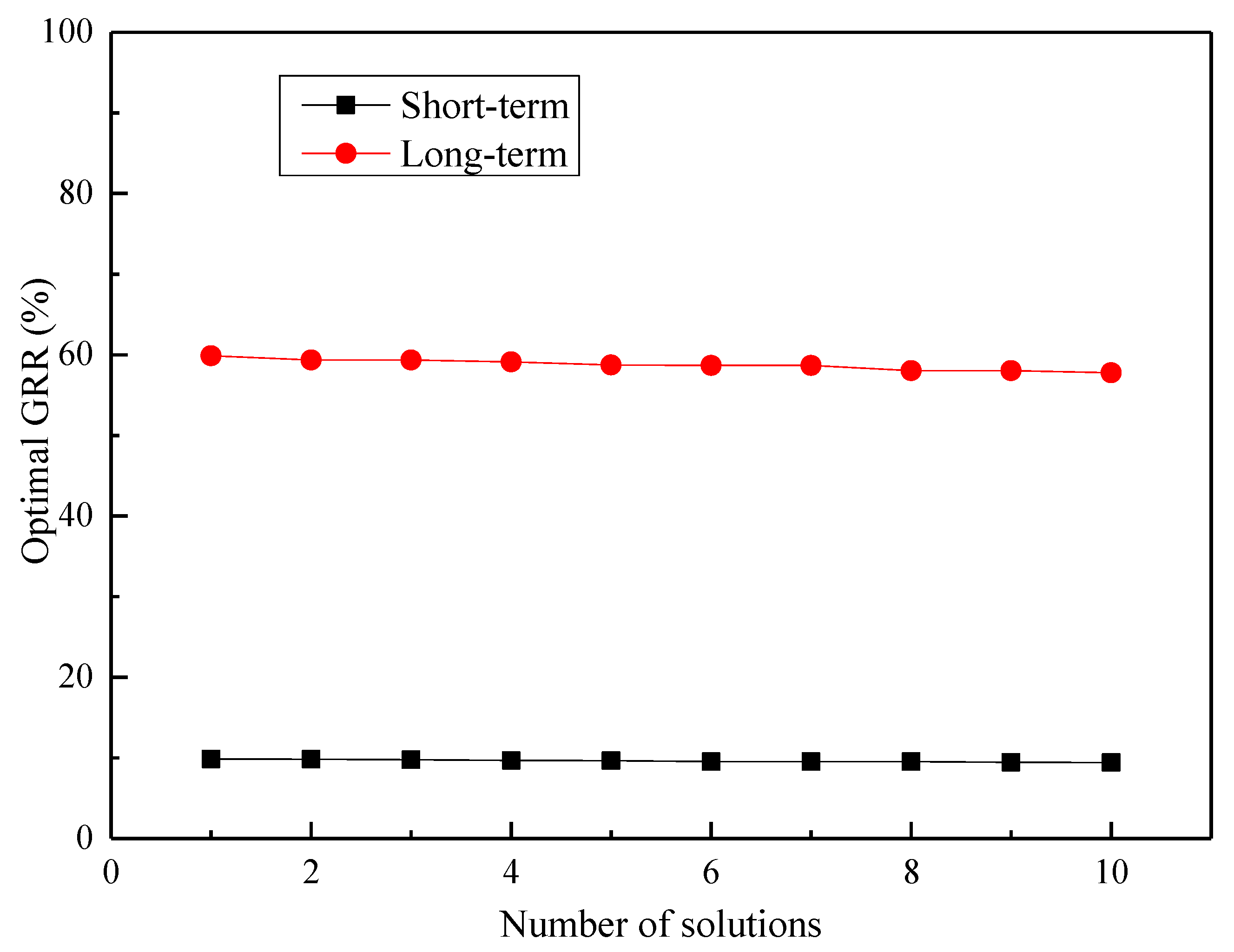
The index of GRR reflects the overall response of the formation subjected to short-term and long-term gas production. Larger index implies more efficient gas production. This index is very important to describe the shale gas productivity. In this study, the numerical optimization with the response surface method is conducted to select the set of variables for the multi-scale gas flow that leads to the maximum GRR. All variables are in their ranges. A total of 100 optimal projects are generated after numerical optimization. Figure 14 and Figure 15 show the top 10 solutions for the maximum GRR and the corresponding responses of GRR. Figure 14 shows that the matrix apparent diffusivity, initial NF aperture, NF density and HF half-length are close to their maximum and have smaller changes for all the desirable solutions. HF spacing locates around the minimum value. NF orientation and initial HF conductivity show higher uncertainty for the 10 solutions. Figure 15 shows the optimal GRRs in the current ranges of parameters are 10% for short-term production and 60% for long-term production. They are in reasonable ranges according to [2]. It is noted that this study did not investigate other parameters such as bottom-hole pressure, in-situ stress, and gas adsorption parameters, although these parameters are very important to gas production [2,39,40]. This optimization process indicated that the optimization room is relatively small, but sensitivity analysis reveals that matrix diffusion plays an incomparable role in gas production. Thus, the optimization results depend on matrix diffusion over other parameters.
5. Conclusions
In this study, the response surface methodology is combined with a fully coupled hydro-mechanical FEC-DPM to explore the influence of seven uncertain factors (i.e., matrix apparent diffusivity, initial NF aperture, NF density, NF orientation, initial HF conductivity, HF half-length and spacing) on the gas recovery rate (GRR) in short-term and long-term productions. An example is numerically analyzed in details. Based on these investigations, the following insights and conclusions can be made.
First, the proposed approach is feasible and efficient for the design and optimization of multi-stage hydraulically fractured horizontal wells with multi-parameters. The GRR response surface model is reliable in the prediction compared with the actual values of GRR. RSM combining with reservoir simulation model can be not only an alternative optimization method, but also a tool for parameter sensitivity analysis.
Second, the influence of these seven uncertain factors for short-term production is ranked as: A-Matrix apparent diffusivity > F-HF half-length > B-Initial NF aperture > E-Initial HF conductivity > G-HF spacing > C-NF density > D-NF orientation. This ranking for long-term production becomes: A-Matrix apparent diffusivity > C-NF density > F-HF half-length > B-Initial NF aperture > E-Initial HF conductivity > G-HF spacing> D-NF orientation. Therefore, the matrix apparent diffusivity plays the most important role in short-term and long-term gas productions although hydraulic fracturing is a vital factor.
Third, optimization results show that the gas recovery rate can reach 10% in short-term and 60% in long-term if the multi-factor optimization of these parameters is done for a multi-stage hydraulically fractured shale gas horizontal well. Therefore, combining hydraulic fracturing with an auxiliary method may be an effective alternative method for the maximum GRR in the development of shale gas.
As a final remark, this study conducted the optimal design solutions by RSM optimization for shale gas production. The visualization of gas recovery rate evolution in the present numerical modeling throws new lights on the understanding of interactions among multi-scale controlling variables. These analyses provide a deep insight into the sensitivity analysis as well as the contributions of different factors on maximizing the gas recovery rate through an optimization model. These analyses also indicate that some artificial treatments, such as heating recovery, can be carried out to improve gas recovery rate. This is a topic for our further study.
Acknowledgments
The authors are grateful to the financial supports from the China Scholarship Council (CSC, Grant No. 201706420033) and the National Natural Science Foundation of China (Grant No. 51674246).
Author Contributions
Jia Liu proposed the optimization model, implemented the numerical simulations and prepared the draft of manuscript. Jianguo Wang designed and modified the theoretical framework and the structures of manuscript; Chunfai Leung corrected English. Feng Gao deduced some equations and revised some Figures.
Conflicts of Interest
The authors declare no conflict of interest.
Nomenclature
| Proppant pack compressibility index, dimensionless | |
| 4th order elasticity tensor which is the inverse of the total elastic compliance tensor, GPa | |
| Gas apparent diffusivity in shale matrix, m2/s | |
| Body force, N/m3 | |
| Shape factor, m−2 | |
| Identity tensor | |
| GRR objective function with key parameters, % | |
| Solid bulk modulus of the grain, GPa | |
| Permeability of hydraulic fractures, m2 | |
| Fracture normal stiffness, GPa/m | |
| Total fracture shear stiffness, GPa/m | |
| , | Shear stiffness before and after shear, respectively, GPa/m |
| Permeability tensor of natural fracture, m2 | |
| Apparent molecular weight of shale gas, kg/mol | |
| Initial reservoir pressure, Pa | |
| Langmuir pressure constant, Pa | |
| Gas pressure at standard condition, Pa | |
| Bottom hole pressure, Pa | |
| Universal gas constant, J·mol−1·K−1 | |
| Reservoirs temperature, K | |
| Displacement vector, m | |
| Vector of the unknown parameters | |
| Optimal combination of the parameters | |
| Reservoir volume, m3 | |
| Langmuir volume (at standard condition), m3/m3 | |
| Fracture width, mm | |
| Z-factor of shale gas, dimensionless | |
| Greek symbols | |
| Porosity for shale matrix, fractures system and hydraulic fracture, fraction | |
| Effective shear dilation angle, rad | |
| Total stress, Pa | |
| Effective stress acting on fracture surface, Pa | |
| Volumetric strain, dimensionless | |
| Density of adsorbed gas | |
| Shale gas density, kg/m3 | |
| Shale gas density at standard condition, kg/m3 | |
| , | Fitting parameters, dimensionless |
| Maximum closure of natural fracture | |
| shear stress of fracture, Pa | |
| shear strength of fracture, Pa | |
| Gas viscosity, Pa·s | |
| Total gas content, kg/m3 | |
| Subscripts | |
| Matrix | |
| Natural fractures | |
| Hydraulic fractures | |
References
- Ambrose, R.J.; Hartman, R.C.; Campos, M.D.; Akkutlu, I.Y.; Sondergeid, C. Shale Gas-in-Place Calculations Part I: New Pore-Scale Considerations. SPE J. 2012, 17, 219–229. [Google Scholar] [CrossRef]
- Yu, W.; Sepehrnoori, K. An efficient reservoir-simulation approach to design and optimize unconventional gas production. J. Can. Pet. Technol. 2014, 53, 109–121. [Google Scholar] [CrossRef]
- Liu, J.; Wang, J.G.; Gao, F.; Ju, Y.; Zhang, X.; Zhang, L. Flow consistency between non-Darcy flow in fracture network and nonlinear diffusion in matrix to gas production rate in fractured shale gas reservoirs. Transp. Porous Media 2016, 111, 97–121. [Google Scholar] [CrossRef]
- Liu, J.; Wang, J.G.; Gao, F.; Ju, Y.; Tang, F. Impact of micro- and macro-consistent flows on well performance in fractured shale gas reservoirs. J. Nat. Gas Sci. Eng. 2016, 36, 1239–1252. [Google Scholar] [CrossRef]
- Zhang, C.; Gamage, R.P.; Perera, M.S.A.; Zhao, J. Characteristics of clay-abundant shale formations: use of CO2 for production enhancement. Energies 2017, 10, 1887. [Google Scholar] [CrossRef]
- Yu, W.; Luo, Z.; Javadpour, F.; Varavei, A.; Sepehrnoori, K. Sensitivity analysis of hydraulic fracture geometry in shale gas reservoirs. J. Pet. Sci. Eng. 2014, 113, 1–7. [Google Scholar] [CrossRef]
- Hyman, J.D.; Jiménezmartínez, J.; Viswanathan, H.S.; Carey, J.W.; Porter, M.L.; Rougier, E.; Karra, S.; Kang, Q.; Frash, L.; Chen, L.; et al. Understanding hydraulic fracturing: A multi-scale problem. Philos. Trans. 2016, 374, 20150426. [Google Scholar] [CrossRef] [PubMed]
- Salama, A.; Amin, M.F.E.; Kumar, K.; Sun, S. Flow and Transport in Tight and Shale Formations: A Review. Geofluids 2017, 2017, 4251209. [Google Scholar] [CrossRef]
- Kim, J.; Kang, J.M.; Park, C.; Park, Y.; Park, J.; Lim, S. Multi-objective history matching with a proxy model for the characterization of production performances at the shale gas reservoir. Energies 2017, 10, 579. [Google Scholar] [CrossRef]
- Zhang, D.; Dai, Y.; Ma, X.; Zhang, L.; Zhong, B.; Wu, J.; Tao, Z. An analysis for the influences of fracture network system on multi-stage fractured horizontal well productivity in shale gas reservoirs. Energies 2018, 11, 414. [Google Scholar] [CrossRef]
- Pan, Z.; Connell, L.D. Reservoir simulation of free and adsorbed gas production from shale. J. Nat. Gas Sci. Eng. 2015, 22, 359–370. [Google Scholar] [CrossRef]
- Gao, F.; Liu, J.; Wang, J.G.; Ju, Y.; Leung, C. Impact of micro-scale heterogeneity on gas diffusivity of organic-rich shale matrix. J. Nat. Gas Sci. Eng. 2017, 45, 75–87. [Google Scholar] [CrossRef]
- Peng, Y.; Liu, J.; Pan, Z.; Connell, L.D. A sequential model of shale gas transport under the influence of fully coupled multiple processes. J. Nat. Gas Sci. Eng. 2015, 27, 808–821. [Google Scholar] [CrossRef]
- Liu, J.; Wang, J.G.; Gao, F.; Leung, C.F.; Ma, Z.G. A fully coupled fracture equivalent continuum-dual porosity model for hydro-mechanical process in fractured shale gas reservoirs. Comput. Geotech. 2017. in review. [Google Scholar]
- Liu, G.R.; Zhou, J.J.; Wang, J.G. Coefficient identification in electronic system cooling simulation through genetic algorithm. Comput. Struct. 2002, 80, 23–30. [Google Scholar] [CrossRef]
- Rahman, M.M.; Sarma, H.K.; Dhabi, A. Maximizing tight gas recovery through a new hydraulic fracture optimization model. In Proceedings of the SPE Reservoir Characterisation and Simulation Conference and Exhibition, Abu Dhabi, UAE, 9–11 October 2011. [Google Scholar]
- Holt, S. Numerical Optimization of Hydraulic Fracture Stage Placement in a Gas Shale Reservoir. Master’s Thesis, TU Deflt University, Deflt, The Netherlands, 2011. [Google Scholar]
- Ma, X.; Plaksina, T.; Gildin, E. Optimization of Placement of Hydraulic Fracture Stages in Horizontal Wells Drilled in Shale Gas Reservoirs. In Proceedings of the Unconventional Resources Technology Conference, Denver, CO, USA, 12–14 August 2013; pp. 1479–1489. [Google Scholar]
- Li, J.C.; Gong, B.; Wang, H.G. Mixed integer simulation optimization for optimal hydraulic fracturing and production of shale gas fields. Eng. Opt. 2016, 48, 1378–1400. [Google Scholar] [CrossRef]
- Rammay, M.H.; Awotunde, A.A. Stochastic optimization of hydraulic fracture and horizontal well parameters in shale gas reservoirs. J. Nat. Gas Sci. Eng. 2016, 36, 71–78. [Google Scholar] [CrossRef]
- Yu, W.; Sepehrnoori, K. Optimization of multiple hydraulically fractured horizontal wells in unconventional gas reservoirs. J. Pet. Eng. 2013, 2013, 151898. [Google Scholar]
- Wang, Y.; Li, X.; Zhang, B.; Zhao, Z. Optimization of multiple hydraulically fractured factors to maximize the stimulated reservoir volume in silty laminated shale formation, Southeastern Ordos Basin, China. J. Pet. Sci. Eng. 2016, 145, 370–381. [Google Scholar] [CrossRef]
- Wang, Y.; Li, X.; Hu, R.; Ma, C.; Zhao, Z.; Zhang, B. Numerical evaluation and optimization of multiple hydraulically fractured parameters using a flow-stress-damage coupled approach. Energies 2016, 9, 325. [Google Scholar] [CrossRef]
- Myers, R.H.; Montgomery, D.C. Response Surface Methodology: Process and Product Optimization Using Designed Experiments; John Wiley and Sons: Hoboken, NJ, USA, 2002. [Google Scholar]
- Kazemi, H.; Gilman, J.R.; Elsharkawy, A.M. Analytical and numerical solution of oil recovery from fractured reservoirs with empirical transfer functions. SPE Reserv. Eng. 1992, 7, 219–227. [Google Scholar] [CrossRef]
- Wen, Q.; Wang, S.; Duan, X.; Li, Y.; Wang, F.; Jin, X. Experimental investigation of proppant settling in complex hydraulic-natural fracture system in shale reservoirs. J. Nat. Gas Sci. Eng. 2016, 33, 70–80. [Google Scholar] [CrossRef]
- Tan, Y.; Pan, Z.; Liu, J.; Wu, Y.; Haque, A.; Connell, L.D. Experimental study of permeability and its anisotropy for shale fracture supported with proppant. J. Nat. Gas Sci. Eng. 2017, 44, 250–264. [Google Scholar] [CrossRef]
- Li, K.; Gao, Y.; Lyu, Y.; Wang, M. New mathematical models for calculating proppant embedment and fracture conductivity. SPE J. 2015, 20, 496–507. [Google Scholar] [CrossRef]
- Li, H.; Wang, K.; Xie, J.; Li, Y.; Zhu, S. A new mathematical model to calculate sand-packed fracture conductivity. J. Nat. Gas Sci. Eng. 2016, 35, 567–582. [Google Scholar] [CrossRef]
- Neto, L.B.; Khanna, A.; Kotousov, A. Conductivity and performance of hydraulic fractures partially filled with compressible proppant packs. Int. J. Rock Mech. Min. Sci. 2015, 74, 1–9. [Google Scholar]
- Guo, J.C.; Lu, C.; Zhao, J.Z. Experimental research on propant embedment. J. China Coal Soc. 2008, 33, 661–664. (In Chinese) [Google Scholar]
- Lu, C.; Guo, J.; Wang, W. Experimental research on proppant embedment and its damage to fractures conductivity. Nat. Gas Ind. 2008, 28, 99–101. [Google Scholar]
- Grieser, B.; Shelley, B.; Soliman, M. Predicting production outcome from multi-stage, horizontal Barnett completions. In Proceedings of the SPE Production and Operations Symposium, Oklahoma City, OK, USA, 4–8 April 2009. Paper SPE 120271. [Google Scholar]
- Garcia-Teijeiro, X.; Rodriguez-Herrera, A.; Fischer, K. The interplay between natural fractures and stress as controls to hydraulic fracture geometry in depleted reservoirs. J. Nat. Gas Sci. Eng. 2016, 34, 318–330. [Google Scholar] [CrossRef]
- Iranmanesh, S.; Mehrali, M.; Sadeghinezhad, E.; Ang, B.C.; Ong, H.C.; Esmaeilzadeh, A. Evaluation of viscosity and thermal conductivity of graphene nanoplatelets nanofluids through a combined experimental–statistical approach using respond surface methodology method. Int. Commun. Heat Mass Transf. 2016, 79, 74–80. [Google Scholar] [CrossRef]
- Kazemi-Beydokhti, A.; Namaghi, H.Z.; Heris, S.Z. Identification of the key variables on thermal conductivity of Cuo nanofluid by a fractional factorial design approach. Numer. Heat Transf. Part B Fundam. 2013, 64, 480–495. [Google Scholar] [CrossRef]
- Teng, T.; Wang, J.G.; Gao, F.; Ju, Y. Complex thermal coal-gas interactions in heat injection enhanced CBM recovery. J. Nat. Gas Sci. Eng. 2016, 34, 1174–1190. [Google Scholar] [CrossRef]
- Kang, Y.L.; Chen, M.J.; Chen, Z.X.; You, L.J.; Hao, Z.W. Investigation of formation heat treatment to enhance the multiscale gas transport ability of shale. J. Nat. Gas Sci. Eng. 2016, 35, 265–275. [Google Scholar] [CrossRef]
- Yu, W.; Sepehrnoori, K. Simulation of gas desorption and geomechanics effects for unconventional gas reservoirs. Fuel 2014, 116, 455–464. [Google Scholar] [CrossRef]
- Yu, W.; Zhang, T.; Du, S.; Sepehrnoori, K. Numerical study of the effect of uneven proppant distribution between multiple fractures on shale gas well performance. Fuel 2015, 142, 189–198. [Google Scholar] [CrossRef]
Figure 1.
Numerical model of multi-stage hydraulically fractured shale reservoir horizontal well.

Figure 2.
Flow chart of framework for RSM optimization of gas production.
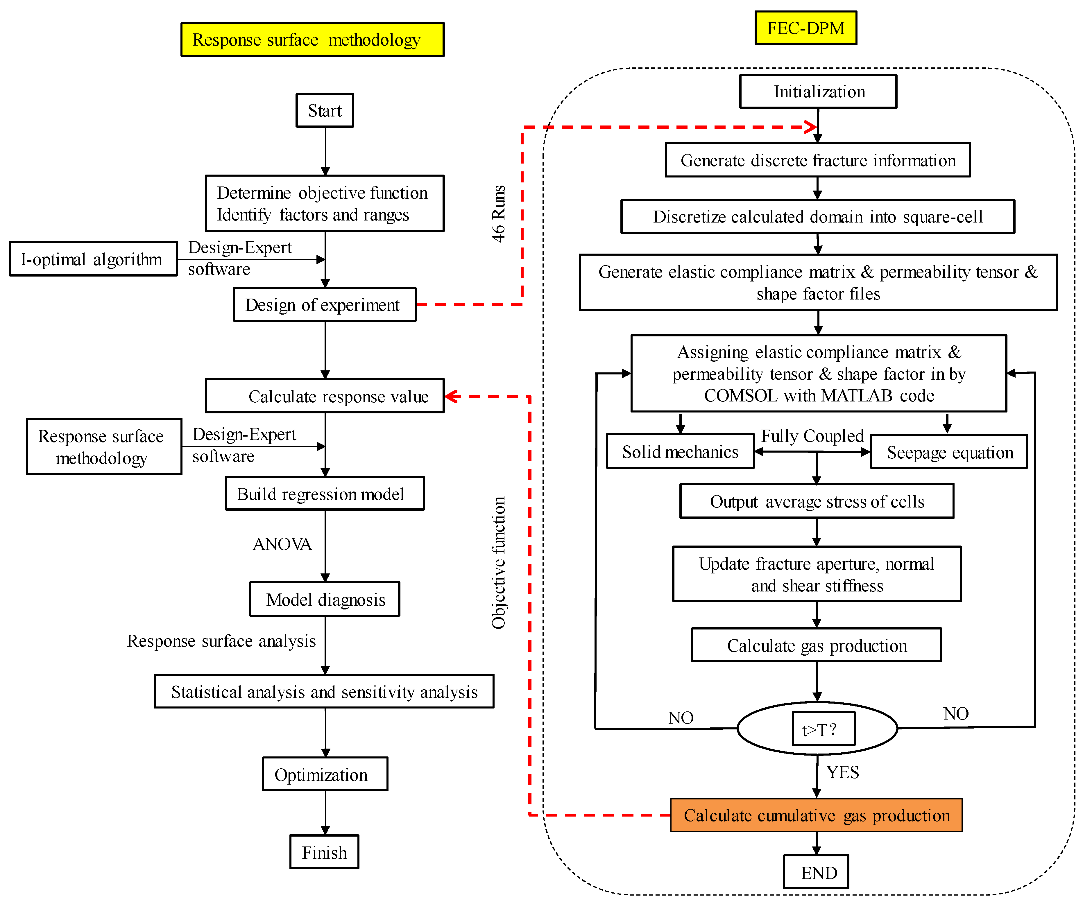
Figure 3.
Fitting for proppant embedment by power law model. (a) Proppant embedment test 1 [31]; (b) Proppant embedment test 2 [32].
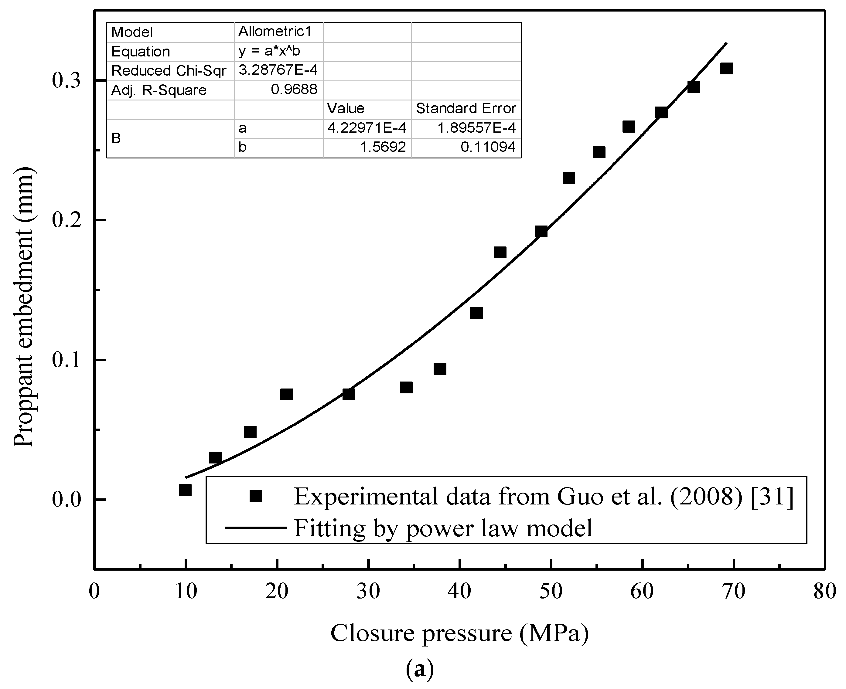
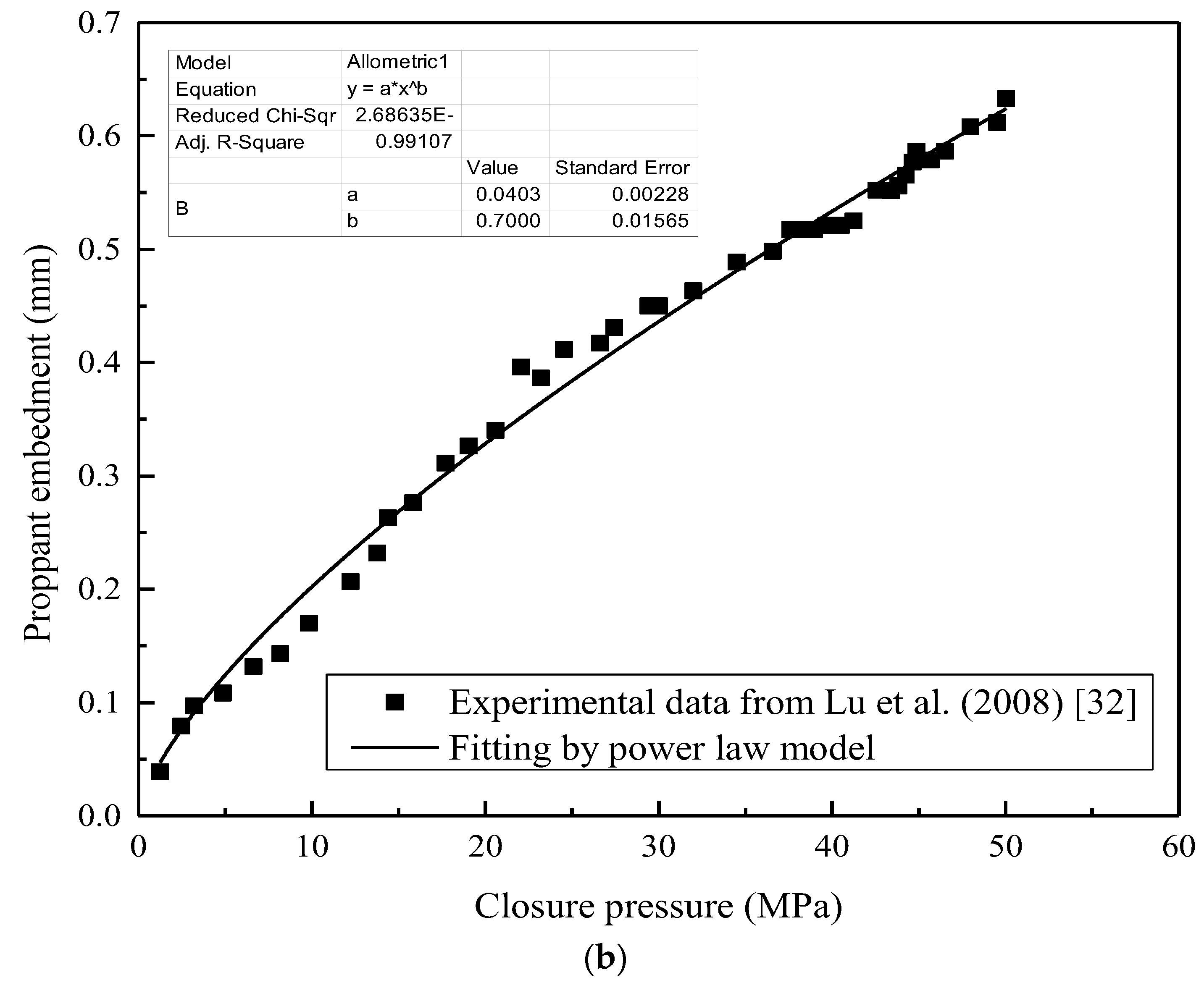
Figure 4.
(a) Numerical model with four hydraulic fractures in the Barnett Shale and (b) history matching for gas production rate and accumulative gas production.
Figure 4.
(a) Numerical model with four hydraulic fractures in the Barnett Shale and (b) history matching for gas production rate and accumulative gas production.
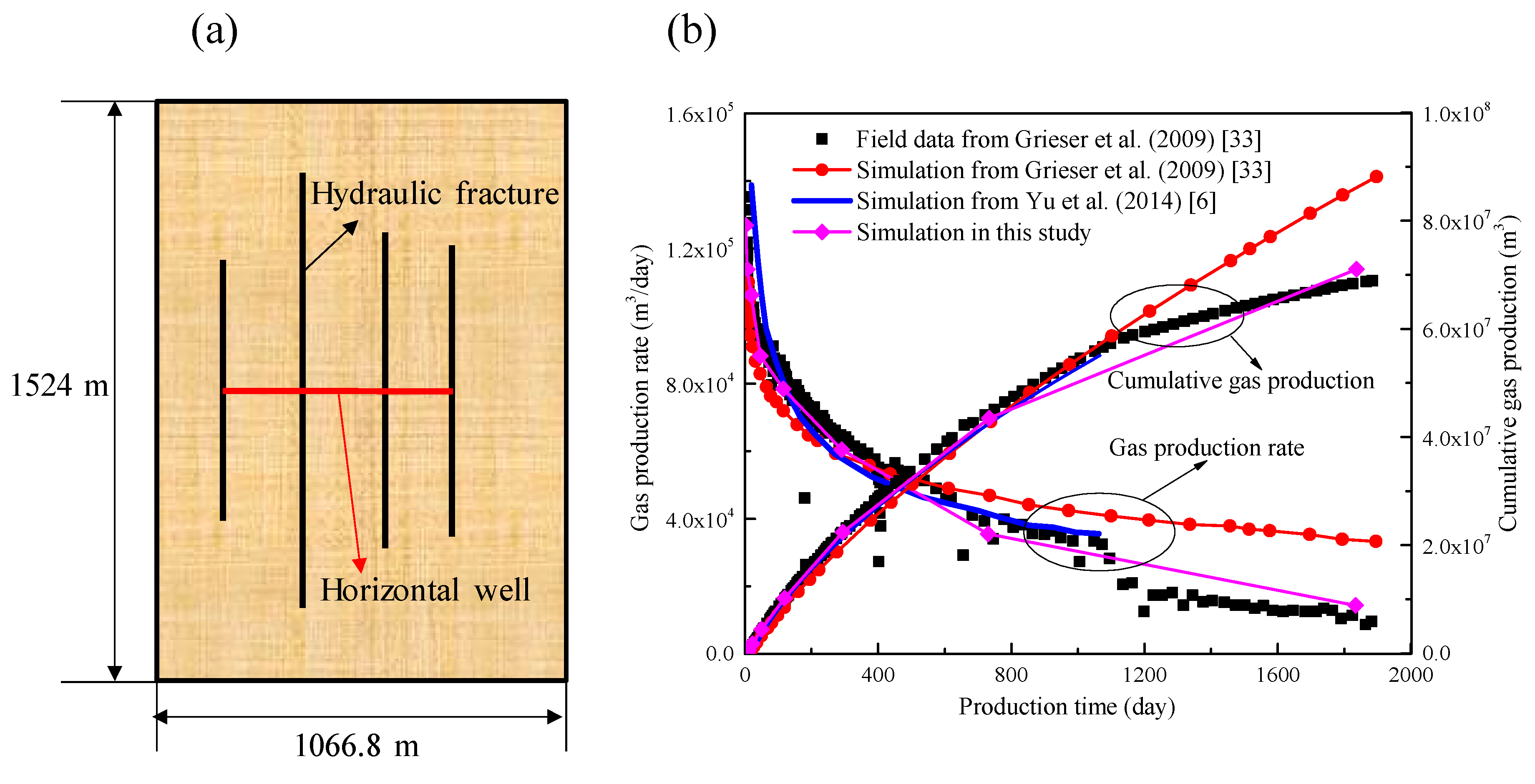
Figure 5.
Gas recovery rates of 46 simulation cases without/with geomechanics.
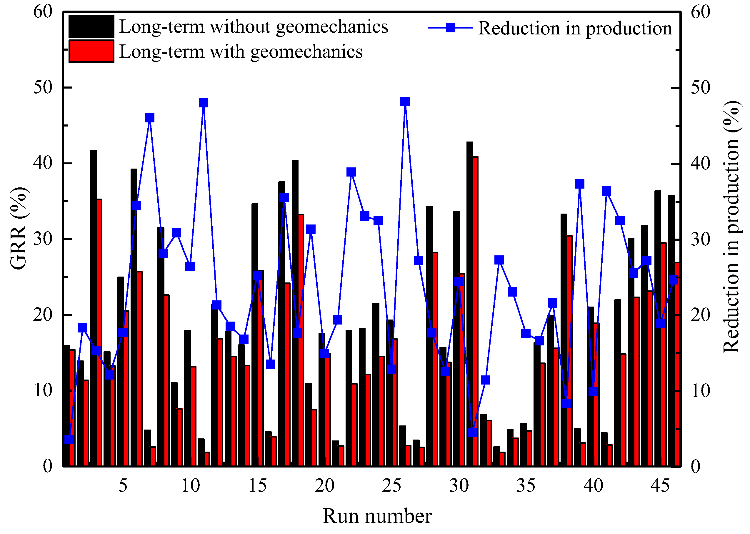
Figure 6.
Histograms of GRRs of 46 runs in short-term and long-term gas productions with geomechanics.
Figure 6.
Histograms of GRRs of 46 runs in short-term and long-term gas productions with geomechanics.
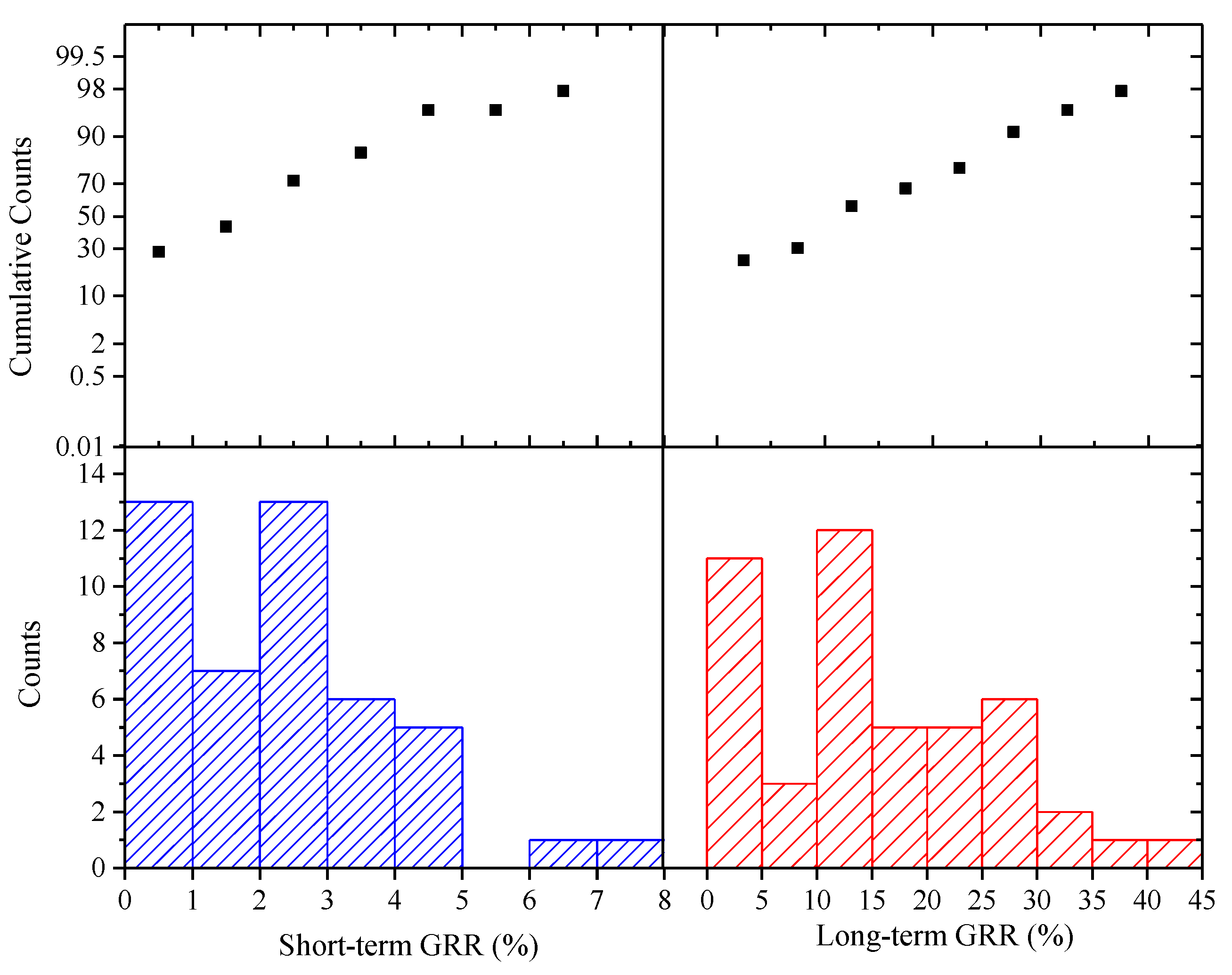
Figure 7.
Gas pressure distribution from simulation results for the partial 4 runs in short-term and long-term gas production according to Table 2.
Figure 7.
Gas pressure distribution from simulation results for the partial 4 runs in short-term and long-term gas production according to Table 2.
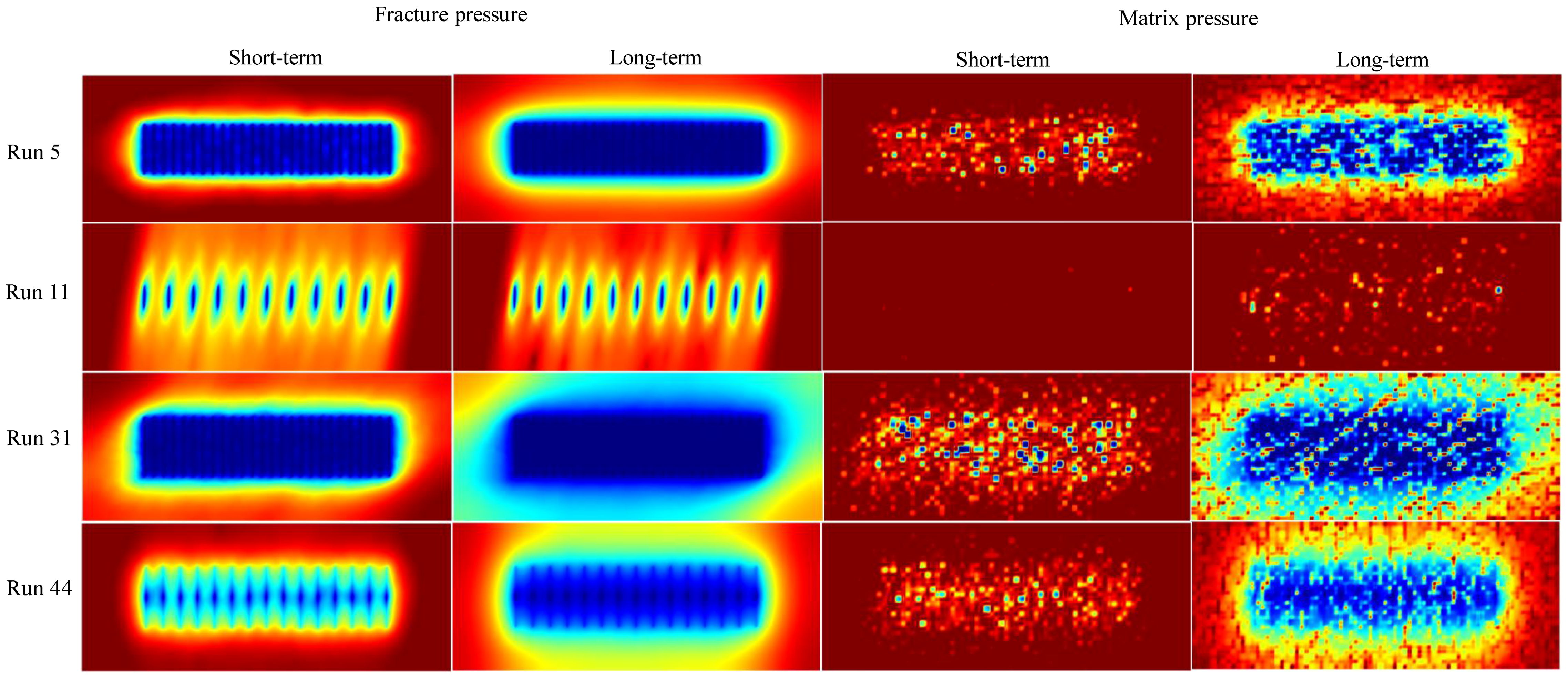
Figure 8.
Normal plot of residuals at different production period.

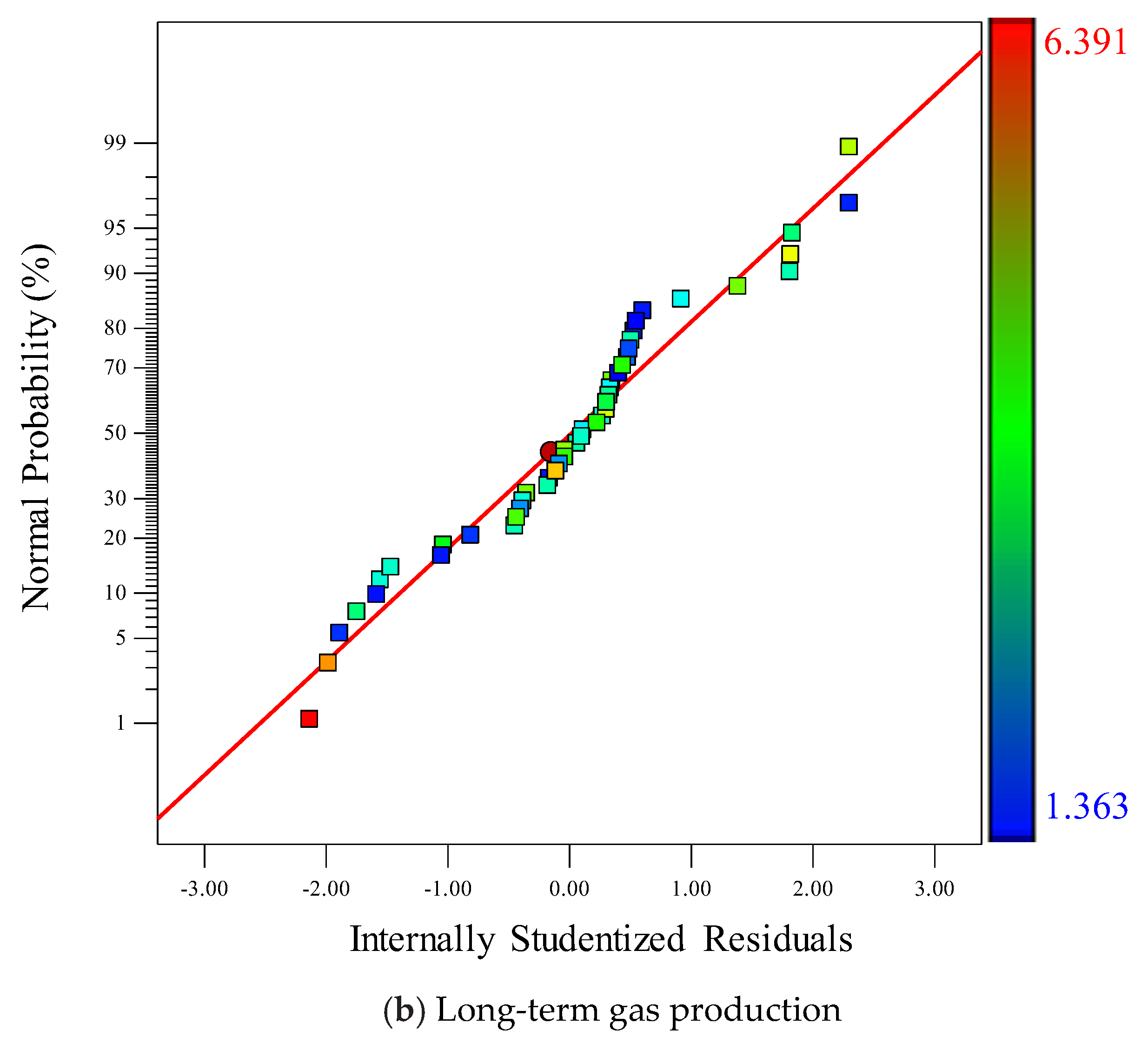
Figure 9.
Predicted versus actual plot at different production periods.
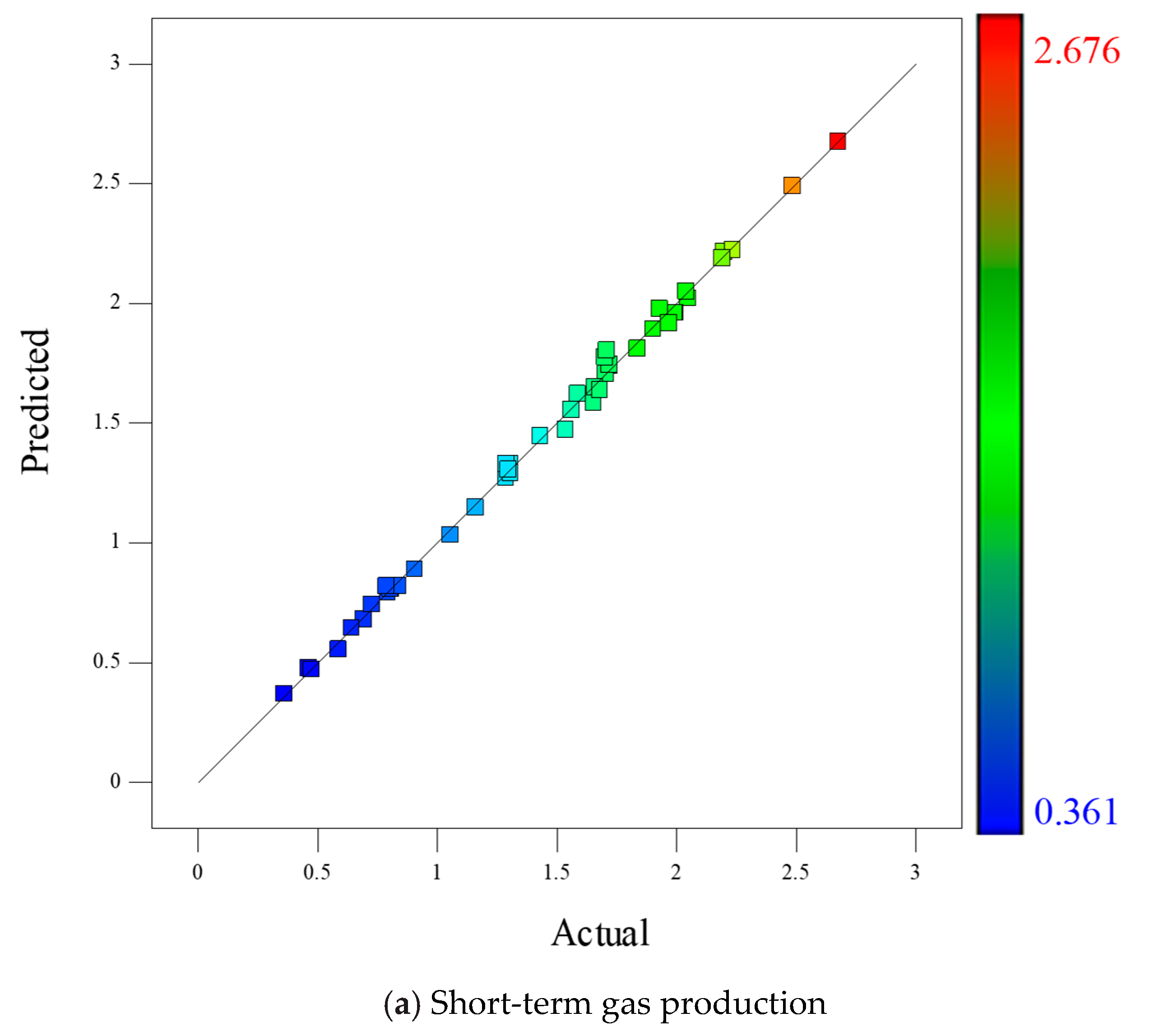
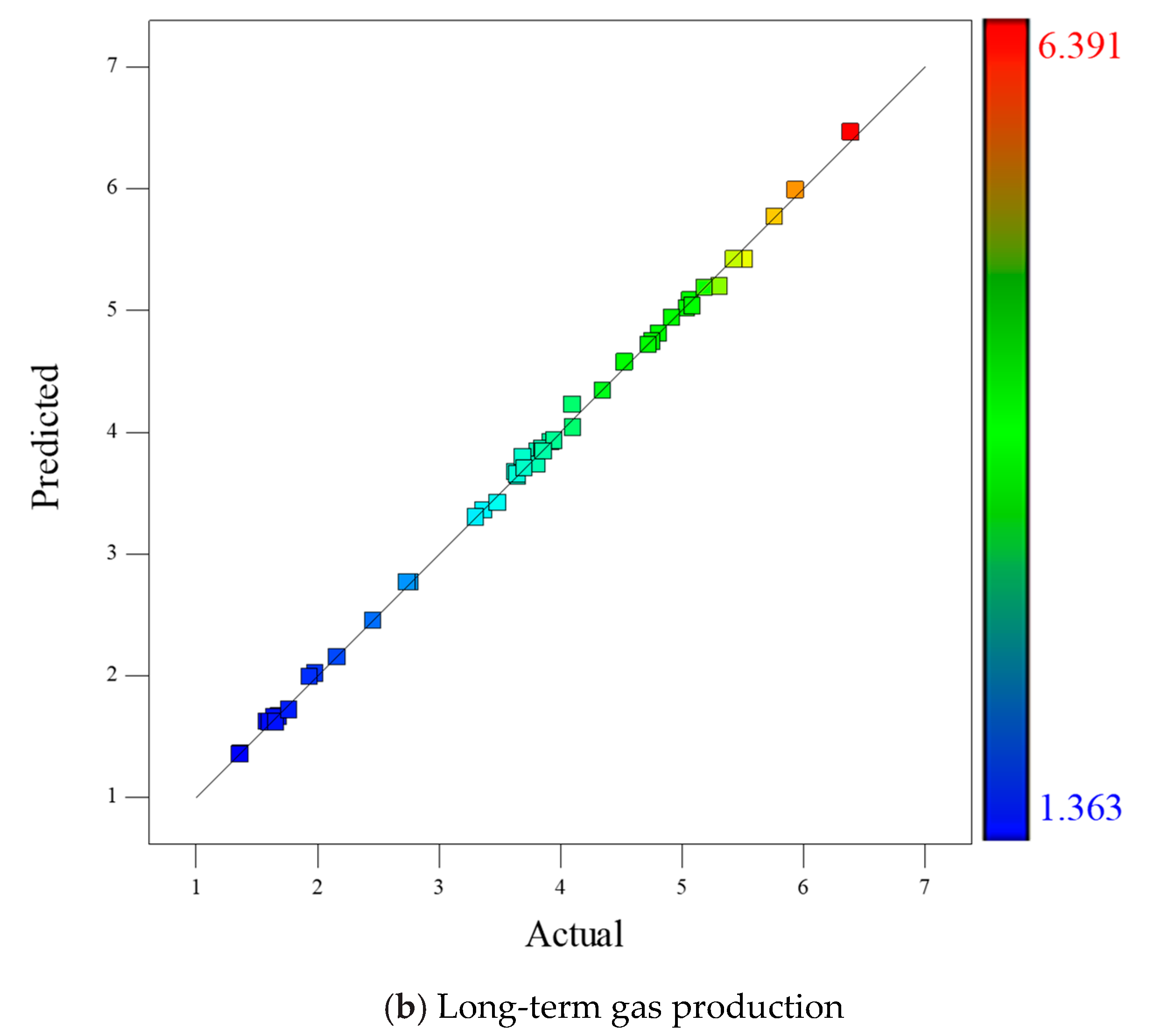
Figure 10.
The Studentized residuals and predicted responses at different production periods.
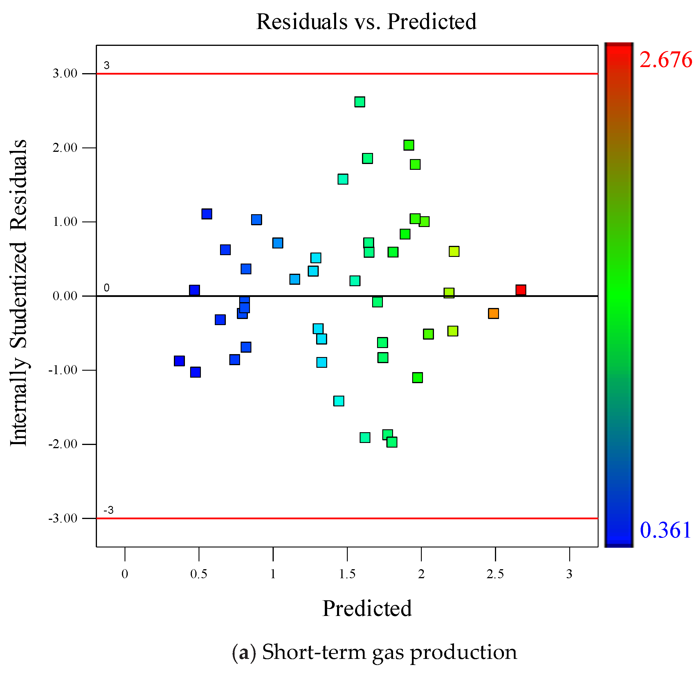

Figure 11.
Studentized residuals versus run number at different production periods.
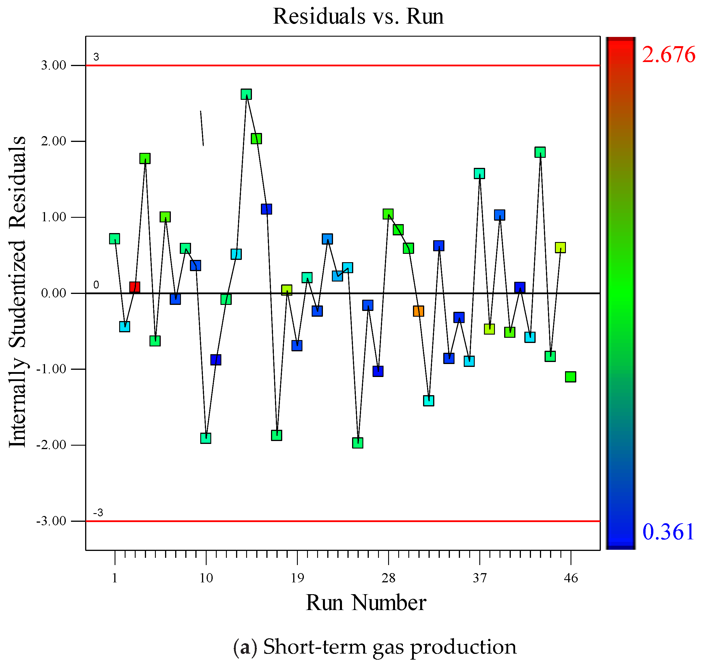
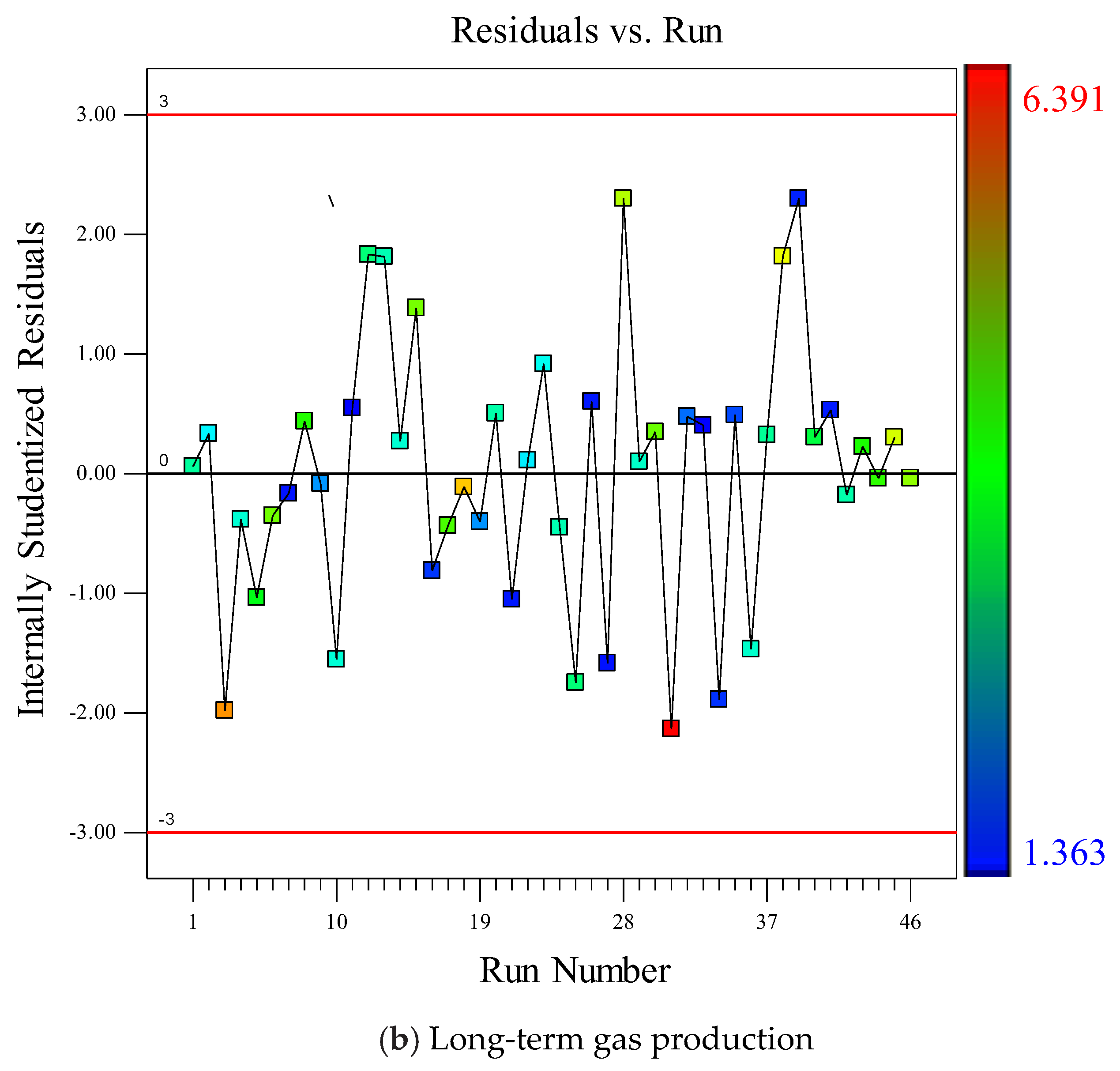
Figure 12.
Influences of factors on GRR for short-term and long-term gas production.
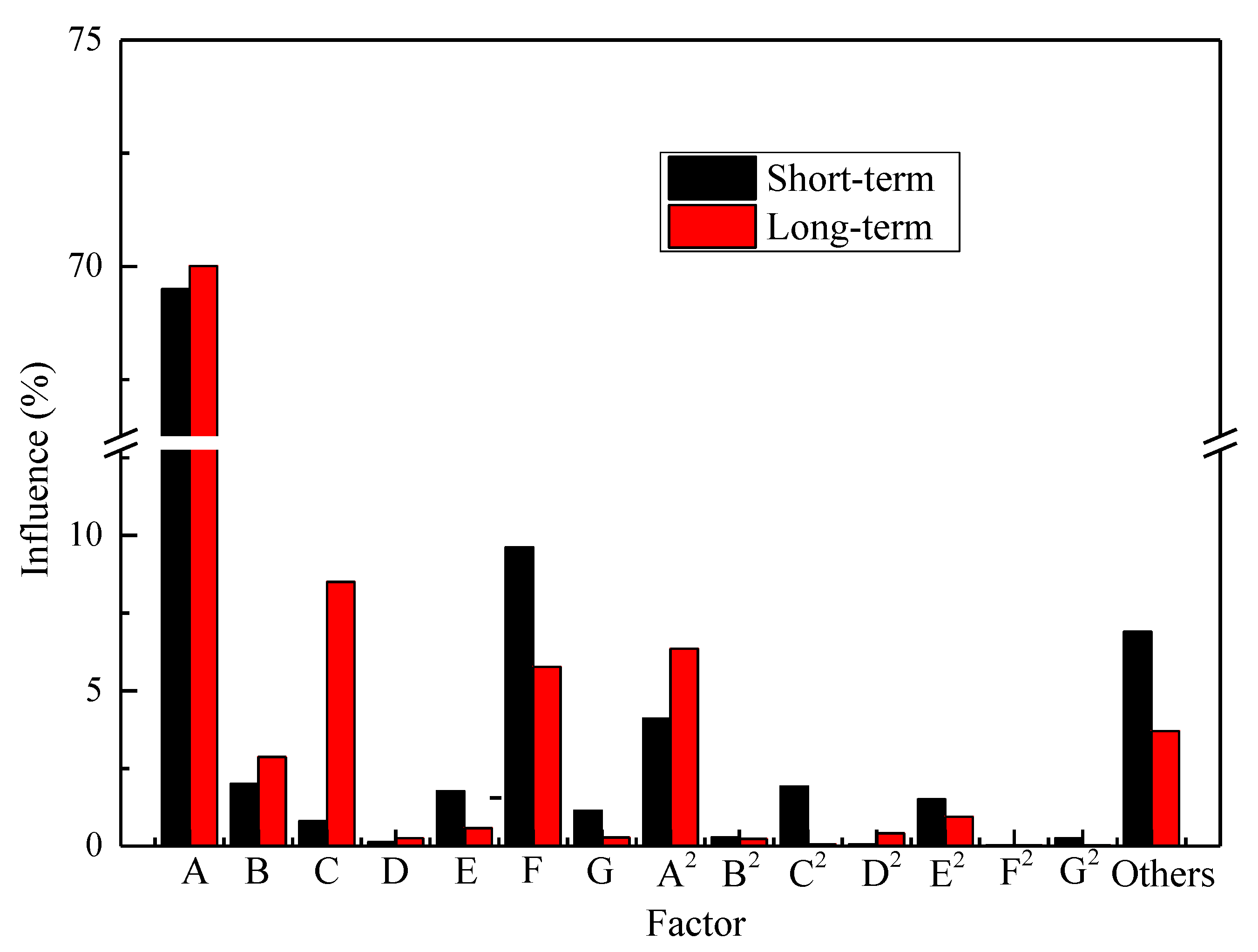
Figure 13.
3D surface for interaction effect of two-parameter on long-term GRR response at fixed values of other parameters ((a) Influence of matrix apparent diffusivity and initial NF aperture on GRR; (b) Influence of initial NF aperture and NF density on GRR; (c) Influence of NF density and NF orientation on GRR; (d) Influence of NF orientation and initial HF conductivity on GRR; (e) Influence of initial HF conductivity and HF half-length on GRR; (f) Influence of HF half-length and HF spacing on GRR).
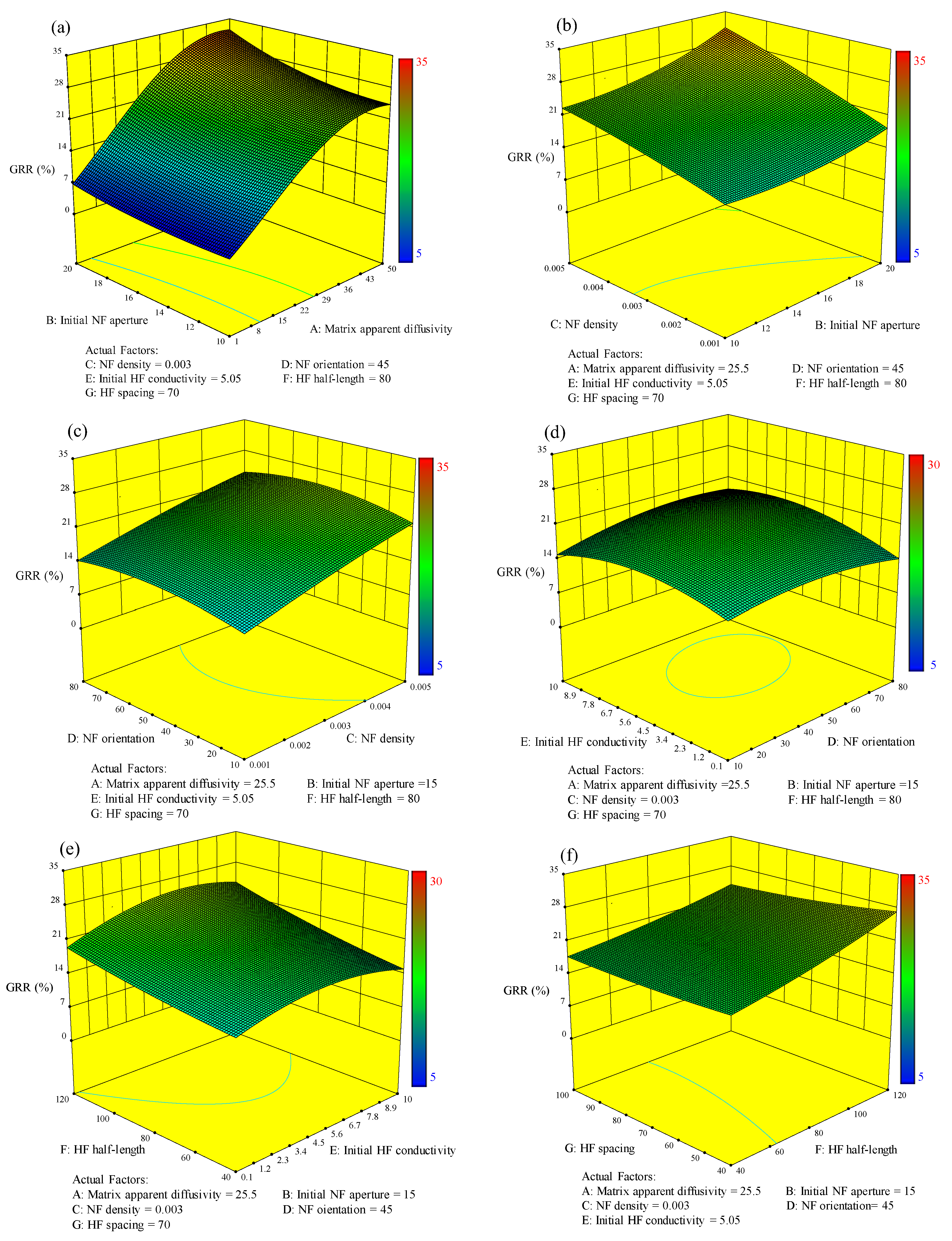
Figure 14.
Magnitudes of variables for the desired top 10 solutions of GRR ((a) Influence of matrix parameter; (b–d) are influence of natural fracture parameters; (e–g) are influence of hydraulic fracture parameters).
Figure 14.
Magnitudes of variables for the desired top 10 solutions of GRR ((a) Influence of matrix parameter; (b–d) are influence of natural fracture parameters; (e–g) are influence of hydraulic fracture parameters).

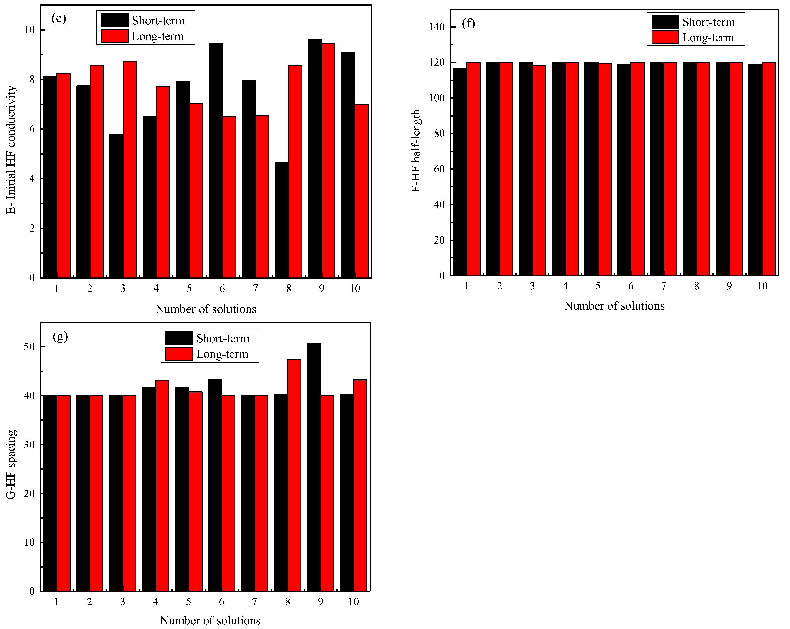
Figure 15.
Optimal GRR for top 10 solutions.

Table 1.
Optimization parameter in this study.
| Parameters | Coded Symbol | Minimum (−1) | Maximum (+1) | Unit |
|---|---|---|---|---|
| Matrix diffusivity | A | 1 | 50 | 10−8 m2/s |
| Initial NF aperture | B | 10 | 20 | µm |
| Density of NF | C | 0.001 | 0.005 | fraction |
| Orientation of NF | D | 10 | 80 | degree |
| Initial HF conductivity | E | 0.1 | 10 | µm2·cm |
| HF half-length | F | 40 | 120 | m |
| HF spacing | G | 40 | 100 | m |
Table 2.
I-optimal design table.
| Run | A | B | C | D | E | F | G |
|---|---|---|---|---|---|---|---|
| 1 | 50.00 | 10.00 | 0.001 | 10.00 | 2.38 | 40 | 40 |
| 2 | 42.65 | 10.00 | 0.001 | 80.00 | 0.10 | 40 | 100 |
| 3 | 50.00 | 10.00 | 0.005 | 80.00 | 10.00 | 120 | 40 |
| 4 | 19.87 | 10.00 | 0.001 | 80.00 | 5.20 | 120 | 40 |
| 5 | 17.42 | 10.00 | 0.005 | 10.00 | 3.86 | 100 | 40 |
| 6 | 50.00 | 17.00 | 0.005 | 42.20 | 0.10 | 40 | 40 |
| 7 | 1.00 | 15.08 | 0.001 | 50.60 | 6.04 | 40 | 70 |
| 8 | 16.93 | 20.00 | 0.004 | 56.20 | 10.00 | 80 | 100 |
| 9 | 2.23 | 12.65 | 0.004 | 47.80 | 8.52 | 120 | 70 |
| 10 | 28.56 | 20.00 | 0.001 | 80.00 | 0.10 | 40 | 40 |
| 11 | 1.00 | 10.00 | 0.005 | 80.00 | 10.00 | 40 | 100 |
| 12 | 50.00 | 16.90 | 0.001 | 56.55 | 0.10 | 100 | 70 |
| 13 | 28.20 | 20.00 | 0.002 | 10.00 | 0.64 | 60 | 70 |
| 14 | 27.71 | 14.75 | 0.001 | 33.80 | 10.00 | 80 | 40 |
| 15 | 50.00 | 10.00 | 0.004 | 49.55 | 5.10 | 80 | 100 |
| 16 | 1.00 | 20.00 | 0.005 | 80.00 | 0.10 | 40 | 70 |
| 17 | 44.12 | 20.00 | 0.005 | 55.15 | 0.10 | 40 | 100 |
| 18 | 50.00 | 20.00 | 0.005 | 80.00 | 0.25 | 120 | 100 |
| 19 | 2.23 | 12.65 | 0.004 | 47.80 | 8.52 | 120 | 70 |
| 20 | 50.00 | 20.00 | 0.001 | 10.00 | 10.00 | 40 | 100 |
| 21 | 1.00 | 16.35 | 0.002 | 13.50 | 0.10 | 120 | 40 |
| 22 | 15.70 | 13.40 | 0.004 | 17.00 | 2.08 | 40 | 100 |
| 23 | 15.70 | 13.40 | 0.004 | 17.00 | 2.08 | 40 | 40 |
| 24 | 30.79 | 10.00 | 0.003 | 43.95 | 10.00 | 40 | 70 |
| 25 | 48.53 | 14.02 | 0.001 | 24.35 | 5.57 | 80 | 100 |
| 26 | 1.00 | 15.08 | 0.001 | 50.6 | 6.04 | 40 | 70 |
| 27 | 1.00 | 19.70 | 0.004 | 10.00 | 10.00 | 40 | 40 |
| 28 | 17.17 | 18.10 | 0.005 | 74.05 | 5.20 | 100 | 40 |
| 29 | 20.36 | 18.90 | 0.001 | 10.00 | 6.49 | 120 | 100 |
| 30 | 48.78 | 16.75 | 0.003 | 80.00 | 6.83 | 60 | 70 |
| 31 | 50.00 | 20.00 | 0.003 | 29.25 | 5.99 | 120 | 40 |
| 32 | 1.00 | 20.00 | 0.001 | 80.00 | 10.00 | 120 | 40 |
| 33 | 1.00 | 10.00 | 0.002 | 10.00 | 10.00 | 80 | 100 |
| 34 | 2.23 | 16.70 | 0.002 | 80.00 | 1.83 | 100 | 100 |
| 35 | 1.00 | 20.00 | 0.005 | 10.00 | 0.10 | 120 | 100 |
| 36 | 25.34 | 11.00 | 0.002 | 10.00 | 0.30 | 80 | 70 |
| 37 | 50.00 | 20.00 | 0.001 | 80.00 | 0.84 | 40 | 100 |
| 38 | 50.00 | 10.00 | 0.003 | 10.00 | 9.26 | 120 | 40 |
| 39 | 1.00 | 10.00 | 0.001 | 25.40 | 0.10 | 120 | 100 |
| 40 | 44.12 | 12.53 | 0.001 | 80.00 | 10.00 | 120 | 100 |
| 41 | 1.00 | 10.00 | 0.004 | 73.00 | 0.10 | 60 | 40 |
| 42 | 30.79 | 10.00 | 0.003 | 43.95 | 10.00 | 40 | 40 |
| 43 | 50.00 | 13.50 | 0.003 | 10.00 | 0.10 | 120 | 100 |
| 44 | 32.85 | 10.50 | 0.005 | 80.00 | 0.10 | 120 | 70 |
| 45 | 46.08 | 16.80 | 0.005 | 10.00 | 10.00 | 80 | 70 |
| 46 | 48.78 | 16.75 | 0.003 | 80.00 | 6.83 | 60 | 40 |
Table 3.
Computational parameters used in simulations.
| Parameters | Value |
|---|---|
| Model size, m | 1500 × 600 × 100 |
| Elastic modulus, E (GPa) | 20.68 |
| Solid bulk modulus, ks (GPa) | 37.82 |
| Poisson’s ratio, ν | 0.25 |
| Bulk density, ρ (kg/m3) | 2400 |
| Maximum horizontal stress, (MPa) | 43.34 |
| Minimum horizontal stress, (MPa) | 39.01 |
| Initial reservoir pressure, pi (MPa) | 28.27 |
| Bottom hole pressure, pw (MPa) | 15 |
| Biot coefficient, αB | 0.64 |
| Fracture shear stiffness, (GPa/M) | 434 |
| Initial normal stiffness, Kn0 (GPa/M) | 434 |
| Friction angle, (°) | 24.9 |
| Dilation angle, (°) | 5 |
| Methane dynamic viscosity, μ (Pa·s) | 2.01 × 10⁻⁵ |
| Reservoir temperature, T (K) | 350 |
| Langmuir pressure constant, PL (MPa) | 10 |
| Langmuir volume constant, VL (m3/m3) | 10 |
| Density of adsorbed gas in the organic pores, ρads (kg/m3) | 370 |
| Matrix porosity φm | 0.04 |
| Hydraulic fracture porosity φF | 0.3 |
Table 4.
(a) Statistics approach to select the RSM model for short-term production. (b) Statistics approach to select the RSM model for long-term production.
Table 4.
(a) Statistics approach to select the RSM model for short-term production. (b) Statistics approach to select the RSM model for long-term production.
| Source | Std. Dev. | R-Squared | Adjusted R-Squared | Predicted R-Squared | PRESS | Fit or Not | |
|---|---|---|---|---|---|---|---|
| (a) | |||||||
| Linear | 0.25 | 0.8495 | 0.8218 | 0.7799 | 3.38 | - | |
| 2FI | 0.26 | 0.9265 | 0.8054 | −0.0031 | 15.40 | - | |
| Quadratic | 0.065 | 0.9972 | 0.9874 | 0.8706 | 1.99 | Suggested | |
| Cubic | 0.025 | 0.9999 | 0.9982 | - | - | Aliased | |
| (b) | |||||||
| Linear | 0.51 | 0.8862 | 0.8653 | 0.8296 | 14.96 | - | |
| 2FI | 0.63 | 0.9235 | 0.7975 | −0.3208 | 115.93 | - | |
| Quadratic | 0.097 | 0.9989 | 0.9952 | 0.9485 | 4.52 | Suggested | |
| Cubic | 0.029 | 1.0000 | 0.9996 | - | - | Aliased | |
Table 5.
(a) ANOVA for GRR in short-term response surface with quadratic model. (b) ANOVA for GRR in long-term response surface with quadratic model.
Table 5.
(a) ANOVA for GRR in short-term response surface with quadratic model. (b) ANOVA for GRR in long-term response surface with quadratic model.
| Source | Sum of Squares | df | Mean Square | F Value | p-Value Prob > F | Significant or Not |
|---|---|---|---|---|---|---|
| (a) | ||||||
| Model | 15.31 | 35 | 0.44 | 101.97 | <0.0001 | significant |
| A | 8.85 | 1 | 8.85 | 2061.94 | <0.0001 | - |
| B | 0.26 | 1 | 0.26 | 59.46 | <0.0001 | - |
| C | 0.10 | 1 | 0.10 | 23.76 | 0.0006 | - |
| D | 0.016 | 1 | 0.016 | 3.73 | 0.0823 | - |
| E | 0.23 | 1 | 0.23 | 52.56 | <0.0001 | - |
| F | 1.22 | 1 | 1.22 | 285.53 | <0.0001 | - |
| G | 0.14 | 1 | 0.14 | 33.69 | 0.0002 | - |
| AB | 3.759 × 10⁻³ | 1 | 3.759 × 10⁻³ | 0.88 | 0.3713 | - |
| AC | 0.43 | 1 | 0.43 | 99.09 | <0.0001 | - |
| AD | 2.101 × 10⁻³ | 1 | 2.101 × 10⁻³ | 0.49 | 0.5000 | - |
| AE | 8.553 × 10⁻³ | 1 | 8.553 × 10⁻³ | 1.99 | 0.1883 | - |
| AF | 0.071 | 1 | 0.071 | 16.62 | 0.0022 | - |
| AG | 0.017 | 1 | 0.017 | 4.06 | 0.0714 | - |
| BC | 0.019 | 1 | 0.019 | 4.47 | 0.0607 | - |
| BD | 0.061 | 1 | 0.061 | 14.33 | 0.0036 | - |
| BE | 0.038 | 1 | 0.038 | 8.85 | 0.0139 | - |
| BF | 3.217 × 10⁻³ | 1 | 3.217 × 10⁻³ | 0.75 | 0.4068 | - |
| BG | 5.927 × 10⁻³ | 1 | 5.927 × 10⁻³ | 1.38 | 0.2670 | - |
| CD | 0.011 | 1 | 0.011 | 2.53 | 0.1430 | - |
| CE | 0.021 | 1 | 0.021 | 4.96 | 0.0500 | - |
| CF | 4.226 × 10⁻³ | 1 | 4.226 × 10⁻³ | 0.99 | 0.3443 | - |
| CG | 0.015 | 1 | 0.015 | 3.42 | 0.0943 | - |
| DE | 6.599 × 10⁻³ | 1 | 6.599 × 10⁻³ | 1.54 | 0.2432 | - |
| DF | 1.172 × 10⁻⁶ | 1 | 1.172 × 10⁻⁶ | 2.733×10⁻⁴ | 0.9871 | - |
| DG | 0.030 | 1 | 0.030 | 6.98 | 0.0247 | - |
| EF | 0.028 | 1 | 0.028 | 6.62 | 0.0278 | - |
| EG | 0.081 | 1 | 0.081 | 18.85 | 0.0015 | - |
| FG | 0.025 | 1 | 0.025 | 5.94 | 0.0350 | - |
| A2 | 0.52 | 1 | 0.52 | 121.85 | <0.0001 | - |
| B2 | 0.036 | 1 | 0.036 | 8.37 | 0.0160 | - |
| C2 | 0.24 | 1 | 0.24 | 56.93 | <0.0001 | - |
| D2 | 6.635 × 10⁻³ | 1 | 6.635 × 10⁻³ | 1.55 | 0.2420 | - |
| E2 | 0.19 | 1 | 0.19 | 44.65 | <0.0001 | - |
| F2 | 2.860 × 10⁻³ | 1 | 2.860 × 10⁻³ | 0.67 | 0.4333 | - |
| G2 | 0.032 | 1 | 0.032 | 7.46 | 0.0211 | - |
| Residual | 0.043 | 10 | 4.290 × 10⁻³ | - | ||
| Lack of Fit | 0.042 | 8 | 5.207 × 10⁻³ | 8.36 | 0.1112 | not significant |
| Pure Error | 1.246 × 10⁻³ | 2 | 6.230 × 10⁻⁴ | - | ||
| Cor Total | 15.35 | 45 | - | |||
| (b) | ||||||
| Model | 87.68 | 35 | 2.51 | 267.44 | <0.0001 | significant |
| A | 53.13 | 1 | 53.13 | 5672.42 | <0.0001 | - |
| B | 2.18 | 1 | 2.18 | 232.70 | <0.0001 | - |
| C | 6.45 | 1 | 6.45 | 689.12 | <0.0001 | - |
| D | 0.19 | 1 | 0.19 | 20.42 | 0.0011 | - |
| E | 0.44 | 1 | 0.44 | 46.94 | <0.0001 | - |
| F | 4.37 | 1 | 4.37 | 466.98 | <0.0001 | - |
| G | 0.21 | 1 | 0.21 | 22.32 | 0.0008 | - |
| AB | 0.048 | 1 | 0.048 | 5.08 | 0.0478 | - |
| AC | 0.36 | 1 | 0.36 | 38.06 | 0.0001 | - |
| AD | 0.035 | 1 | 0.035 | 3.76 | 0.0810 | - |
| AE | 0.035 | 1 | 0.035 | 3.75 | 0.0816 | - |
| AF | 0.21 | 1 | 0.21 | 22.53 | 0.0008 | - |
| AG | 0.099 | 1 | 0.099 | 10.55 | 0.0088 | - |
| BC | 0.14 | 1 | 0.14 | 15.11 | 0.0030 | - |
| BD | 0.57 | 1 | 0.57 | 61.09 | <0.0001 | - |
| BE | 0.44 | 1 | 0.44 | 46.61 | <0.0001 | - |
| BF | 5.167 × 10⁻⁵ | 1 | 5.167 × 10⁻⁵ | 5.516 × 10⁻³ | 0.9423 | - |
| BG | 1.154 × 10⁻⁴ | 1 | 1.154 × 10⁻⁴ | 0.012 | 0.9138 | - |
| CD | 9.434 × 10⁻³ | 1 | 9.434 × 10⁻³ | 1.01 | 0.3392 | - |
| CE | 0.028 | 1 | 0.028 | 3.03 | 0.1126 | - |
| CF | 0.25 | 1 | 0.25 | 26.87 | 0.0004 | - |
| CG | 0.13 | 1 | 0.13 | 13.88 | 0.0039 | - |
| DE | 0.22 | 1 | 0.22 | 23.34 | 0.0007 | - |
| DF | 2.136 × 10⁻³ | 1 | 2.136 × 10⁻³ | 0.23 | 0.6432 | - |
| DG | 1.290 × 10⁻³ | 1 | 1.290 × 10⁻³ | 0.14 | 0.7183 | - |
| EF | 0.092 | 1 | 0.092 | 9.78 | 0.0107 | - |
| EG | 0.049 | 1 | 0.049 | 5.27 | 0.0446 | - |
| FG | 0.095 | 1 | 0.095 | 10.14 | 0.0098 | - |
| A2 | 4.82 | 1 | 4.82 | 514.41 | <0.0001 | - |
| B2 | 0.17 | 1 | 0.17 | 18.27 | 0.0016 | - |
| C2 | 0.049 | 1 | 0.049 | 5.20 | 0.0457 | - |
| D2 | 0.31 | 1 | 0.31 | 32.94 | 0.0002 | - |
| E2 | 0.72 | 1 | 0.72 | 76.44 | <0.0001 | - |
| F2 | 0.015 | 1 | 0.015 | 1.64 | 0.2290 | - |
| G2 | 0.018 | 1 | 0.018 | 1.90 | 0.1984 | - |
| Residual | 0.094 | 10 | 9.367 × 10⁻³ | - | ||
| Lack of Fit | 0.092 | 8 | 0.012 | 13.86 | 0.0690 | not significant |
| Pure Error | 1.660 × 10⁻³ | 2 | 8.300 × 10⁻⁴ | - | ||
| Cor Total | 87.77 | 45 | - | |||
© 2018 by the authors. Licensee MDPI, Basel, Switzerland. This article is an open access article distributed under the terms and conditions of the Creative Commons Attribution (CC BY) license (http://creativecommons.org/licenses/by/4.0/).
Share and Cite
MDPI and ACS Style
Liu, J.; Wang, J.; Leung, C.; Gao, F. A Multi-Parameter Optimization Model for the Evaluation of Shale Gas Recovery Enhancement. Energies 2018, 11, 654. https://doi.org/10.3390/en11030654
AMA Style
Liu J, Wang J, Leung C, Gao F. A Multi-Parameter Optimization Model for the Evaluation of Shale Gas Recovery Enhancement. Energies. 2018; 11(3):654. https://doi.org/10.3390/en11030654
Chicago/Turabian StyleLiu, Jia, Jianguo Wang, Chunfai Leung, and Feng Gao. 2018. "A Multi-Parameter Optimization Model for the Evaluation of Shale Gas Recovery Enhancement" Energies 11, no. 3: 654. https://doi.org/10.3390/en11030654
Note that from the first issue of 2016, this journal uses article numbers instead of page numbers. See further details here.