A New Analytical Wake Model for Yawed Wind Turbines


Department of Civil Engineering, School of Engineering, The University of Tokyo, 7-3-1 Hongo, Bunkyo-ku, Tokyo 113-8656, Japan
*
Author to whom correspondence should be addressed.
Energies 2018, 11(3), 665; https://doi.org/10.3390/en11030665
Submission received: 26 January 2018
/
Revised: 28 February 2018
/
Accepted: 13 March 2018
/
Published: 15 March 2018
(This article belongs to the Collection Wind Turbines)
Abstract
:A new analytical wake model for wind turbines, considering ambient turbulence intensity, thrust coefficient and yaw angle effects, is proposed from numerical and analytical studies. First, eight simulations by the Reynolds Stress Model are conducted for different thrust coefficients, yaw angles and ambient turbulence intensities. The wake deflection, mean velocity and turbulence intensity in the wakes are systematically investigated. A new wake deflection model is then proposed to analytically predict the wake center trajectory in the yawed condition. Finally, the effects of yaw angle are incorporated in the Gaussian-based wake model. The wake deflection, velocity deficit and added turbulence intensity in the wake predicted by the proposed model show good agreement with the numerical results. The model parameters are determined as the function of ambient turbulence intensity and thrust coefficient, which enables the model to have good applicability under various conditions.
1. Introduction
In an attempt to address the power losses induced by the wake for downstream wind turbines, there have been extensive studies considering adjusting tip speed ratios, blade pitch controls and varying yaw angle [1,2,3]. Yaw control is one of the promising methods for wind farm power optimization, and it is implemented by an intentional yaw misalignment of the turbine to the wind direction [4,5]. This approach relies on an induction of a lateral momentum by actively yawing the upwind turbine to deflect the wake away from the downwind turbines, so that the latter can extract more energy from unwaked flow. Optimization procedures are necessary to maximize the power production of the whole wind farm since there is also a power reduction for the yawed turbine itself. Therefore, accurate evaluations of the deflected wake trajectory and the wake characteristics of a yawed wind turbine are essential for applying yaw control strategies in actual wind farms.
Prediction of the wake characteristics under various yawed conditions requires a detailed understanding of the behavior of wake flow and its interaction with the atmospheric boundary layer. Parkin et al. [6] obtained the detailed velocity field from one to five rotor diameters downstream of a two-bladed wind turbine model under various yaw angles by using PIV and showed the initial skew angle of wakes. Medici and Alfredsson [7] and later Howland et al. [8] performed the hot-wire measurement for a two-bladed and a porous disk model turbine, respectively, and quantified the velocity deficit and deflections in various yawed conditions. Note that these wind tunnel tests were carried out in a uniform flow. Recently, Bastankhah and Porté-Agel [9] systematically studied the wake of a yawed turbine under various thrust coefficients and yaw angles by the detailed wind tunnel measurements in a neutral stratified boundary layer. However, the effects of thrust coefficients and ambient turbulence have not been investigated systematically. Computational fluid dynamics (CFD) has also been widely used to study wind turbine wake flows and power production optimization in a wind farm [10]. Jiménez et al. [11] used large-eddy simulation (LES) to characterize the wake deflections under a range of yaw angles and thrust coefficients for a turbine modeled with a uniformly distributed actuator disk model without rotation (ADM-NR). Later, Fleming et al. [12] applied LES with actuator line model (ALM) to investigate several methods for improving wind plant overall performance, and the yaw control proved to be effective with wake-redirection. Luo et al. [13] conducted the single turbine skew analysis by using LES and showed that the wake deflection was almost linear in the near wake region for moderate yaw angles.
In comparison to wind tunnel tests and numerical simulations, analytical wake models have greater advantages of application in real wind farm because of its simplicity and high efficiency [14]. The wake model for non-yawed turbines and the application in wind farm have been extensively studied [15,16]. By contrast, the analytical studies for the wake under a yawed condition have not received much attention. Jiménez et al. [11] presented a preliminary analysis of wakes on the leeward of a yawed turbine for the first time. He proposed a simple formula to predict the wake skew angle based on the momentum conservation and top-hat model suggested by Jensen [17] for the velocity deficit. However, experimental validation was not sufficient as the author mentioned. Gebraad et al. [5] and Howland et al. [8] derived the formula of yaw induced wake center trajectory by integrating the skew angle proposed by Jiménez et al. [11]. However, the model of Jiménez et al. [11] overestimates the wake deflection since the assumption of top-hat for the velocity deficit is not accurate as pointed out by Ishihara et al. [18]. Based on the theoretical analysis of the governing equations, Bastankhah and Porté-Agel [9] developed an analytical model to predict the wake deflection and the far wake velocity distributions for the yawed turbines. The model showed a good agreement with the experimental data. However, some parameters in this model have not been specified. In addition, the turbulence characteristic in the wake of the yawed turbine is also of great importance as it has a significant impact on the wake development. The investigation of turbulence characteristic and the corresponding analytical model are not included in existing studies.
In this study, a new analytical wake model for a yawed turbine, considering the ambient turbulence intensity, thrust coefficient, and yaw misalignment effects, is proposed. In Section 2, the numerical model and setup used in this study are described. In Section 3, first, the numerical model is validated by comparing with the LES results and then, the wake deflections, mean velocity and turbulence intensity characteristics are systematically investigated. In Section 4, a new analytical wake model for a yawed wind turbine with Gaussian distribution for the velocity deficit and added turbulence intensity is proposed. The accuracy of the proposed model is examined by numerical simulation results for different ambient turbulence intensities, thrust coefficient effects, and yaw angles. Finally, conclusions of this study are summarized in Section 5.
2. Numerical Model
In this section, governing equations and the Reynolds Stress Model (RSM) are introduced firstly. Then, the wind turbine model and the parameters used in the numerical simulations are described.
2.1. Governing Equations
The Reynolds Averaged Navier-Stokes (RANS) equations are used to simulate the turbulent wake flows. The averaged continuity and momentum equations for incompressible flow with external forces can be written in tensor notation and in the Cartesian coordinates as follows
where and are the mean wind velocity in the th direction and the pressure respectively. is density of the fluid and is the molecular viscosity, is the fluid force per unit grid volume induced by the wind turbine. is known as Reynolds stress tensor considering difference between and and it stands for the effect from vortex with the higher frequency in time to the mean flow field which is relatively steady.
2.2. The Turbulence Model
The Reynolds Stress model (RSM) accounts for the anisotropic turbulence stresses to give accurate predictions for complex flows, which is an important advantage compared to the common one-equation and two-equation models with isotropic eddy-viscosity hypothesis. Additionally, as pointed out by Cabezón et al. [19], the common two-equation RANS model like the standard - model could not provide good prediction for the wind turbine wakes, while RSM shows better performance. Some of the modified two-equation model may improve the accuracy but they are still very dependent on how their parameters are tuned for different case.
In this study, the RSM with Linear Pressure-Strain model in ANSYS (Ansys, Inc., Canonsburg, PA, USA) Fluent [20] is used to express the Reynolds stress tensor to close the momentum equation. In RSM, a set of Reynolds stress equations for the turbulence closure are introduced as follows:
where is a model constant with the value of 0.82 according to Lien and Leschziner [21]. is the turbulence viscosity and calculated in the same way as in the - model by using the following equation:
where .
is the term for stress production calculated as
is the pressure strain term, modelled according to the proposals by Gibson and Launder [22], Fu et al. [23], and Launder [24,25], as shown in the following equation
where the model constants and are 1.8 and 0.6, respectively. is the convective term in Equation (3) and calculated by
is the dissipation term modelled as
Equation (3) is solved for each of the different Reynolds stresses. Similar to - model, additional equations are necessary to calculate turbulent kinetic energy and its dissipation rate :
where , , .
Finite volume method is employed, and the simulations are performed with ANSYS Fluent. The default values recommended by the Fluent Theory Guide [20] are used for all the model parameters. The second order upwind scheme is applied for the interpolation of velocities, and Reynolds Stress. SIMPLE (semi-implicit pressure linked equations) algorithm is employed for solving the discretized equations [26].
2.3. Wind Turbine Model
A utility-scale wind turbine model is adopted to study the wake in various yawed conditions. It is based on the offshore 2.4 MW wind turbine at the Choshi demonstration site with the rotor diameter of and hub height of [27]. The effect of the rotor induced forces on the flow is parameterized by using an actuator disk model with rotation (ADM-R), in which the lift and drag forces are calculated based on the blade element theory [28] and then unevenly distributed on the actuator disk. Figure 1 shows the schematic of ADM-R model in a yawed condition, where is streamwise direction aligned with the incoming wind speed and is normal to the rotor plane. The yaw angle denotes the angle between incoming velocity and the rotor normal axial direction . The azimuthal angle shows the position of the blade in the tangential direction and it is 0 at the top position. and are defined positive using the right-hand rule. For the yawed rotor, the velocities and forces need some coordinate transformation when the ADM-R model is applied. The relation between wind velocity and forces acting on a blade element of length located at the radius is shown in Figure 2, where and denote the axial and tangential directions respectively, is the angle of attack, is the local pitch angle and is the angle between the relative velocity and the rotor plane. and are the lift and drag forces acting on the blade element and given by:
where is the chord length, and are the lift and drag coefficients, respectively. is the local relative velocity with respect to the blade element and is defined as:
where and are the axial and tangential velocities of the incident flow at the local blade element position. The resulting axial force and tangential force on the blade element can be expressed as:
The force per unit volume in each annular with an area of and a thickness of is expressed by:
where B is the number of blades.
Based on the Glauert’s [29] moment theory for a yawed rotor, only the normal wind flow component is assumed to be affected by the presence of the rotor and the flow component is left unperturbed by the rotor. The blade element momentum (BEM) theory is still used for the yawed rotor by including the induced velocity nonuniformity correction [28,30]. The axial and tangential components of the incident flow velocity at blades are assumed as and , where is the turbine rotational speed, and are the induction factors in the axial and tangential directions, respectively. The induction factors are unknown and solved based on the axial and angular momentum conservations.
In the wind farm simulation, the free upstream wind speed for a turbine in the farm is not known. Thus, the axial and tangential velocity at the rotor disk and are selected as the unknown parameters instead of and [31,32,33]. In this study, a coupled approach is adopted for the ADM-R model in the yawed condition, in which and are directly obtained from the CFD simulation result of local velocities on the rotor disk by using the following transformation:
The axial and tangential forces are calculated by using the above local velocities on the rotor disk and then distributed through the following transformation.
where, is the source term in Equation (2) for each direction to present the effects of the turbine rotor on the momentum. The rotor can be rotated around the z axis enabling the yaw angle configuration. The nacelle and tower are modeled as a porous media with the packing density of 99.9%.
2.4. Numerical Setup
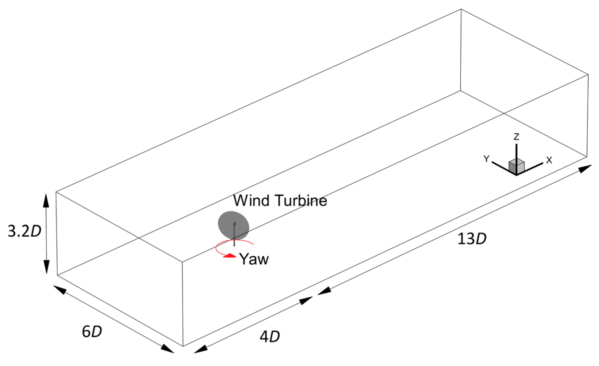
As shown in Figure 3, the computational domain has the streamwise length of 17D, the spanwise length of 6D and the height of 3.2D. The wind turbine model shown in Figure 3 is placed at the center in the spanwise direction, with the rotor diameter D of 0.57 m and the hub height H of 0.7 m. The rotor disk, nacelle and tower are divided in a uniform distance of 0.01 m and then connected smoothly with the main domain by tetrahedral mesh. The main domain is divided by a set of rectangular cells with minimum grid size of 0.001 m near the wall in vertical direction and 0.03 m in horizontal direction. Boundary conditions used in the numerical simulations are summarized in Table 1. The values of extracted at the location of D from the LES simulations conducted by Qian and Ishihara [27] are imposed at the inlet boundary for low and high turbulence boundary layers, respectively. Assuming local equilibrium of production and dissipation of turbulence kinetic energy in streamwise direction, and are given by:
The wall-stress boundary condition is imposed at the ground surface and the roughness height of is used.
Eight simulations are performed to study the effects of three parameters, i.e., the yaw angle , the trust coefficient and the ambient turbulence intensity . The parameters used in the numerical simulations for each case are summarized in Table 2. The thrust coefficient is defined as:
where is the area of rotor, is the thrust force acting on the rotor and is the mean velocity at the hub height. = 0.36 and 0.84 are selected to consider the two kind of operation condition of maximum power and rated power. Two representative yaw angles of 8° and 16° are chosen to consider the maximum yaw misalignment (8) defined by IEC standard [34] and the optimal yaw control angle (10°~30°) based on Gebraad et al. [5].
3. Numerical Results and Discussions
The numerical models used in this study are validated in Section 3.1. Then, the characteristics of the mean velocity and turbulence intensity in the wake region with the different yaw angles are investigated in Section 3.2.
3.1. Validation of Numerical Model
The neutral atmospheric boundary layer profiles without wind turbines are generated by using the inflow condition described in Section 2.4. All the profiles of mean velocity in this study are normalized by the mean wind speed at the hub height. The turbulence intensity is defined as:
where is the normal Reynolds stress in the streamwise direction. Note that the ambient turbulence intensity is the streamwise turbulence intensity upwind the turbine at the hub height. Figure 4 shows the vertical profiles of mean velocity and turbulence intensity at the several streamwise locations, in which dashed lines denote the LES result by Qian and Ishihara [27], solid lines are the RSM results and experimental profiles at the position of turbine () by Ishihara et al. [18] are also plotted together by the open circles. The quantitative comparison by using the Normalized Root Mean Square Error (NRMSE) [35] for each case are summarized in Table 3, in which the mean values of experimental data are used for the normalization. The RSM result shows good agreement with the LES results and the experimental data.
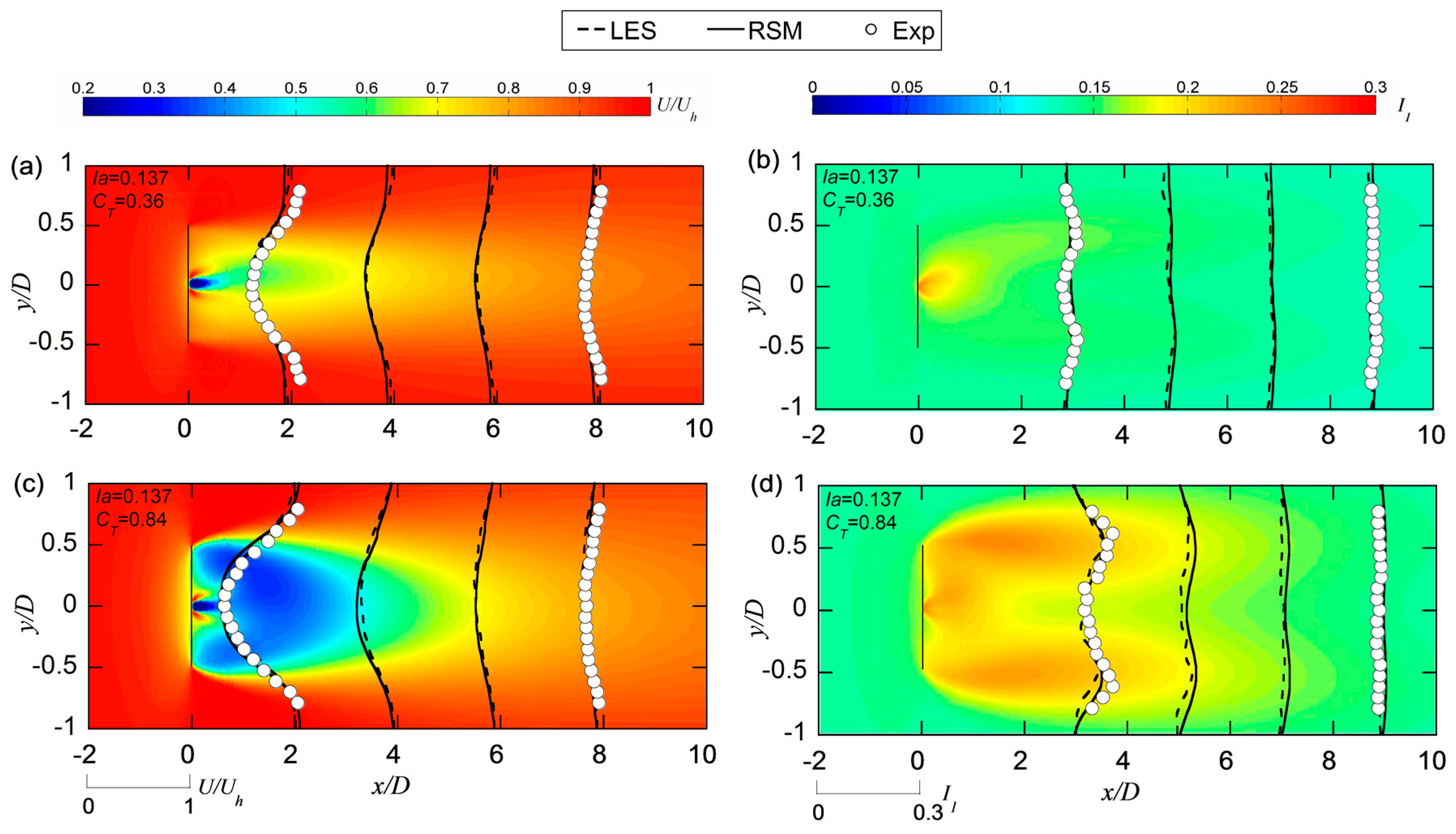
The LES results for the wind turbine wake simulation have been validated with high accuracy by comparison with the experimental data [27]. In order to examine the accuracy of the RSM for wind turbine wake simulation, the mean velocity and turbulence intensity in the wake region under the non-yawed condition are compared with the LES results [27] and experimental data [18] as shown in Figure 5, in which the presented results in contour plots are from RSM. The quantitative comparison by using the NRMSE for each case are summarized in Table 3. The predicted horizontal profiles of mean velocity and turbulence intensity at selected downwind locations by the RSM agree well with the experimental data and show almost same accuracy with LES.
3.2. Mean Velocity and Turbulence Intensity under Yawed Conditions
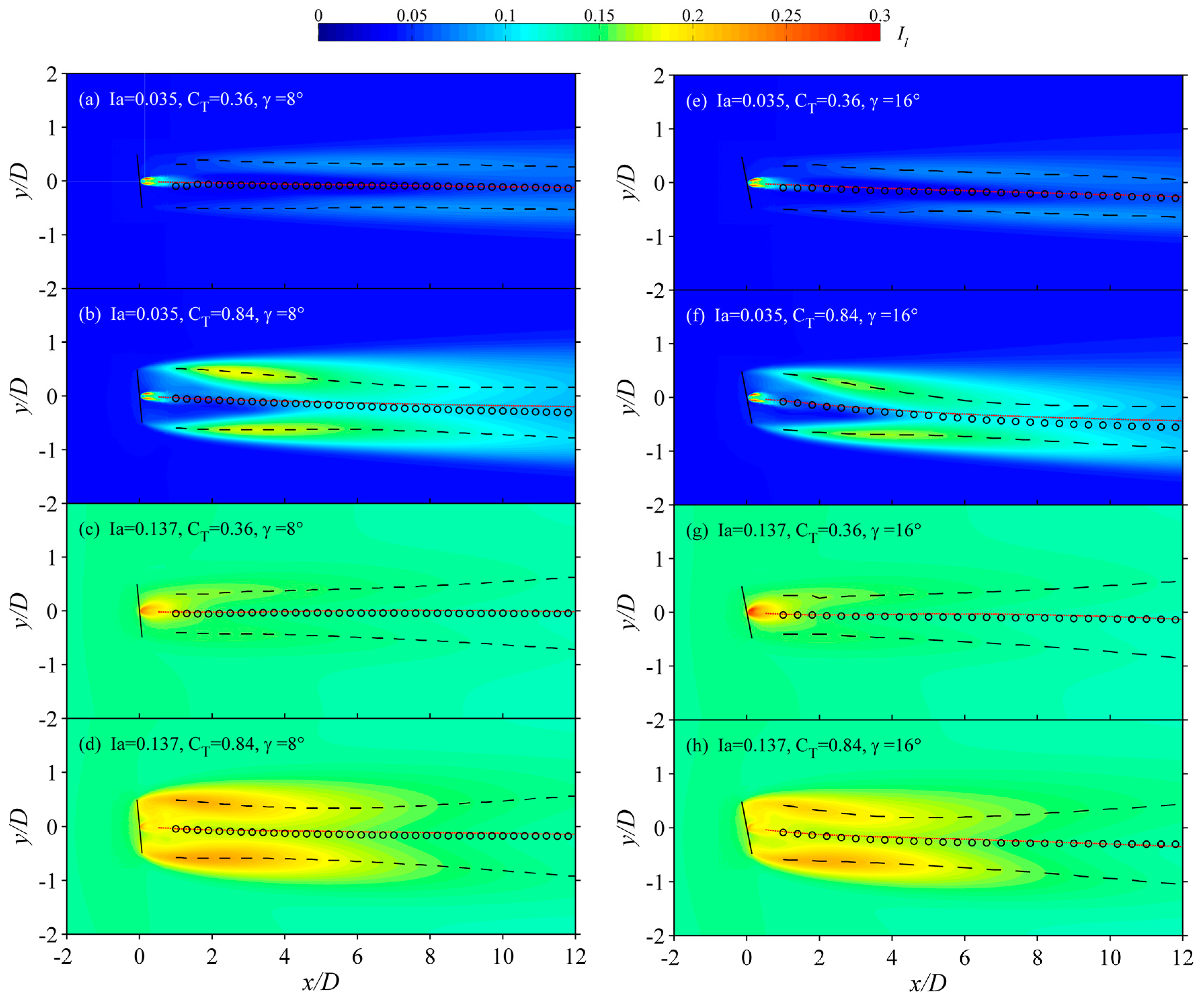
The simulated mean velocity and turbulence intensity by RSM in the wake region under different yawed conditions are shown in Figure 6 and Figure 7. The contours of mean velocity and turbulence intensity as well as wake deflections are displayed in the horizontal - plane at the hub height (). In Figure 6, black dashed lines represent the wake boundary denoted by the positions with the mean wind speed equal to the 95% of the free-stream velocity and the open circles denote the wake centers, which are calculated by taking the midpoint between the wake boundaries, based on the same procedure as Jimenez et al. [11] and Parkin et al. [6]. The black dashed lines in Figure 7 denote the peak values of turbulence intensity at each location and the open circles show the midpoint position of the two peaks.
From Figure 6, it is noticed that the wake velocity deficit reduces when the yaw angle increases. This is consistent with Equation (21) since larger yaw angle induces smaller thrust force on the rotor. In addition, the wake center trajectories show apparent wake deflections under yawed conditions. As expected, the wake deflection increases with the increase of yaw angle. It can also be seen that the large thrust coefficient (Case 2, 4, 6, 8) induces stronger wake deflection than the cases with small thrust coefficient (Case 1, 3, 5, 7). The high ambient turbulence intensity (Case 3, 4, 7, 8) leads to smaller wake deflection and shorter wake region than cases with the low ambient turbulence (Case 1, 2, 5, 6) as the cases under the non-yawed condition. The high turbulence accelerates the process of flow mixing in the wake region, thus both wake deflection and velocity deficit recover faster than those with the low ambient turbulence intensity.
Figure 7 shows that the turbulence intensities in the horizontal x-y plane at the hub height has dual-peak distribution. The wake center trajectories obtained from the mean velocity contours are also plotted together by red dotted lines for comparison. It is found that the midpoint trajectories of turbulence intensity peak trends towards the wake center trajectories. This implies that the turbulence in the wake region are also deflected almost towards the same path as the mean velocity.
4. Analytical Model
A new analytical wake model to predict the wake deflection is derived and validated in Section 4.1. The wake model under non-yawed conditions proposed by Qian and Ishihara [27] is extended by incorporating the yaw angle effects in Section 4.2. Mean velocity and turbulence intensity predicted by the proposed model are compared with those obtained from the numerical simulations.
4.1. A New Analytical Model for the Wake Deflection
As mentioned by Jimenez et al. [11], the wake defection can be explained based on the concept of momentum conservation. When the wind turbine axis is not aligned with the wind direction, the rotor induced thrust forces would add lateral component to the incoming airflow. This lateral force induces a lateral velocity which then causes the wake to deflect towards one side. Jimenez et al. [11] proposed an analytical model to evaluate the wake deflection based on this concept and the assumption of top-hat for the velocity deficit and the skew angle of the wake deflection as shown in Appendix A. However, this model overestimates the wake deflection since the assumption of the top-hat for the velocity deficit is not accurate as pointed out by Ishihara et al. [18]. Recently, Bastankhah and Porté-Agel [9] proposed an analytical model based on the assumption of the Gaussian distribution for the velocity deficit and the skew angle of the wake deflection as described in Appendix B, However, the parameters in this model were not specified.
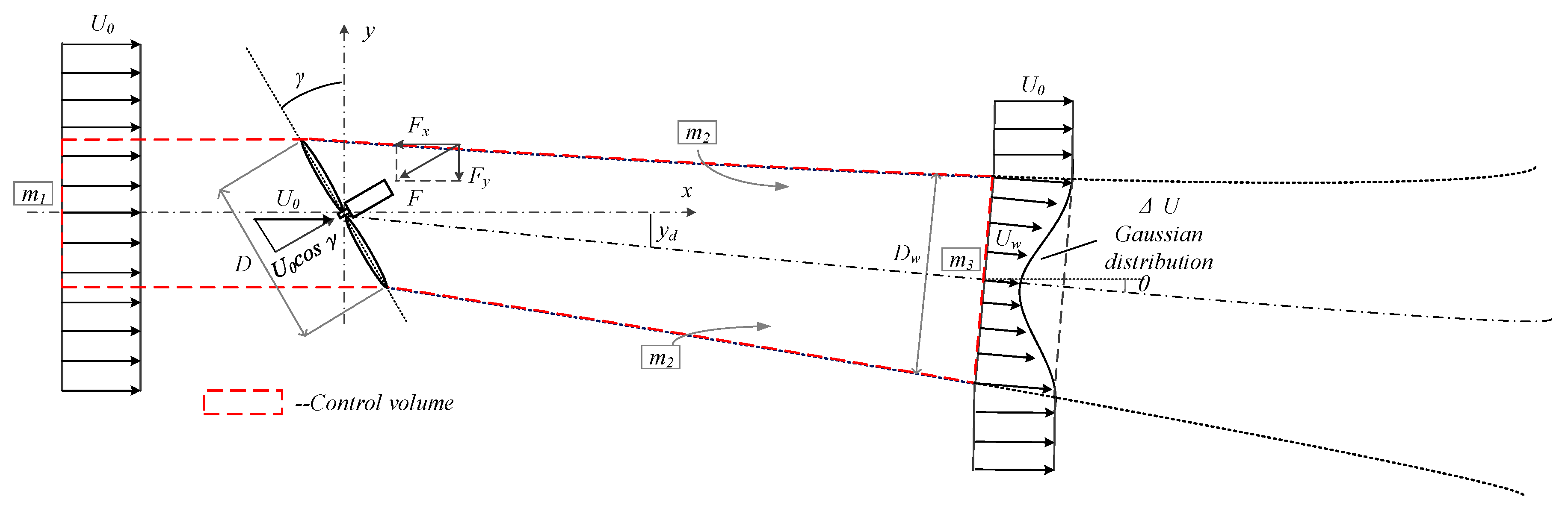
In this study, the Gaussian distribution function of velocity deficit is used together with the momentum conservation in the lateral direction to derive a new analytical wake deflection model. The model development is shown schematically in Figure 8, in which is the skew angle denoting the inclination angle of velocity in the wake with respect to the upstream velocity and the wake width is the spanwise distance between the two side boundaries. Similar to the basic approach of Jimenez et al. [11], the zone denoted by the red dashed lines is the control volume taken into account. It should be noted that to build the control volume, it is necessary to define a specific wake boundary. For simplification, the assumption of top-hat for the skew angle of the wake deflection is adopted and the wake width is defined as a function of ambient turbulence intensity and thrust coefficient, while Bastankhah and Porté-Agel took the assumption of Gaussian distribution for the skew angle. Based on the Gaussian distribution assumption for the velocity deficit, the wake half-width denotes the location where the velocity deficit equals the half the maximum value, and the velocity deficit normalized by the maximum value at the twice of half-width is 0.018. Accordingly, is used to represent the wake boundary denoted by the black dotted lines downstream the turbine. Here, is the representative wake width for a Gaussian distributed velocity deficit in the spanwise direction. In this study, the yaw angle is positive in the anti-clockwise direction, and the skew angle is positive in the clockwise direction from the top view.
The turbine induced force exerting on the control volume is supposed to be due only to the velocity component perpendicular to the rotor and it is expressed by the following equation:
The projections of this thrust force in streamwise and spanwise directions are expressed as:
As shown in Figure 8, is the mass flow crossing the wind turbine, is the flow entertainment into the wake and is the mass flow crossing the outlet of the control volume and is expressed as:
where is the velocity in the wake region.
By taking the momentum conservation in the control volume, the following relationship can be obtained:
The above equation can be decomposed into streamwise and spanwise components, respectively.
where the skew angle is small enough with the approximation of and in the far wake region.
From the mass conservation and substituting Equations (24) and (26) into Equation (28), the following relation can be derived for streamwise direction:
It is not difficult to find that the above equation has the same form with that under the non-yawed conditions if the transformation of is used. Thus, the formula of velocity deficit under the non-yawed conditions shown in the Appendix C is also applicable to that under the yawed conditions, and based on the self-similarity assumption the velocity in the wake region can be expressed as:
where and are the spanwise and streawise functions for velocity deficit. The Gaussian distribution is used for :
where is the distance from the wake center in the spanwise direction. The streamwise function in the far wake region can be obtained by taking the first order approximation of Taylor expansion for the solution derived by Bastankhah and Porté-Agel [36]
As mentioned above, the wake deflection is induced by the lateral force component, therefore the momentum equation in spanwise direction is analyzed to reveal the relationship between them. The skew angle is assumed to be constant within the assumed wake boundary. Then by equating Equations (25) and (29) and taking the approximation of , the expression of skew angle is obtained as:
Based on the above assumed wake boundary of , the integration in the above Equation (34) is calculated in the spanwise direction under a polar coordinate system with the origin at the wake center as follows:
By inserting Equations (32), (33) and (35) into Equation (34), the skew angle can be determined as:
As it is known, the skew angle is the derivative of the wake deflection:
Considering that the above derivation process is just applicable for the far wake region, Equation (37) is integrated from an initial far wake location to find the far wake deflection for as:
where is the wake deflection at and is replaced by based on the expression of as follows:
where and are the parameters with the function of and as shown in the Appendix C.
Then by substituting Equation (34) into Equation (38), the final expression for the far wake deflection is obtained as follows:
To complete the above model, the values of and also need to be determined. In this study, the wake deflection in the near wake region for is also assumed to be linear with the distance, and is expressed by:
where is the initial skew angle and it can be determined based on the approach of Coleman et al. [37]:
Note that the apparent difference between Equation (42) and the original formula is due to the different definition of thrust coefficients as shown in Equation (21).
For the value of and , Bastankhah and Porté-Agel [9] derived the onset of the far wake region based on the idealized potential core analysis. In this study, a simple method to find the value of and is derived from the mathematical viewpoint. The wake skew angle predicted in the near and far wake region should have the same value at the joint location, i.e., . Thus, by equating Equations (36) and (42), the value of can be directly obtained as:
The value of can be calculated based on Equation (39) as follows:
As noted by Bastankhah and Porté-Agel [9], the above estimation of does not aim to accurately predict the near wake length, but give an initial value for the far wake model.
Figure 9 shows the comparison between the wake deflections obtained from the experiment by Bastankhah and Porté-Agel [9] and those predicted by the models. In addition, the NRMSE of predicted result respect to the experimental data for each model are summarized in Table 4, in which the mean value of deflections from experimental data in the far wake region () is used for the normalization. Note that the corresponding shown in the figure for each case need to be replaced with for the calculation of Jiménez’s model and the proposed model since the thrust coefficient defined by Bastankhah and Porté-Agel [9] is different from Equation (21). It is found that, the Jiménez’s model generally overestimates the wake deflections. The proposed model denoted by solid red lines and the Bastankhah and Porté-Agel’s model plotted by blue dashed lines show good agreement with the experimental data. The parameter from the experimental data fitting is used for the Bastankhah and Porté-Agel’s model.
4.2. Wake Model for Yawed Wind Turbines
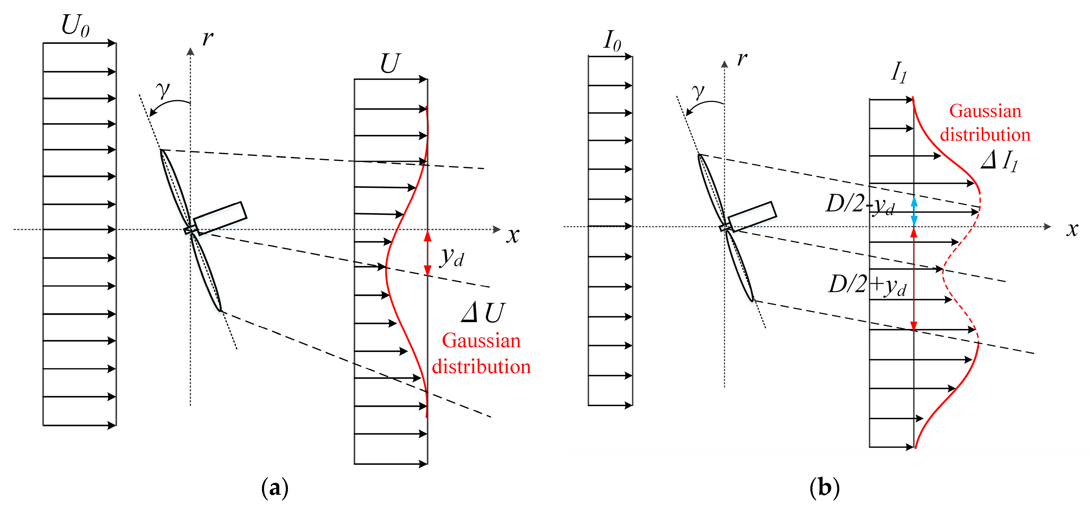
Figure 10 shows the schematic of wake model under yawed conditions for the velocity deficit and added turbulence intensity, in which and denote the upstream mean velocity and turbulence intensity. In order to incorporate the yawed condition into the wake model proposed by Qian and Ishihara [27], two basic assumptions are used in this study. One is to assume that the Gaussian distribution and self-similarity are applicable for the velocity deficit and added turbulence intensity distributions in cross-section of wake, and the other is to assume that the turbulence intensity distributions have the same wake deflections as those for the velocity deficit at each downwind location. Based on these assumptions, the wake model for the non-yawed wind turbines (see Equations (60) and (67) in Appendix C) is modified for the velocity deficit and added turbulence intensity prediction under yawed conditions:
where the is the trust coefficients under the yawed condition and is the distance from the wake center in the spanwise direction. They need to be replaced by the following expressions as mentioned at Section 4.1:
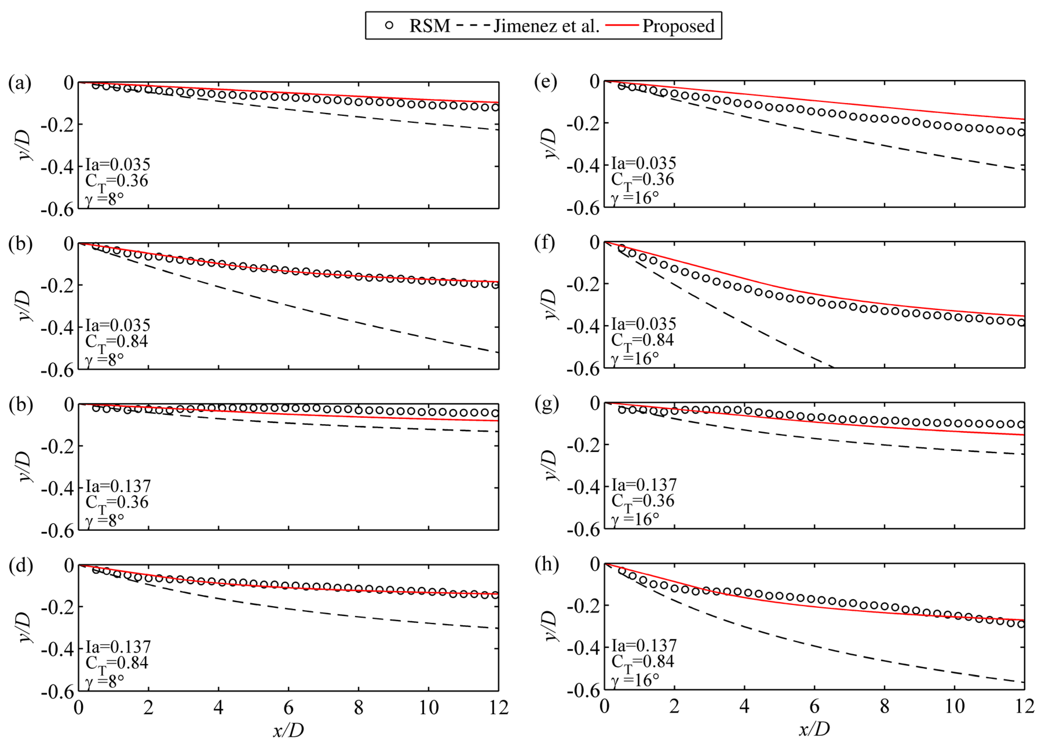
The parameters used in the wake model proposed by Qian and Ishihara [27] are shown in Appendix C. Figure 11 shows the wake deflections under the different conditions, in which the open circles denote the numerical results. The predicted values by Jimenez’s model and the proposed model are plotted by black dashed lines and red solid lines, respectively. The model of Bastankhah and Porté-Agel is not plotted since the parameters and have not been specified. It is noticed that the proposed model shows good agreement with the numerical results, however, the Jiménez’s model overestimates the deflections especially for the cases with the large thrust coefficients. In addition, it is clearly observed that the wake deflections increase almost linearly in the near wake region and then grow slowly in the far wake region. The slopes, i.e., wake skew angles are almost same for the cases with the same and under the same yaw angles. This justifies that Equations (41) and (42) are suitable for the initial wake deflection prediction by assuming a constant initial skew angle which just depends on the and the yaw angle . The high ambient turbulence generally decreases the length of potential core region and accelerates the flow mixing in the far wake region, whereby the wake deflections decrease. It can be inferred that the yaw control strategy is more efficient under low ambient turbulence such as in offshore wind farms.
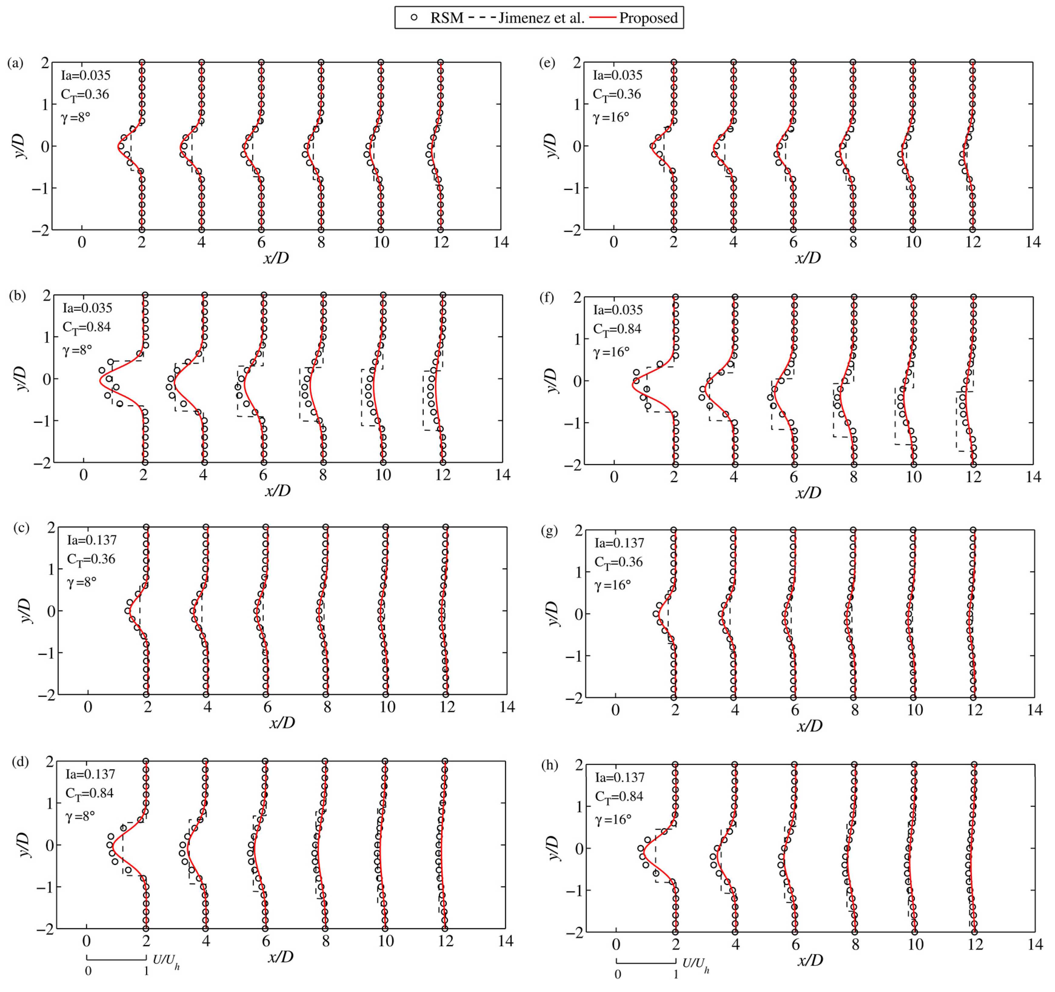
Figure 12 and Figure 13 show comparisons between the simulation results and the wake models for mean velocity and turbulence intensity, respectively. In these figures, the horizontal profiles of the normalized mean velocity and turbulence intensity at selected downwind locations of 2D, 4D, 6D, 8D, 10D and 12D are plotted. The numerical results are shown by the open circles and the red solid lines denote the results predicted by the proposed model. The x-axis illustrates the distance from the wind turbine normalized by the rotor diameter D. The distance of 2D corresponds to a unit scale of normalized mean velocity in Figure 12 and a scale of turbulence intensity with the value of 0.3 in Figure 13, respectively. In Figure 12, the mean velocity predicted by the Jiménez’s model is also plotted by black dashed lines for comparison. The velocity deficit for this model is calculated with the top-hat model proposed by Katic et al. [38]:
where is the wake decay factor and the recommended values is for the flat terrain under the neutral conditions [39].
As shown in Figure 12, the proposed model gives more accurate predictions for the mean velocity distributions under the different yawed conditions than those by the top-hat shape used in the Jimenez’s model, which underestimates the velocity deficit in the center of the wake and overestimates them in the outside regions.
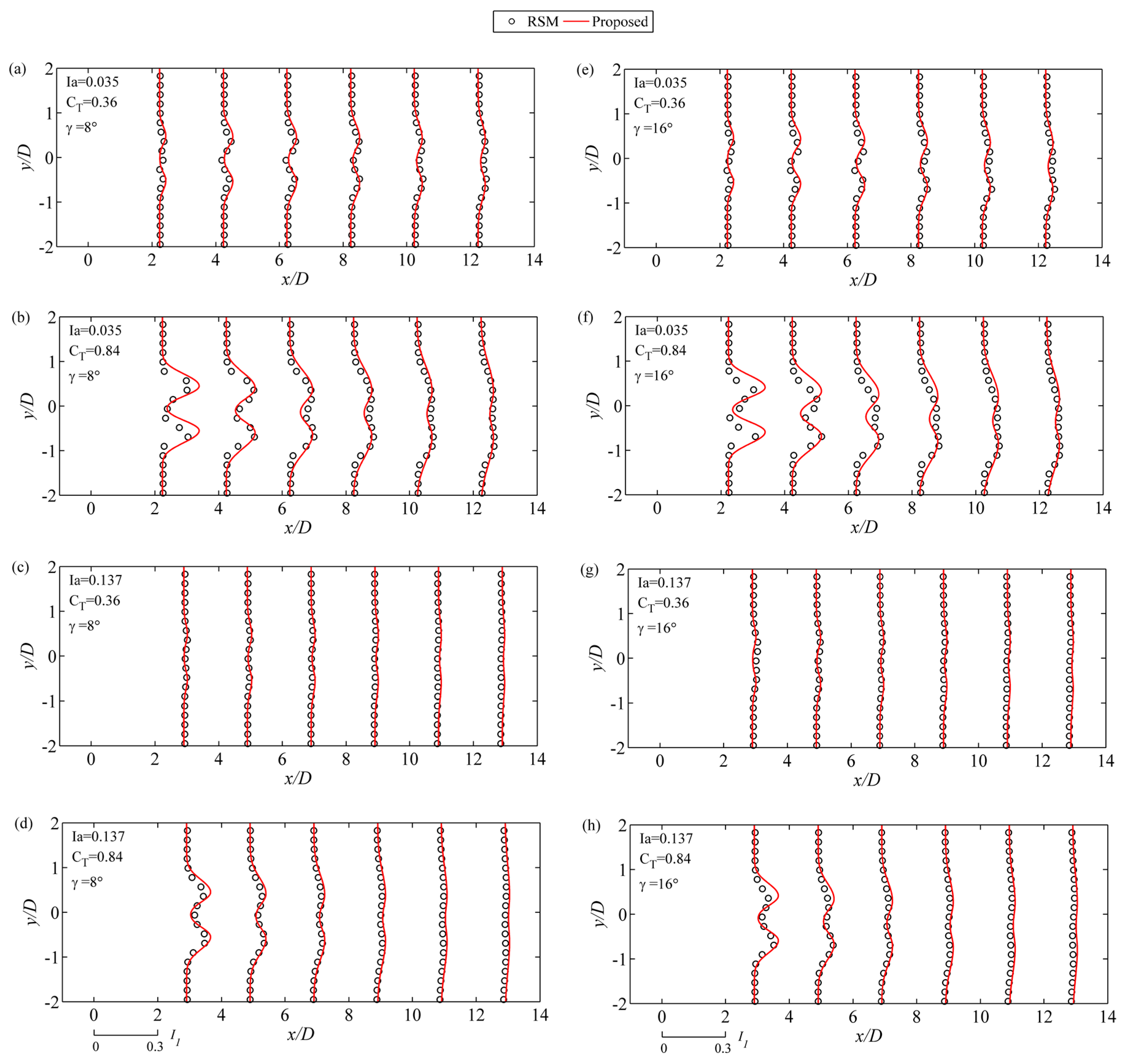
Since the turbulence intensity prediction was not included in the previous wake models proposed by Jimenez et al. [11] and Bastankhah and Porté-Agel [9], only turbulence intensities by the proposed model in this study are plotted for comparison with the numerical results. As shown in Figure 13, the proposed model satisfactorily predicts the turbulence intensity distribution in the wake of yawed turbines. It is noticed that the predicted mean velocity and turbulence intensity distributions in the spanwise direction are assumed symmetric to the wake center trajectory, while the profiles of mean velocity and turbulence intensity from the numerical simulations present slightly skewed shape as shown in Figure 12 and Figure 13.
5. Conclusions
In this study, a systematic numerical simulation for wind turbine wakes with different ambient turbulence intensities, thrust coefficients, and yaw angles is carried out by using the Reynolds Stress Model. A new analytical wake deflection model is developed based on the theoretical analysis of turbine induced force and the momentum conservation for a control volume around the yawed turbine. The proposed wake deflection model is incorporated into the previous wake model to predict the mean velocity and turbulence intensity in the wake region. Following conclusions are obtained:
- The numerical results by using the Reynolds Stress Model show good agreement with those by LES model. Based on a systematic numerical simulation, it is found that the high turbulence accelerates the process of flow mixing in the wake region, thus wake deflection recover faster than those with the low ambient turbulence intensity.
- A new analytical wake deflection model is proposed based on the Gaussian distribution for velocity deficit and the top-hat shape for skew angle and it is validated by comparison with the results obtained from the wind tunnel test and the numerical simulations. The model parameters are determined as the function of ambient turbulence intensity and thrust coefficient, which enables the model to have good applicability under various conditions.
- An analytical wake model for the yawed wind turbines is developed by incorporating the proposed wake deflection model, which shows good performance for predicting distributions of mean velocity and turbulence intensity by comparison with the numerical results.
Acknowledgments
This research was carried out as a part of the project funded by Hitachi, Ltd. and ClassNK. The authors express their deepest gratitude to the concerned parties for their assistance during this study.
Author Contributions
This study was done as a part of Guo-Wei Qian’s doctoral research supervised by Takeshi Ishihara. Guo-Wei Qian and Takeshi Ishihara designed the structure of the paper and wrote the paper.
Conflicts of Interest
The authors declare no conflict of interest.
Appendix A. Wake Defection Model of Jimenez et al.
Based on the momentum conservation and top-hat assumption for velocity deficit, the wake skew angle is proposed by Jimenez et al. [11] as follows:
which is assumed to be constant in the spanwise direction within the wake boundary. is the wake expansion factor and the recommend values is for the flat terrain under neutral conditions [39].
As shown by Gebraad et al. [5] and Howland et al. [40], the wake deflection was determined by integrating the skew angle in and using :
The top-hat velocity deficit model can be combined with this deflection model to predict the velocity field in yawed conditions. However, this model overestimates the wake deflection since the assumption of top-hat for the wake deficit is not accurate as pointed out by Ishihara et al. [18].
Appendix B. Wake Deflection Model by Bastankhah and Porté-Agel
In the near-wake region, the initial skew angle at the rotor is derived based on the approach of Coleman et al. [37] and is given by:
The length of the hypothetical potential core is expressed by
where , . The wake width at has the following expression,
As the wake skew angle is assumed to be constant in the potential core region, the value of deflection at is written as:
In the far-wake region, the wake deflection was determined as follows:
where and are the wake width in horizontal and vertical direction and expressed as:
It should be noted that the parameters and have no specific formulas, which implies that the model by Bastankhah and Porté-Agel [9] could not be generally applied in wake prediction under various conditions.
Appendix C. Wake Model for Non-Yawed Wind Turbines by Qian and Ishihara
A Gaussian-based analytical wake model in non-yawed condition, as shown in Figure 10 when the yaw angle equals 0, are proposed as follows:
The velocity deficit induced by the rotor is assumed to be axi-symmetric and self-similar following the spanwise function with a Gaussian shape in each wake cross section. They are expressed by the following equations:
where is the mean velocity in the wake region, is the upstream mean velocity, is the rotor diameter and is the radial distance form the center of the wake, is the standard deviation of the velocity deficit distribution at each cross section and is treated as the wake representative width. representing the maximum normalized velocity deficit occurring at the wake center is modeled as the function of and :
where and are the model parameters and is a correction term proposed to consider the velocity deficit in the new wake region and they are given by:
The wake region is assumed to expand linearly and is expressed by the following equations:
The added turbulence intensity is also assumed axi-symmetric and self-similar following the supposed spanwise function with a dual-Gaussian shape. They are described by the following equations:
where is the turbulence intensity in the wake region, is the upstream turbulence intensity. is the standard deviation of the added turbulence intensity at each cross section and it can be determined by the same expression as Equation (64). and are the parameters to combine the added turbulence intensity induced by each tip side with the expressions as follows:
denotes the maximum added turbulence intensity occurring at the tip side position, which is also modeled as the function of and :
References
- Adaramola, M.S.; Krogstad, P.-Å. Experimental investigation of wake effects on wind turbine performance. Renew. Energy 2011, 36, 2078–2086. [Google Scholar] [CrossRef]
- Wagenaar, J.W.; Machielse, L.A.H.; Schepers, J.G. Controlling Wind in ECN’s Scaled Wind Farm. In Proceedings of the European Wind Energy Association 2012, Copenhagen, Denmark, 16–19 April 2012. [Google Scholar]
- Mikkelsen, T.; Angelou, N.; Hansen, K.; Sjöholm, M.; Harris, M.; Slinger, C.; Hadley, P.; Scullion, R.; Ellis, G.; Vives, G. A spinner-integrated wind lidar for enhanced wind turbine control. Wind Energy 2013, 16, 625–643. [Google Scholar] [CrossRef] [Green Version]
- Medici, D.; Dahlberg, J.Å. Potential improvement of wind turbine array efficiency by active wake control (AWC). In Proceedings of the European Wind Energy Conference and Exhibition, Madrid, Spain, 16–19 June 2003; Department of Mechanics, The Royal Institute of Technology: Gottingen, Germany, 2003; pp. 65–84. [Google Scholar]
- Gebraad, P.M.O.; Teeuwisse, F.W.; van Wingerden, J.W.; Fleming, P.A.; Ruben, S.D.; Marden, J.R.; Pao, L.Y. Wind plant power optimization through yaw control using a parametric model for wake effects-a CFD simulation study. Wind Energy 2014, 19, 95–114. [Google Scholar] [CrossRef]
- Parkin, P.; Holm, R.; Medici, D. The application of PIV to the wake of a wind turbine in yaw. In Particle Image Velocimetry; Deptartment of mechanics, The Royal Institute of Technology: Gottingen, Germany, 2001. [Google Scholar]
- Medici, D.; Alfredsson, P.H. Measurements on a wind turbine wake: 3D effects and bluff body vortex shedding. Wind Energy 2006, 9, 219–236. [Google Scholar] [CrossRef]
- Howland, M.F.; Bossuyt, J.; Martinez-Tossas, L.A.; Meyers, J.; Meneveau, C. Wake Structure of Wind Turbines in Yaw under Uniform Inflow Conditions. arXiv, 2016; arXiv:1603.06632. [Google Scholar]
- Bastankhah, M.; Porté-Agel, F. Experimental and theoretical study of wind turbine wakes in yawed conditions. J. Fluid Mech. 2016, 806, 506–541. [Google Scholar] [CrossRef]
- Sanderse, B.; DerPijl, S.P.; Koren, B. Review of computational fluid dynamics for wind turbine wake aerodynamics. Wind Energy 2011, 14, 799–819. [Google Scholar] [CrossRef]
- Jiménez, Á.; Crespo, A.; Migoya, E. Application of a LES technique to characterize the wake deflection of a wind turbine in yaw. Wind Energy 2009, 13, 559–572. [Google Scholar] [CrossRef]
- Fleming, P.A.; Gebraad, P.M.O.; Lee, S.; van Wingerden, J.W.; Johnson, K.; Churchfield, M.; Michalakes, J.; Spalart, P.; Moriarty, P. Evaluating techniques for redirecting turbine wakes using SOWFA. Renew. Energy 2014, 70, 211–218. [Google Scholar] [CrossRef]
- Luo, L.; Srivastava, N.; Ramaprabhu, P. A Study of Intensified Wake Deflection by Multiple Yawed Turbines based on Large Eddy Simulations. In Proceedings of the 33rd Wind Energy Symposium, Kissimmee, FL, USA, 5–9 January 2015; pp. 1–19. [Google Scholar] [CrossRef]
- Crespo, A.; Hernández, J.; Frandsen, S. Survey of modelling methods for wind turbine wakes and wind farms. Wind Energy 1999, 2, 1–24. [Google Scholar] [CrossRef]
- Stevens, R.J.A.M.; Gayme, D.F.; Meneveau, C. Coupled wake boundary layer model of wind-farms. J. Renew. Sustain. Energy 2015, 7. [Google Scholar] [CrossRef]
- Yang, X.; Sotiropoulos, F. Analytical model for predicting the performance of arbitrary size and layout wind farms. Wind Energy 2016, 19, 1239–1248. [Google Scholar] [CrossRef]
- Jensen, N.O. A Note on Wind Generator Interaction; Risø National Laboratory: Roskilde, Denmark, 1983; ISBN 87-550-0971-9. [Google Scholar]
- Ishihara, T.; Yamaguchi, A.; Fujino, Y. Development of a New Wake Model Based on a Wind Tunnel Experiment. Glob. Wind Power 2004. Available online: http://windeng.t.u-tokyo.ac.jp/ishihara/e/proceedings/2004-5_poster.pdf (accessed on 7 March 2018).
- Cabezón, D.; Migoya, E.; Crespo, A. Comparison of turbulence models for the computational fluid dynamics simulation of wind turbine wakes in the atmospheric boundary layer. Wind Energy 2011, 14, 909–921. [Google Scholar] [CrossRef] [Green Version]
- Ansys Inc. ANSYS Fluent Theory Guide; Ansys Inc.: Canonsburg, PA, USA, 2011. [Google Scholar]
- Lien, F.; Leschziner, M. Assessment of turbulence-transport models including non-linear rng eddy-viscosity formulation and second-moment closure for flow over a backward-facing step. Comput. Fluids 1994, 23, 983–1004. [Google Scholar] [CrossRef]
- Gibson, M.M.; Launder, B.E. Ground effects on pressure fluctuations in the atmospheric boundary layer. J. Fluid Mech. 1978, 86, 491. [Google Scholar] [CrossRef]
- Fu, S.; Launder, B.E.; Leschziner, M.A. Modelling strongly swirling recirculating jet flow with Reynolds-stress transport closures. In Proceedings of the 6th Symposium on Turbulent Shear Flows, Toulouse, France, 7–9 September 1987; Proceedings (A88-38951 15-34). Pennsylvania State University: University Park, PA, USA, 1987; pp. 17-6-1–17-6-6. [Google Scholar]
- Launder, B.E. Second-moment closure: Present … and future? Int. J. Heat Fluid Flow 1989, 10, 282–300. [Google Scholar] [CrossRef]
- Launder, B.E. Second-moment closure and its use in modelling turbulent industrial flows. Int. J. Numer. Methods Fluids 1989, 9, 963–985. [Google Scholar] [CrossRef]
- Ferziger, J.H.; Perić, M. Computational Methods for Fluid Dynamics; Springer: New York, NY, USA, 2002; ISBN 9783540420743. [Google Scholar]
- Qian, G.-W.; Ishihara, T. A Numerical Study of Wind Turbine Wake by Large Eddy Simulation and Proposal for a New Analytical Wake Model. In Proceedings of the Offshore Wind Energy, London, UK, 6–8 June 2017. [Google Scholar]
- Burton, T.; Sharpe, D.; Jenkins, N.; Bossanyi, E. Wind Energy Handbook, 2nd ed.; Wiley: New York, NY, USA, 2011; ISBN 9780470699751. [Google Scholar]
- Glauert, H. The Analysis of Experimental Results in the Windmill Brake and Vortex Ring States of an Airscrew; HMSO: London, UK, 1926. [Google Scholar]
- Haans, W. Wind Turbine Aerodynamics in Yaw: Unravelling the Measured Rotor Wake. Ph.D. Thesis, Delft University of Technology, Delft, The Netherlands, 2011. [Google Scholar]
- Dörenkämper, M.; Witha, B.; Steinfeld, G.; Heinemann, D.; Kühn, M. The impact of stable atmospheric boundary layers on wind-turbine wakes within offshore wind farms. J. Wind Eng. Ind. Aerodyn. 2015, 144, 146–153. [Google Scholar] [CrossRef]
- Wu, Y.-T.; Porté-Agel, F. Modeling turbine wakes and power losses within a wind farm using LES: An application to the Horns Rev offshore wind farm. Renew. Energy 2015, 75, 945–955. [Google Scholar] [CrossRef]
- Vollmer, L.; Steinfeld, G.; Heinemann, D.; Kühn, M. Estimating the wake deflection downstream of a wind turbine in different atmospheric stabilities: An LES study. Wind Energ. Sci. 2016, 1, 129–141. [Google Scholar] [CrossRef]
- The International Electrotechnical Commission (IEC). IEC 61400-1:2005+AMD1:2010, Wind Turbines—Part 1: Design Requirements; IEC: Geneva, Switzerland, 2014. [Google Scholar]
- Wikipedia. Available online: https://en.wikipedia.org/wiki/Root-mean-square_deviation (accessed on 19 February 2018).
- Bastankhah, M.; Porté-Agel, F. A new analytical model for wind-turbine wakes. Renew. Energy 2014, 70, 116–123. [Google Scholar] [CrossRef]
- Coleman, R.P.; Feingold, A.M. Evaluation of the Induced-Velocity Field of an Idealized Helicoptor Rotor; Wartime Report; UNT: Denton, TX, USA, 1945; p. 28. [Google Scholar]
- Katic, I.; Hojstrup, J.; Jensen, N.O. A simple model for cluster efficiency i.katic. j.højstrup. n.o.jensen. In Proceedings of the European Wind Energy Association, Rome, Italy, 7–9 October 1986; pp. 407–410. [Google Scholar]
- Peña, A.; Réthoré, P.-E.; van der Laan, M.P. On the application of the Jensen wake model using a turbulence-dependent wake decay coefficient: The Sexbierum case. Wind Energy 2016, 19, 763–776. [Google Scholar] [CrossRef] [Green Version]
- Howland, M.F.; Bossuyt, J.; Martínez-Tossas, L.A.; Meyers, J.; Meneveau, C.; Mart Inez-Tossas, L.A. Wake structure in actuator disk models of wind turbines in yaw under uniform inflow conditions. J. Renew. Sustain. Energy 2016, 8. [Google Scholar] [CrossRef]
Figure 1.
Schematic of the ADM-R model for the yawed rotor: (a) isometric view, (b) top view.
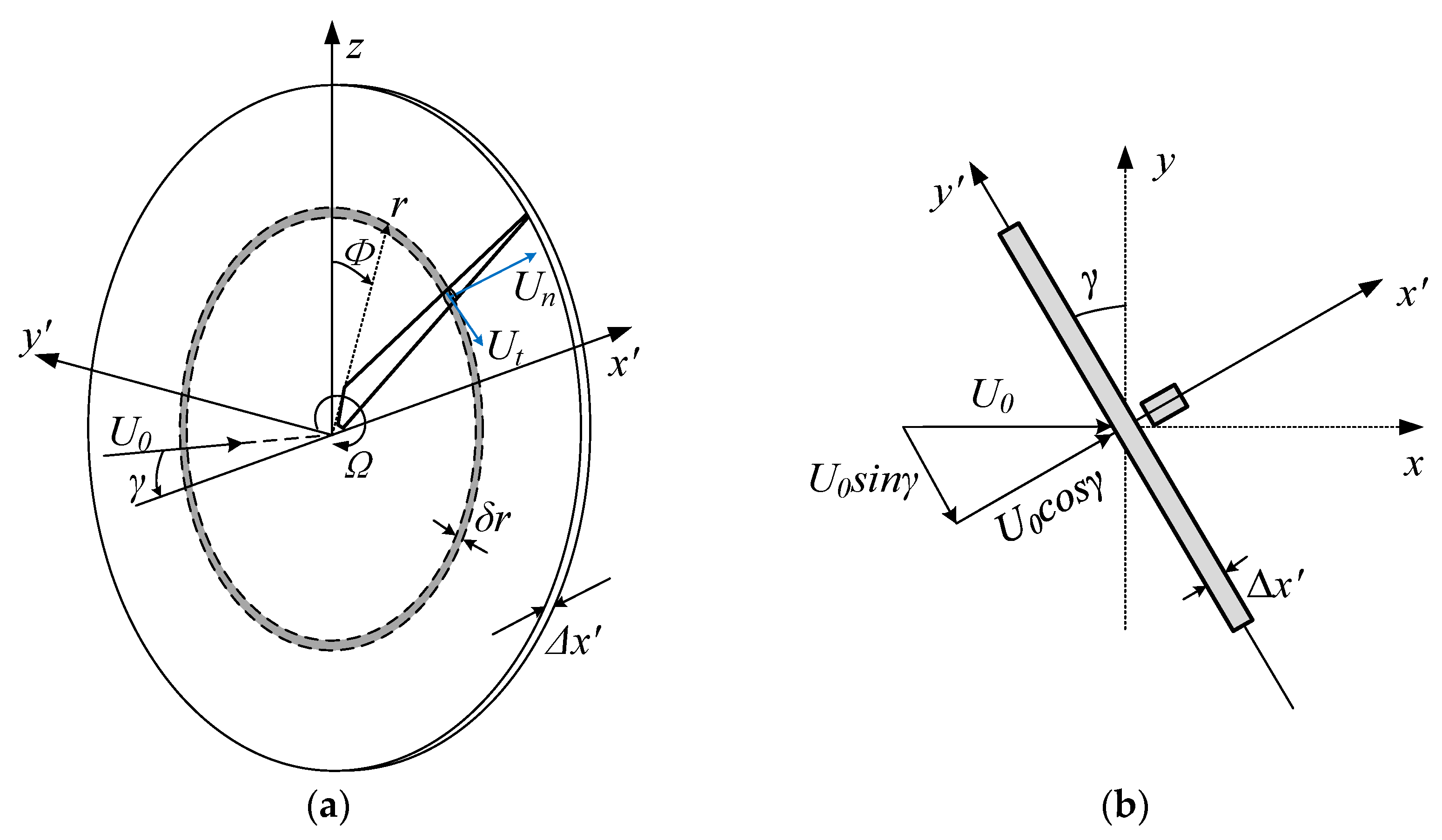
Figure 2.
Velocities and forces acting on a cross-sectional blade element.
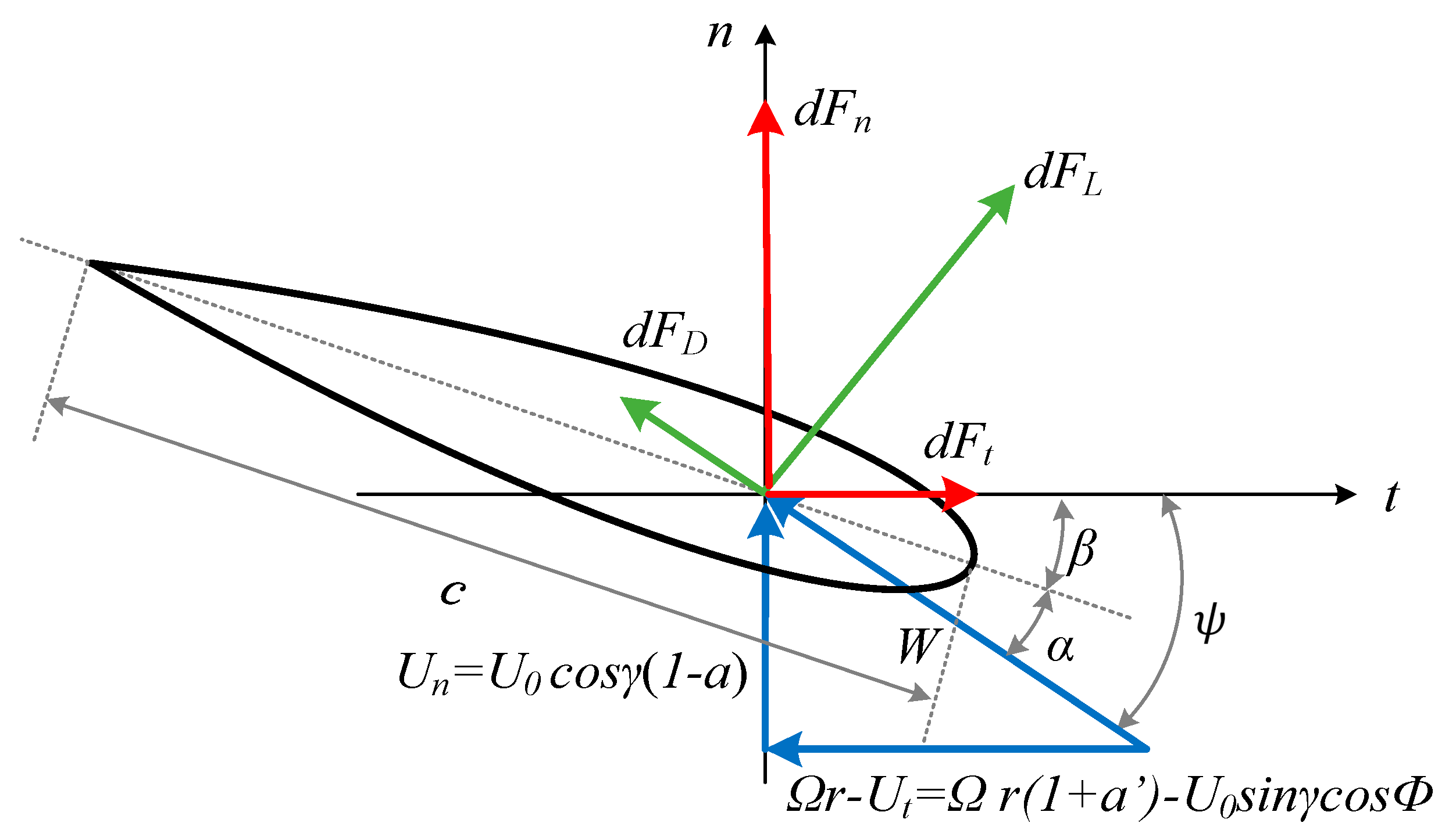
Figure 3.
Schematic view of the computational domain.

Figure 4.
Vertical profiles in the simulated neutral atmospheric boundary layers without wind turbines: (a,c) for normalized mean velocity; (b,d) for turbulence intensity.
Figure 4.
Vertical profiles in the simulated neutral atmospheric boundary layers without wind turbines: (a,c) for normalized mean velocity; (b,d) for turbulence intensity.
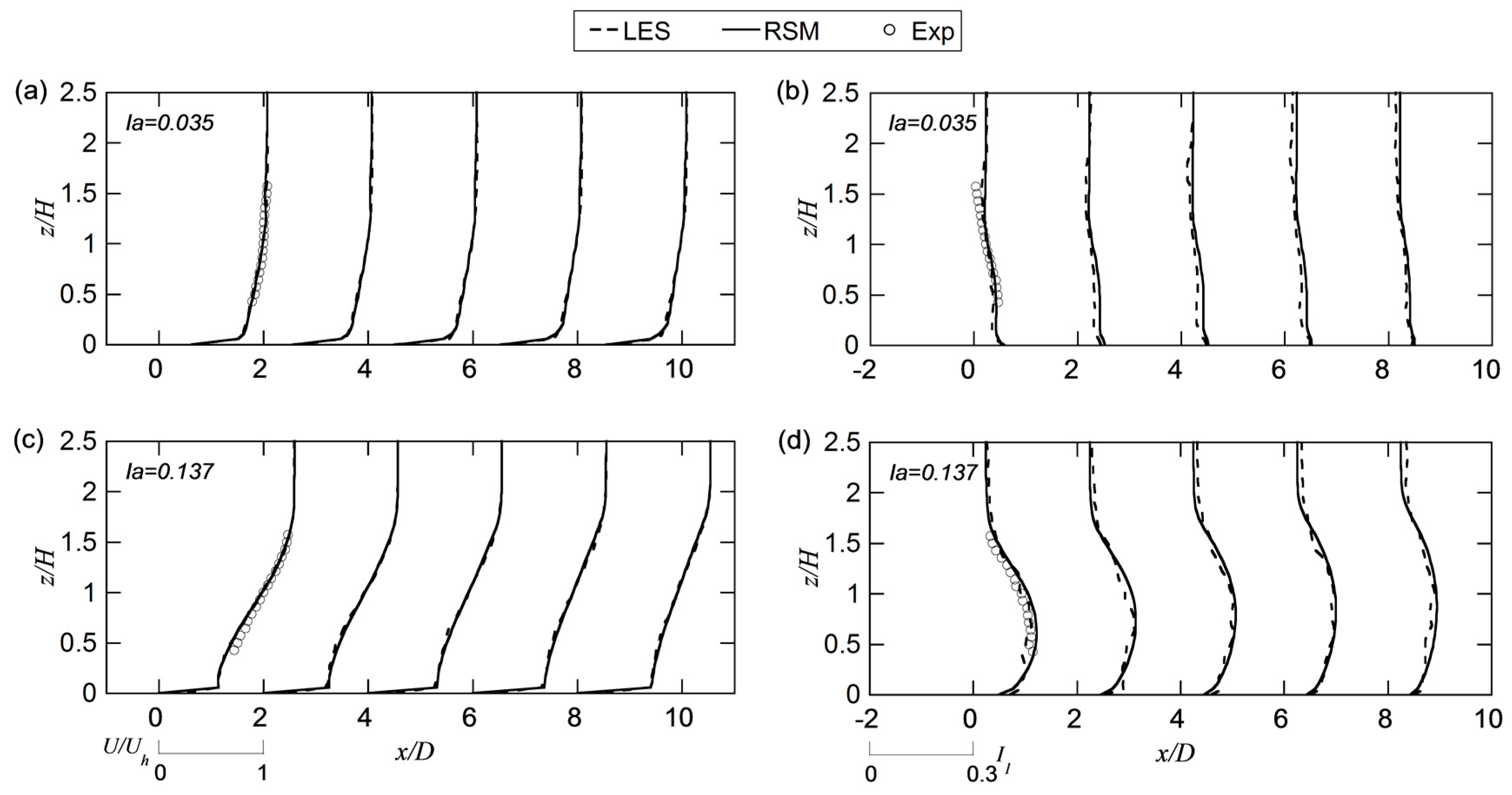
Figure 5.
Wake characteristics in the horizontal x-y plane at hub height under non-yawed conditions: (a,c) for normalized mean velocity; (b,d) for turbulence intensity.
Figure 5.
Wake characteristics in the horizontal x-y plane at hub height under non-yawed conditions: (a,c) for normalized mean velocity; (b,d) for turbulence intensity.

Figure 6.
Contours of normalized mean velocity and wake deflections in the horizontal x-y plane at the hub height. Solid lines represent the wind turbine rotors. Dashed lines and open circles indicate the wake boundaries and wake center trajectories, respectively.
Figure 6.
Contours of normalized mean velocity and wake deflections in the horizontal x-y plane at the hub height. Solid lines represent the wind turbine rotors. Dashed lines and open circles indicate the wake boundaries and wake center trajectories, respectively.
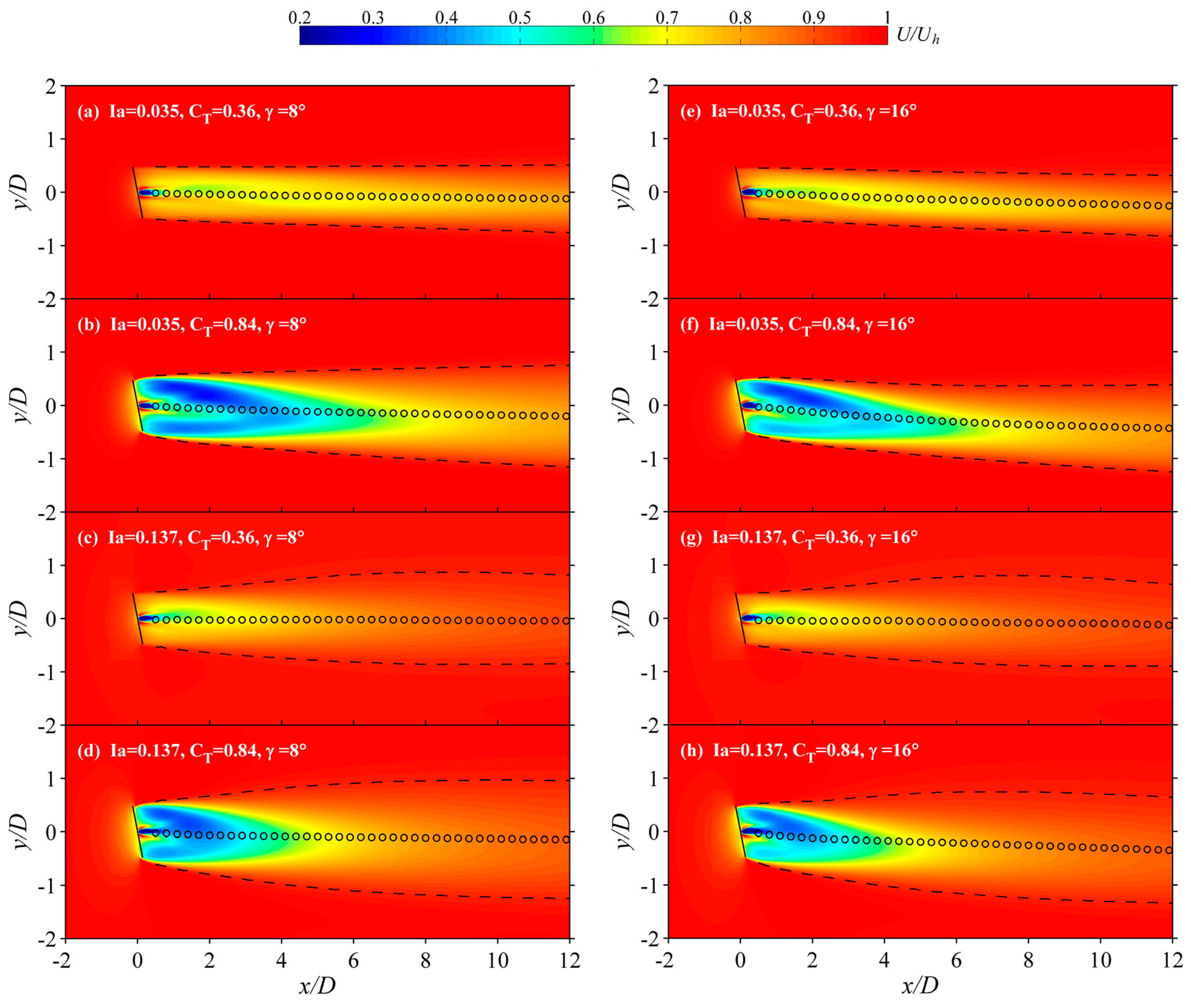
Figure 7.
Contours of turbulence intensity and wake deflections in the horizontal x-y plane at the hub height. Solid lines represent the wind turbine rotors. Dashed lines denote the position of peak values of turbulence intensity and the midpoint of the two peaks are indicated by the open circles. The wake center trajectories obtained from the mean velocity contours are plotted by red dotted lines.

Figure 8.
Schematic of the momentum conservation-based model for the wake deflection. Black dotted lines downstream the turbine represent the wake boundaries and the part overlapped by the red dashed lines are used to establish the control volume.
Figure 8.
Schematic of the momentum conservation-based model for the wake deflection. Black dotted lines downstream the turbine represent the wake boundaries and the part overlapped by the red dashed lines are used to establish the control volume.

Figure 9.
Comparison between wake deflection models and the experiment results.
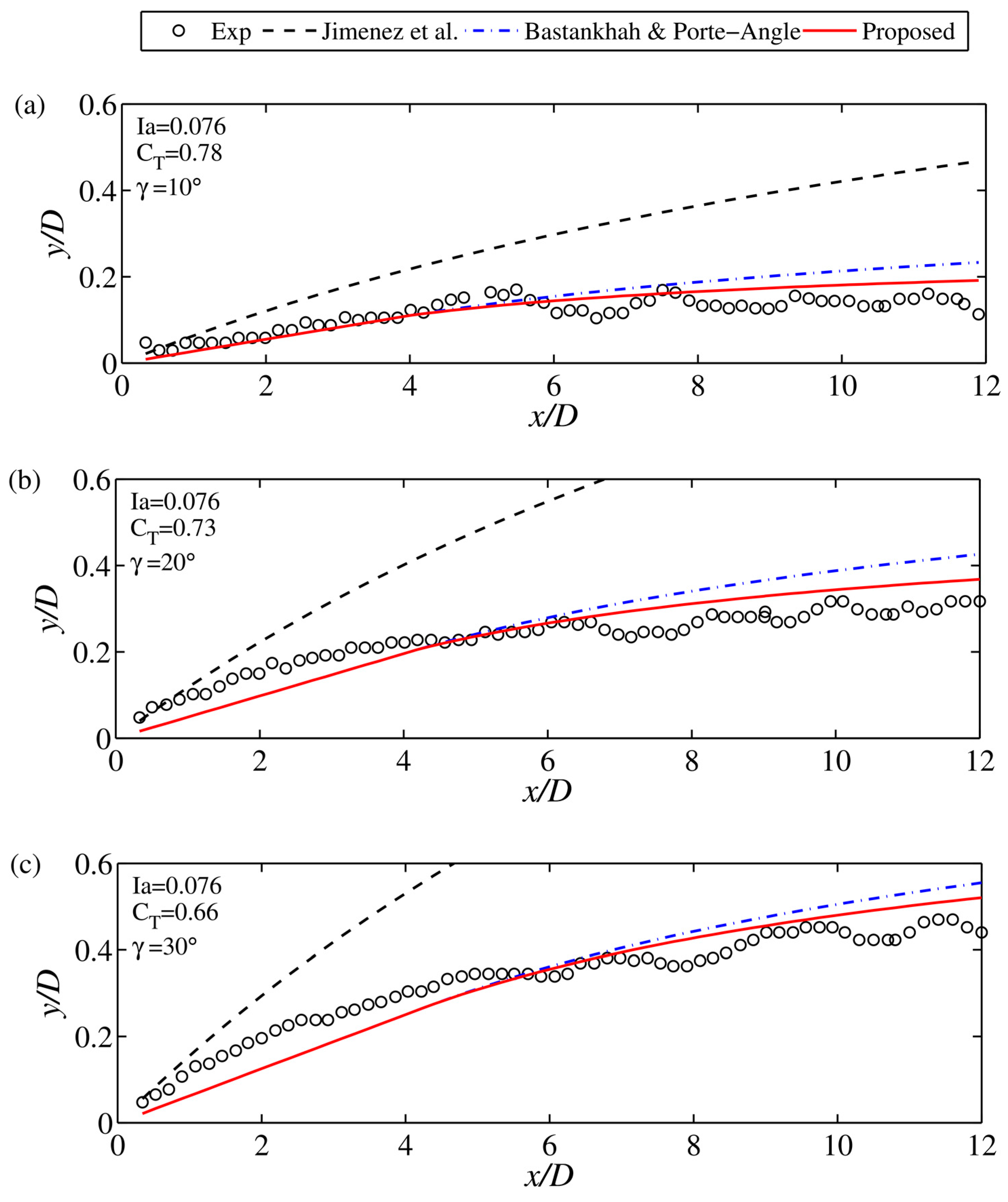
Figure 10.
Schematic of the Gaussian-based wake model in yawed condition: (a) mean velocity (b) turbulence intensity.
Figure 10.
Schematic of the Gaussian-based wake model in yawed condition: (a) mean velocity (b) turbulence intensity.

Figure 11.
Validation for predicted wake deflections in yawed conditions.

Figure 12.
Validation for the predicted mean velocity under the yawed conditions.

Figure 13.
Validation for the predicted turbulence intensity in the yawed conditions.

Table 1.
Boundary conditions.
| Boundary | Specification |
|---|---|
| Inlet | Profiles of |
| Outlet | Outflow |
| Side | Symmetry |
| Top | Symmetry |
| Bottom | Logarithmic law |
Table 2.
Parameters of numerical simulation.
| Case | (Deg.) | ||
|---|---|---|---|
| 1 | 8 | 0.035 | 0.36 |
| 2 | 8 | 0.035 | 0.84 |
| 3 | 8 | 0.137 | 0.36 |
| 4 | 8 | 0.137 | 0.84 |
| 5 | 16 | 0.035 | 0.36 |
| 6 | 16 | 0.035 | 0.84 |
| 7 | 16 | 0.137 | 0.36 |
| 8 | 16 | 0.137 | 0.84 |
Table 3.
NRMSE of simulated profiles respect to experimental data: Inflow for the result in Figure 4 and Wake flow for the result in Figure 5.
| Inflow | |||||
| LES | 0.012 | 0.24 | 0.031 | 0.10 | |
| RSM | 0.015 | 0.26 | 0.032 | 0.13 | |
| Wake flow | , | , | |||
| LES | 0.068 | 0.078 | 0.071 | 0.12 | |
| RSM | 0.078 | 0.075 | 0.074 | 0.10 | |
Table 4.
NRMSE of predicted wake deflections.
| Model | |||
|---|---|---|---|
| Jiménez | 1.38 | 1.16 | 0.94 |
| Bastankhah and Porté-Agel | 0.31 | 0.23 | 0.13 |
| Proposed | 0.29 | 0.20 | 0.11 |
© 2018 by the authors. Licensee MDPI, Basel, Switzerland. This article is an open access article distributed under the terms and conditions of the Creative Commons Attribution (CC BY) license (http://creativecommons.org/licenses/by/4.0/).
Share and Cite
MDPI and ACS Style
Qian, G.-W.; Ishihara, T. A New Analytical Wake Model for Yawed Wind Turbines. Energies 2018, 11, 665. https://doi.org/10.3390/en11030665
AMA Style
Qian G-W, Ishihara T. A New Analytical Wake Model for Yawed Wind Turbines. Energies. 2018; 11(3):665. https://doi.org/10.3390/en11030665
Chicago/Turabian StyleQian, Guo-Wei, and Takeshi Ishihara. 2018. "A New Analytical Wake Model for Yawed Wind Turbines" Energies 11, no. 3: 665. https://doi.org/10.3390/en11030665
Note that from the first issue of 2016, this journal uses article numbers instead of page numbers. See further details here.