Optimal Sizing and Location of Distributed Generators Based on PBIL and PSO Techniques

Abstract

The optimal location and sizing of distributed generation is a suitable option for improving the operation of electric systems. This paper proposes a parallel implementation of the Population-Based Incremental Learning (PBIL) algorithm to locate distributed generators (DGs), and the use of Particle Swarm Optimization (PSO) to define the size those devices. The resulting method is a master-slave hybrid approach based on both the parallel PBIL (PPBIL) algorithm and the PSO, which reduces the computation time in comparison with other techniques commonly used to address this problem. Moreover, the new hybrid method also reduces the active power losses and improves the nodal voltage profiles. In order to verify the performance of the new method, test systems with 33 and 69 buses are implemented in Matlab, using Matpower, for evaluating multiple cases. Finally, the proposed method is contrasted with the Loss Sensitivity Factor (LSF), a Genetic Algorithm (GA) and a Parallel Monte-Carlo algorithm. The results demonstrate that the proposed PPBIL-PSO method provides the best balance between processing time, voltage profiles and reduction of power losses.

1. Introduction

In recent years, grid operators have been forced by new regulations and incentives imposed by grid regulators to improve the operating conditions of their electrical grids, such as power losses, voltage profiles, line loadability and harmonic distortion index [1]. For this reason, several works have been carried out to improve the technical conditions of electrical grids with the lowest investment possible [2]. Some of those solutions include the reconfiguration of the Distribution System (DS) [3], the installation of capacitor banks [4], implementation of solid-state synchronous compensators [5], installation of voltage regulators [6], integration of energy storage systems [7] and the installation of Distributed Generators (DGs) [8]. In particular, the integration of DGs into an electrical grid is, nowadays, strongly discussed because it enables the combination of conventional and non-conventional (renewable) energy sources.

The installation of DGs in a DS has been extensively discussed in literature [2,9,10]. Moreover, those works have also discussed the improvements provided by DSs into the technical criteria of the grid and, as additional product, the reduction of the pollution caused by oil-based generation [11,12]: reduction of power losses (due to transmission), improvement of voltage profiles and stability index, power factor enhancement, reduction of the harmonic distortion and increased line loadability, among others [13]. However, incorrect location or sizing procedures may result in voltage profiles out of conventional ranges, voltage fluctuations, line capacity violation, increased failure levels due to intermittent generation and higher costs associated to the DGs [14].

Different methods have been developed to optimize the location and sizing of DGs. Those methods are aimed at reducing the computation time required and to improve the technical criteria of the grid, such as power losses, voltage profiles and power factor, among others [15,16]. For example, the work reported in [17] presents a hybrid method between the genetic algorithm proposed by Chu and Beasley (GACB) [18] and a heuristic approach to locate, select and size the feeders in a distributed generation environment. Such a strategy enables the reduction of the costs associated with the feeders (DGs) and the power losses, which is achieved by reducing the peak load using active power injection based on diesel-based DGs only. On the other hand, the work reported in [19] describes a multi-target approach based on the Particle Swarm Optimization (PSO) technique for locating the DGs, and an optimal flow analysis for sizing the DGs. That work considers several generators and different load models, thus enabling high penetration levels of distributed generation.

A similar approach was presented in [20], which is a hybrid solution based on both the GACB and PSO. The main drawbacks of such a solution were the high level of power injection requested to the DGs and the lack of analysis of the computation time required by the proposed method. Another solution, based on the Loss Sensitivity Factor (LSF) for location and the Bacterial Foraging Optimization Algorithm (BFOA) for sizing was introduced in [21]. The adoption of a heuristic technique for the generator location ensured a reduced computation burden in comparison with previous solutions, however, the solution space is not optimally explored, and hence the method could be trapped into a local optima. Another application of the PSO algorithm in a DGs location process was reported in [22]. In that work the authors propose a modified PSO algorithm to locate photovoltaic generators and capacitors in a grid, applying an additional Monte Carlo algorithm to define the generators size, hence, its main objective is to reduce the power losses and to improve the voltage profiles.

Other optimization techniques have been used to design DGs systems. For example, the work reported in [23] proposes a hybrid method based on the Ant Colony Optimization (ACO) and Artificial Bee Colony (ABC) techniques to integrate renewable energy sources into the grid. In that work the objective functions of the optimization problem were defined to reduce the power losses, to improve the voltage profiles and to reduce the pollution. However, the work does not provide an analysis of the computation time required by the algorithm, which is a key factor to identify the computational cost of the proposed method [15]. Similarly, an algorithm based on Chaotic Symbiotic Organism Search (CSOS) for the location and sizing of DGs is presented in [24]. The main drawback of this solution is the exponential increment of the computation time when the exploration space is expanded. Finally, the adoption of the Ant Lion Optimization Algorithm (ALOA) for integrating wind and photovoltaic generators into the grid was reported in [25]. That solution is based on a sensitivity indicator for locating the devices, which enables the method to reduce the power losses and improve the voltage stability profiles by injecting power profiles close to the slack node without DGs.

The previous state-of-the-art reveals that integrating DGs into the DS requires the solution of two main problems: a binary decision problem focused on the DGs location (installing, or not, generators at the system buses) and a continuous problem focused on the DGs size (amount of power to be injected by the generators). Several of the methods adopted to define the DGs size do not limit the maximum power injected by the DGs, which often enables injection levels close to the power generated by the Slack node [19,20,25]. This is inadequate because large generators require high economic investments and large areas to be installed. Besides, the intermittence in generation caused by renewable energy sources limits the injection levels of the DGs, which leads to the use of batteries and conventional energy sources. Moreover, most of the proposed strategies exhibit computation time that increase exponentially as the solution space expands [20,21], hence some of those methods are applicable to small solution spaces only. It is worth noting that, in recent years, most researchers have focused their efforts on providing solutions to the DGs sizing problem and, in many cases, have addressed the location problem using sensitivity indicators [21,25]. Evolutionary algorithms have been also used to face this problem [22,23] due to the satisfactory results given by this type of optimization techniques in non-convex mixed-integer nonlinear problems [26], which is the type of problem describing the location of DGs in DS [27]. However, such an approach becomes ineffective as the distribution systems grow because, as the solution space expands and the complexity of the problem increases, the computation time becomes longer and the possibility of falling into a local optima increases, which, in most cases, fails to provide a good solution for the system.

This paper provides a hybrid solution based on a Parallel implementation of the Population-Based Incremental Learning (PBIL) algorithm and the Particle Swarm Optimization (PSO) algorithm for both locating and sizing problems, respectively. The Parallel Population-Based Incremental Learning (PPBIL) is based on the traditional PBIL algorithm [28], which belongs to the family of Estimation of Distribution Algorithms (EDAs) [29,30]. The PBIL algorithm uses probabilities to find the set of elements providing the best impact on the problem, modifying the learning rate to control the exploration of the solution space and the processing time of the algorithm. Additionally, this technique presents simplicity in terms of memory consumption and computational complexity [31]. Those characteristics have been exploited in sensor networks, power system controller and Multiprocessor-System-On-Chip design, among others [32,33,34], to achieve satisfactory results. The previous problems exhibit similar mathematical formulation and problem codification in comparison with the DGs location, hence this paper proposes the PBIL algorithm as a starting point for developing a more efficient solution.

The algorithm adopted to define the location of DGs must explore a solution space that increases with the size of the system. Moreover, such an algorithm must execute a large amount of power flow analyses to find a good solution, hence a time-efficient approach is required [35]. Therefore, to extend the exploration of the solution space using the PBIL algorithm, without significantly increasing the processing time, this paper proposes a parallel implementation of the PBIL (PPBIL). The resulting PPBIL solution provides short convergence times and satisfactory grid performance.

On the other hand, the PSO has been extensively used in literature [20,22,36] to address the DGs sizing problem. The mathematical model, adopted in this paper, to represent the sizing problem is based on a weighted single-objective function designed to minimize both active power losses and voltage square error, however such a model also includes a penalty to control the penetration level of the DGs into the DS.

The effectiveness of the PPBIL was evaluated with respect to the Genetic Algorithm (GA) [20] and LSF [21], which are techniques commonly used in the location of DGs [25,37]. Moreover, the PPBIL performance was contrasted with the parallel implementation of the Monte-Carlo (PMC) algorithm presented in [38], which is applied to the location and sizing of DGs. To provide a fair comparison, the same PSO sizing technique was used to support all the location algorithms. The tests consider three cases: installation of one, two or three DGs into 33 and 69 bus test systems; in all the cases the main generator remains located at the slack node. Finally, the simulation tests were carried out on Matlab using the Matpower tool to run the load flows.

The rest of the paper is organized as follow. Section 2 presents the formulation of the problem for the optimal location and sizing of DGs. Then, Section 3 describes the PBIL algorithm and Section 4 introduces the parallel PBIL (PPBIL) solution used to locate the DGs. Section 5 summarizes the proposed method for optimal location and sizing of DGs into a DS, which is validated using the simulations presented in Section 6. Finally, the conclusions given in Section 7 close the paper.

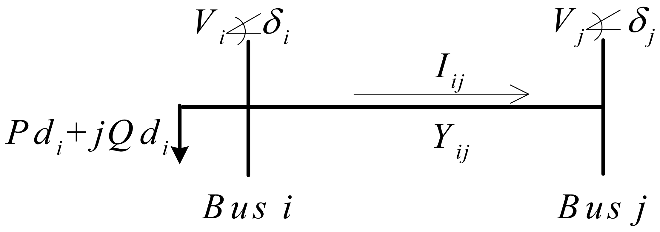
2. Problem Formulation

This section is devoted to the formulation of the problem of locating and sizing DGs. This process is first addressed by defining the objective function, then the set of restrictions associated to the problem are discussed.

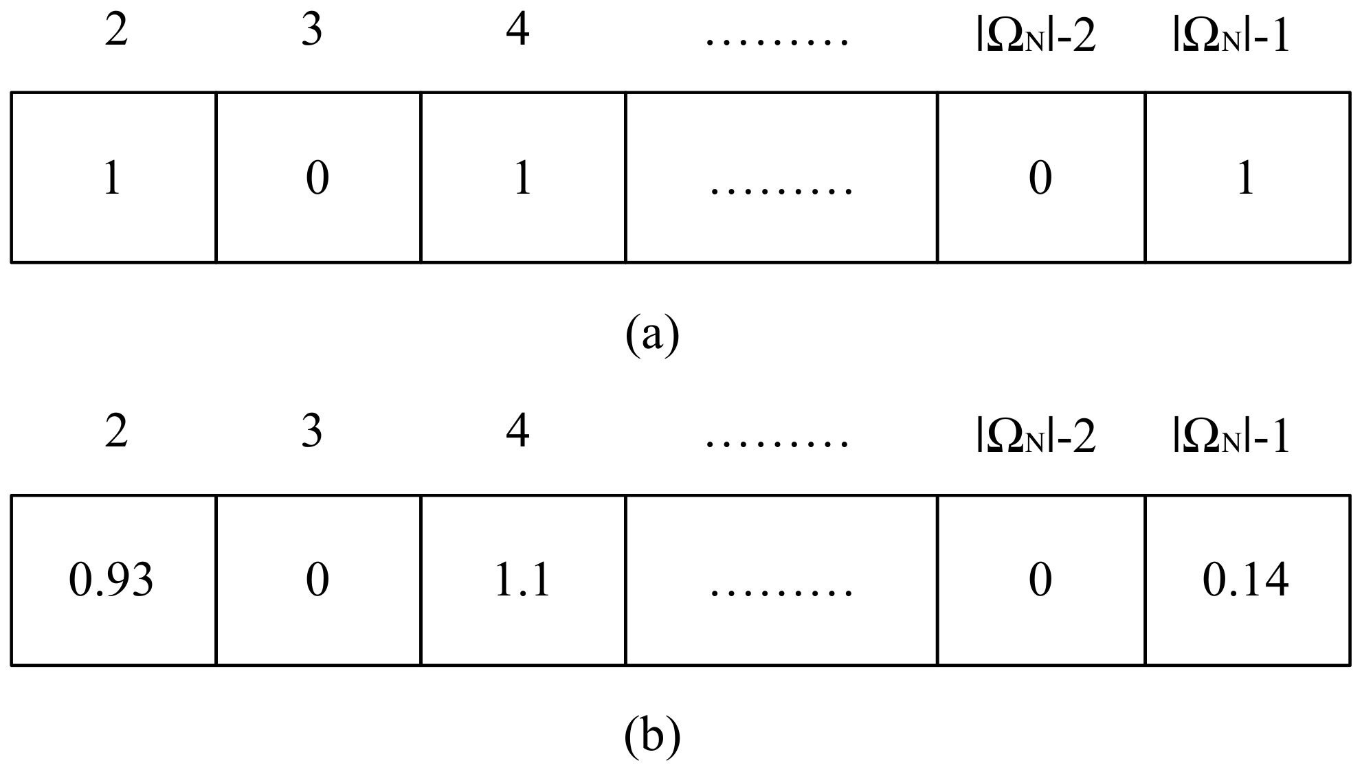
2.1. Optimal Location and Sizing of DGs

The problem is formulated with a weighted single-objective function that combines the objectives of reducing active power losses and improving the voltage profiles by reducing the voltage square error, along with a penalty for limiting the maximum level of penetration of the DGs into the DS. Those criteria were selected on the basis of classic operating restrictions of distribution grids (power balance and operating limits) [20].

The adopted single-objective function is a standard representation commonly used to improve the two principal technical aspects of the electrical power systems [16,20,21,25], the only difference being the limitation of the DGs penetration. Therefore, this type of objective-function is in agreement with the approaches traditionally used for the locating and sizing of DGs in DS [39,40], which enables a fair comparison with other published solutions.

The objective function Z to be minimized in this application is presented in Equation (1), which depends on two weights $(w1,w2)$ used to normalize the functions $f_1$ and $f_2$ at the same units of the active power injection limit ($Pe{n}_{Gen}$).

$$Z=w_1{f}_1+w_2{f}_2+Pe{n}_{Gen}$$

(1)

The function $f_1$ represents the active power losses in the DS (2), while the function $f_2$ is the square error in the voltage profiles of the system in Equation (3). In those expressions $V_i$ and $V_j$ denote the bus voltages at nodes i and j, $V_{base}$ represents the base voltage of the system, ${\theta }_{ij}$ is the angle between voltages $V_i$ and $V_j$, $g_{ij}$ is the conductance between nodes i and j, and ${\mathsf{\Omega }}_B$ is the set of all the branches of the system [41].

$$f_1={\displaystyle \sum _{ij\in {\mathsf{\Omega }}_B}}({V_i}^2+{V_j}^2-2V_i{V}_{j}Cos({\theta }_{ij}))g_{ij}$$

(2)

$$f_2={\displaystyle \sum _{i\in {\mathsf{\Omega }}_{\mathrm{N}}}^n}{(V_i-V_{base})}^2$$

(3)

Finally, Equation (4) presents the expression used to define $Pe{n}_{Gen}$, which affects the objective function when the DGs maximum penetration limit is violated. In expression (4), $P{g}_i$ represents the power generated at bus i by the DGs, $P{g}^{Max}$ is the maximum level of active power allowed to be injected into the system by the DGs, and $F{S}_{Gen}$ is a normalization factor for the penalty.

$$Pe{n}_{Gen}=\left(\left({\displaystyle \sum _{i\in {\mathsf{\Omega }}_N}}P{g}_i\right)-P{g}^{Max}\right)\times F{S}_{Gen}$$

(4)

2.2. Constraints

In order to define the set of restrictions, all the parameters in the system are presented in Figure 1. The diagram represents the DS composed of the output $(i)$ and input $(j)$ buses, the parameters of the line $(R_{ij},X_{ij})$ and a load assigned to the input bus $(j)$.

The set of constraints is presented by Equations (5) to (9). The constraints (5) and (6) represent the bus balance of active and reactive power in the system, respectively. In such expressions $Q{g}_i$ is the reactive power injected into bus i, $P{d}_i$ and $Q{d}_i$ are the active and reactive power demanded at bus i, ${\delta }_i$ and ${\delta }_j$ represent the voltage angles at buses i and j, and $Y_{ij}$ is the admittance of the line $ij$.

$$P{g}_i-P{d}_i-V_i{\displaystyle \sum _{j\in {\mathsf{\Omega }}_N}^{}}{V}_j{Y}_{ij}cos({\delta }_i-{\delta }_j+{\theta }_{ij})=0\forall i\in {\mathsf{\Omega }}_N$$

(5)

$$Q{g}_i-Q{d}_i-V_i{\displaystyle \sum _{j\in {\mathsf{\Omega }}_N}^{}}{V}_j{Y}_{ij}sin({\delta }_i-{\delta }_j+{\theta }_{ij})=0\forall i\in {\mathsf{\Omega }}_N$$

(6)

Equations (7) and (8) represent the limits of bus voltage and current capacity of the system feeders. In those equations ${V_i}^{max}$ and ${V_i}^{min}$ are the maximum and minimum limits of the nodal voltage in the system, $i_{ij}$ is the current of the line $ij$, and $i_{ij}^{max}$ is the maximum current limit allowed in that line.

$${V_i}^{min}\le V_i\le {V_i}^{max}\forall i\in {\mathsf{\Omega }}_N$$

(7)

$$\left|i_{ij}\right|\le {i_{ij}}^{max}\forall i\in {\mathsf{\Omega }}_N$$

(8)

Finally, the restriction (9) models the capacity limits of the DGs. Such a restriction enables the solution of the model without considering generators outside of those ranges. In expression (9), ${P{g}_i}^{max}$ and ${P{g}_i}^{min}$ correspond to the maximum and minimum limits of active power injection allowed for the DGs, which constrain the injection levels (penetration) of the DGs.

$$P{g_i}^{min}\le P{g}_i\le P{g_i}^{max}\forall i\in {\mathsf{\Omega }}_N$$

(9)

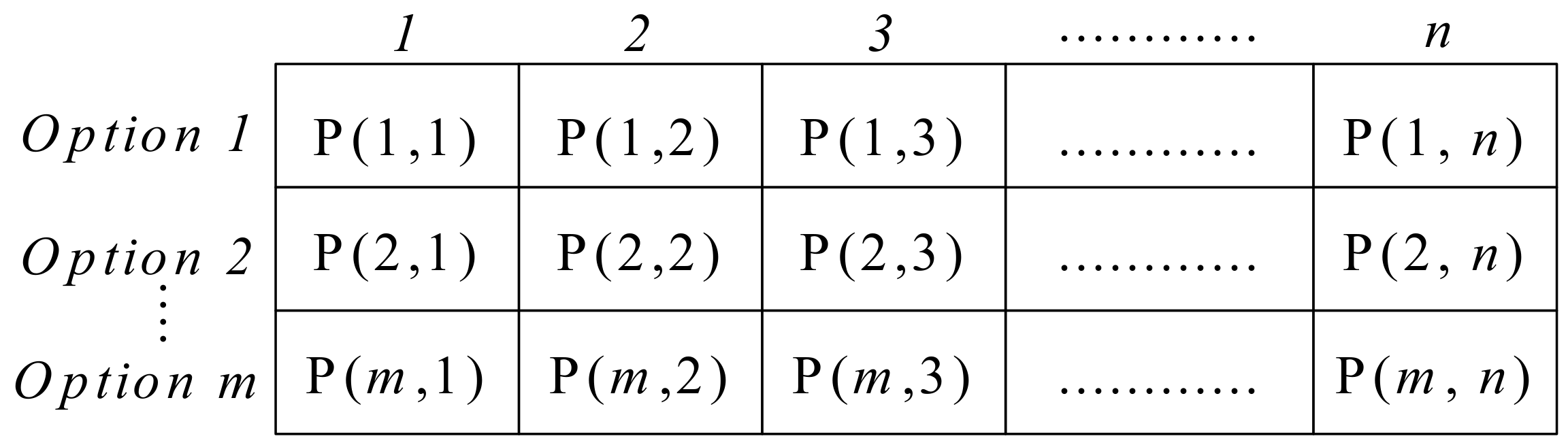
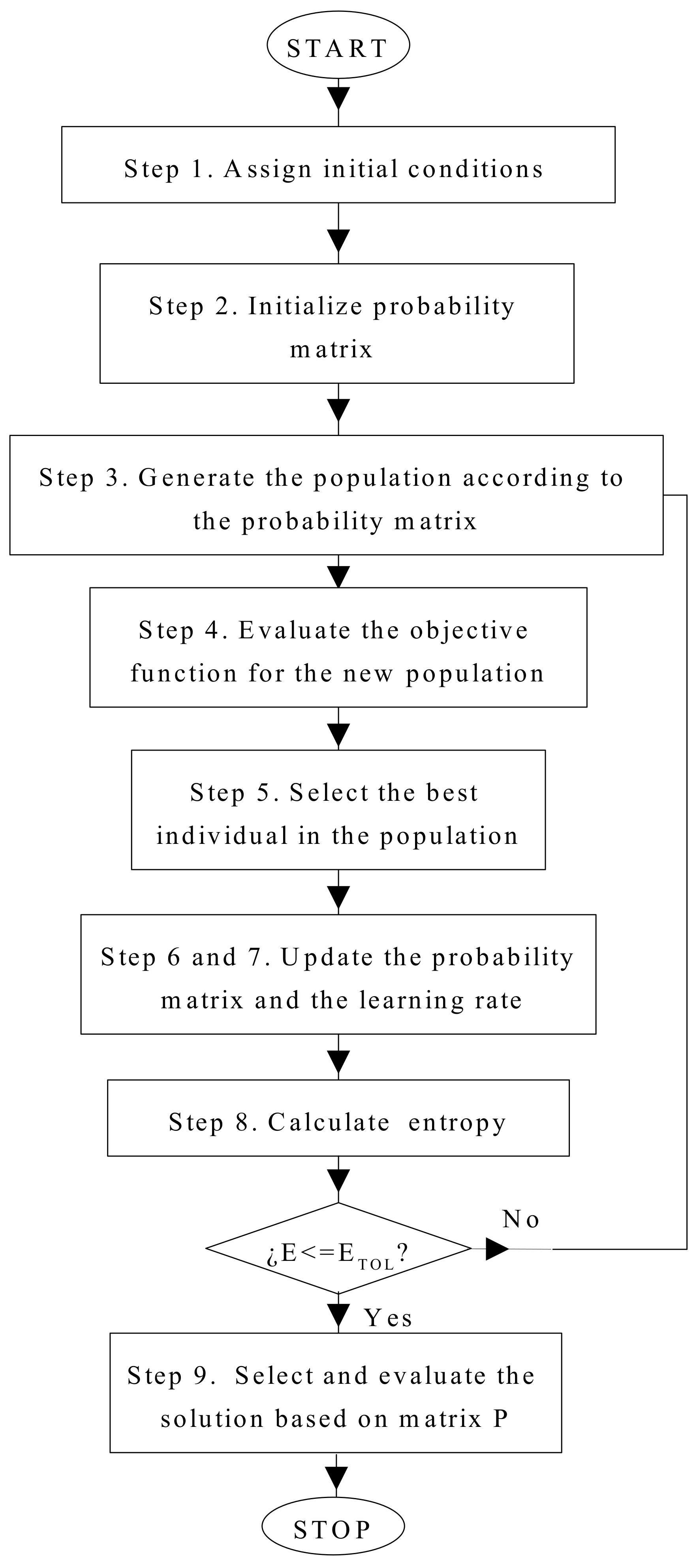
3. Overview of Population-Based Incremental Learning (PBIL)

The PBIL algorithm [28] belongs to the family of EDAs, which have been successfully applied to combinatorial optimization problems [42,43,44], which is the type of problem this paper is facing. Instead of using the classic genetic operators, the EDAs implement automatic learning techniques to estimate a probability distribution associated with the best solution presented by the population, and such a probabilistic model is used to create new candidate solutions [45]. Moreover, the control of the learning rate in each iteration enable to modify the size of the solution space to be explored affecting the processing time [46].

This optimization technique is based on a matrix arrangement that represents all the solution space and stores the probabilities of occurrence of the best solutions to the problem. Such a matrix, known as probability matrix $(P)$, is used to generate the population of individuals, from which the best option should be selected by the objective function. Subsequently, P is updated at each iteration. The main feature of the PBIL algorithm concerns the ability to control the solution space and convergence times by manipulating the learning rate $(LR)$ and the stopping criterion [47]. According to the requirements of the problem, it is possible to select the type (linear, exponential, sigmoidal and bell-shaped) and the maximum and minimum limits of the $LR$. As stopping criterion, the PBIL algorithm adopts the entropy $(E)$, which is responsible for indicating how disperse the data in the probability matrix are. The entropy can be selected to expand the search space, since a small tolerance value forces the algorithm to extend its exploration. The following is a simple and practical way of implementing the PBIL algorithm:

Step 1. Assign initial conditions: First, the algorithm is set with the initial conditions to carry out the iterative process. The following is a description of each condition.

• Population size $(N)$: Number of individuals generated at each iterative cycle of the algorithm. This number depends on the size of the solution space and the desired evaluation spectrum. Then, the initial population is randomly constructed.
• Initial probability: Provides the probability matrix for the initial parameters. In this step the same probability $1/m$ is assigned to each element to be considered in the solution of the problem, providing in this way a fair initial condition. For the binary case discussed here, the initial probability is 0.5 since there are only two options (locate or not a generator in the node).
• Learning rate $(LR)$ type and maximum-minimum limits: $LR$ can be defined in multiple forms, e.g., linear, exponential, sigmoidal and bell-shaped. The assignment of minimum and maximum limits in the range (0–1) enable to control the convergence time and the size of the solution space to be explored [47].
• Stopping criterion $(E_{TOL})$: Defines the stopping condition of the algorithm. For this purpose, an assigned entropy tolerance is in charge of ending the iterative process, i.e., when the entropy reaches that value the algorithm stops. The search intensity of the algorithm depends on the selection of this tolerance; a small tolerance will result in a wider exploration of the solution space.

Step 2. Initialize the probability matrix $(P)$: To construct the probability matrix, the total number of elements to be considered in the solution defines the number of columns $(n)$ of P, as it is depicted in Figure 2. The number of rows of P corresponds to the number of options $(m)$ available for each element. Therefore, each element of P represents the probability of selecting a given option (row) for each element (column). For a binary case there are only two options $(m=2)$, hence each element could be considered, or not, to be present into the problem solution. Instead, for a problem in which more options are available for each individual the value of m will be different [34].

At the beginning of the iterative process, all the probabilities are set to the same value $(1/m)$ to enable the exploration of the complete solution space. Moreover, the probability matrix must to satisfy constraint of Equation (10), in which $P_{(j,k)}$ is the probability of the option j to be selected for the element h. Therefore, the expression (10) ensures that the sum of all the probabilities of a given option is equal to 1, i.e., avoiding an accumulative probability higher that 100 %.

$${\displaystyle \sum _{j=1}^m}{P}_{\left(j,h\right)}=1\forall 1\le h\le n$$

(10)

Step 3. Generate the population according to the probability matrix: At each iteration of the algorithm, a new population of N individuals is generated based on the information stored in matrix P. The goal is to create a new population that incorporates the probability of each option into each element of the solution.

Step 4. Evaluate the objective function for the new population: Each individual in the population is evaluated using the objective function of the problem, storing the resulting value in a vector of N size. Such a vector is used to compare the optimality of the individuals.

Step 5. Select the best individual in the population: Based on the comparison of objective function values for all the individuals in the population, the fittest individual presenting the most appropriate solution is selected. The lowest value is selected when a minimization problem is being addressed; in the case of a maximization problem, it is selected the highest one.

Step 6. Update the probability matrix based on the knowledge about the best individual and learning rate: Based on the information provided by the selected solution, the P values are updated. This increases the probability of occurrence of the element presented in the selected solution and, consequently, reduces the probability of the other possible solutions [34,47]. The latter is achieved by applying the updating processes described by Equations (11) and (12) to the probability matrix.

$${P_{\left(i,j\right)}}_{Act}={P_{\left(i,j\right)}}_{Old}+\left(1-{P_{\left(i,j\right)}}_{Old}\right)\times LR$$

(11)

$${P_{\left(i,j\right)}}_{New}=\left\{\begin{array}{cc}{P_{\left(i,j\right)}}_{Act}& ifi=k\\ \left(1-{P_{\left(i,j\right)}}_{Act}\right)\times \frac{{P_{\left(i,j\right)}}_{Old}}{1-{P_{\left(i,j\right)}}_{Old}}& ifi\ne k\end{array}\right.$$

(12)

In the previous equations $P_{{(i,j)}_{Act}}$ is the update of the probability of position $(i,j)$; $P_{{(i,j)}_{New}}$ is the new value of the probability at position $(i,j)$; and $P_{{(i,j)}_{Old}}$ is the non-updated probability of position $(i,j)$. The index k refers to the option associated with the best solution found for the element j. As a result, the probability associated with row k increases and the probabilities of the other rows decrease, thus maintaining the ratio given in Equation (10). The size of the probabilities incremented in P depends on factor $LR$, which is updated at each iteration, thus enabling control of the convergence rate of the PBIL algorithm.

Step 7. Calculate the learning rate $(LR)$: The type and limits of the learning rate were selected in Step 1. The calculation of the learning rate depends on the established limits and the entropy of the probability matrix, as shown in Equation (13), which is a suitable function introduced in [47]. The selection of the limits depends on the convergence and desired computation times of the algorithm, since it affects the updating of the probability matrix as previously reported in Equation (11).

$$LR=L{R}_{max}-\frac{L{R}_{max}-L{R}_{min}}{1+e^{-10\times \left(E_n-0.5\right)}}$$

(13)

Step 8. Calculate entropy $(E)$: This is a measure of how distributed the values of P are, and it must be updated at each iteration of the algorithm. The maximum value of E is 1, which indicates that the probabilities in P are completely disperse; the minimum value of E is 0, which indicates that the probability matrix converges to an optimal solution. Equation (14) describes the mathematical formulation to calculate the entropy, which has been normalized to obtain the previously described range [47]. $E<E_{TOL}$ was implemented as the stopping criterion of the iterative process of the PBIL algorithm.

$$E=\frac{-{\displaystyle \sum _{i=1}^m}{\displaystyle \sum _{j=1}^{n-1}}{P}_{\left(i,j\right)}\times log\left[P_{\left(i,j\right)}\right]}{n}$$

(14)

Steps 9. Select and evaluate the solution based on matrix P: When the PBIL algorithm converges, it provides the probability matrix with the information about the solution exhibiting the best conditions. Hence, the best solution is obtained by means of the selection and evaluation of the individual based on P.

Finally, Figure 3 presents the flowchart of the PBIL algorithm, which illustrates the iterative process and each step of the algorithm.

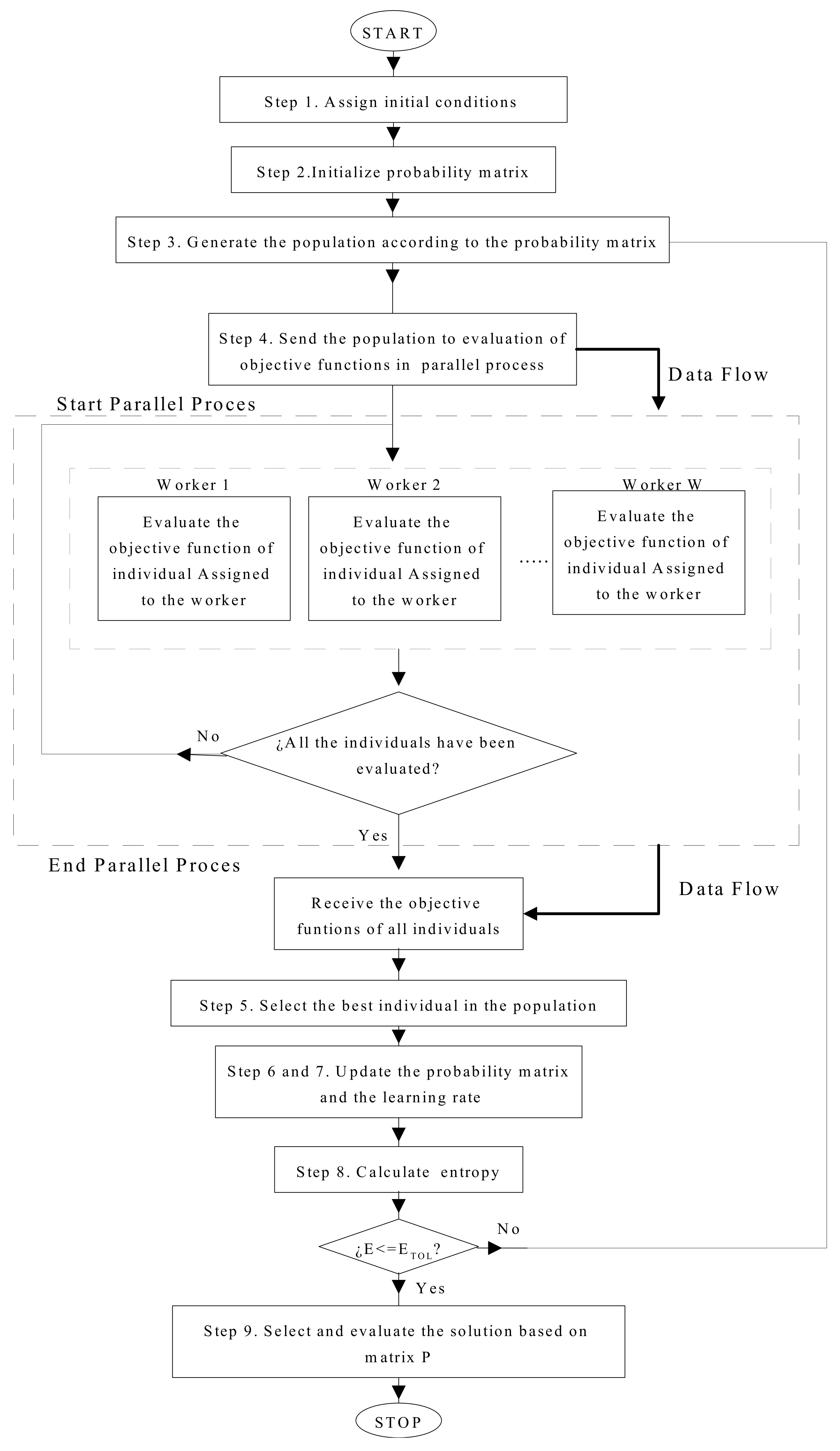
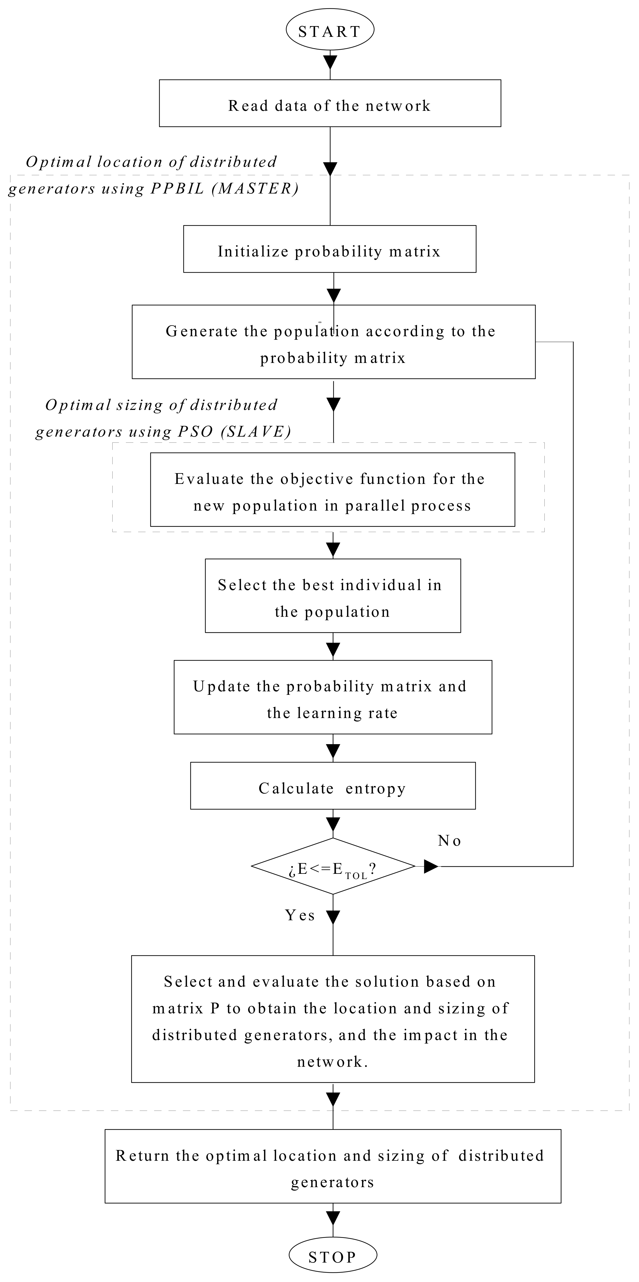
4. Parallel PBIL Algorithm (PPBIL)

Nowadays, engineers must to take advantage of the processors and graphics cards parallel capability to extract the higher value possible from those devices [48,49]. Moreover, parallel processing devices also enable us to significantly decrease the calculation time needed by optimization techniques, such as the PBIL algorithm. The parallelization of the PBIL algorithm takes place in the evaluation of each individual of the population, i.e., Step 4 of the PBIL algorithm. Such a step was selected since that is the stage requiring higher computational effort. Moreover, the variation of the population size depends on the problem being solved, thus enabling evaluation of different individuals in parallel will shorten the computation time with respect to the serial PBIL implementation.

The parallelization limit is defined by the number of workers $(W)$ available in the processor. This is why, when the number of individuals of the population $(N)$ is selected, the equipment to be used should be carefully analyzed, so that the number of individuals is not higher than the number of workers. Otherwise, the computation times would increase, approximately, the number of times such a value is exceeded. When each individual is analyzed by a worker, as a result, the population is analyzed in groups of up to W. In addition, the number of iterations $(B)$ for evaluating all the individuals of the population is calculated as $B=N/W$. Therefore, with the use of parallel processing, the number of iterations to evaluate the population is significantly reduced in comparison with the traditional (serial) implementation. The flowchart presented in Figure 4 shows the PPBIL algorithm, in which the parallelization only affects the evaluation of the objective function of different individuals in the population, the rest of the algorithm is the same of the serial PBIL.

5. Sizing and Location of DGs Using PPBIL-PSO

In order to develop the strategy for optimal location and sizing of DGs, the mathematical model described in Section 2 is solved. This is achieved by adopting a master-slave approach between the PPBIL and PSO algorithms as it is illustrated in Figure 5. For this application the PPBIL is assigned in the master role, locating the generators, and the PSO algorithm [50] is the slave responsible for sizing the generators and evaluating the objective function of the individuals in the population. Such a PSO function was selected due to the satisfactory results reported in literature concerning the sizing of DGs [8,20,22,36].

Both stages use a vector of $(|{\mathsf{\Omega }}_N|-1)$ elements for their codification, except for the Slack node, which is always occupied by the main generator of the grid. Moreover, a binary codification is used for the location: if a position of the vector has a 1, it means that the associated generator is proposed for installation, otherwise, it has a 0 (no installation of the generator). Figure 6 presents an example of such a codification, in which generators are installed at buses 2, 4 and $(|{\mathsf{\Omega }}_N|-1)$. In order to size the DGs, it is necessary to propose a continuous codification that enables to assign the power values to be injected by each generator. Such values should be within the allowed ranges of generation for each DG (maximum and minimum values). Figure 6 presents an example of the sizing codification, in which the maximum power allowed to be injected by the generators is 1.1 MW (assigned to bus 4) and the minimum is 0 MW (assigned to buses 3 and $(|{\mathsf{\Omega }}_N|-2)$).

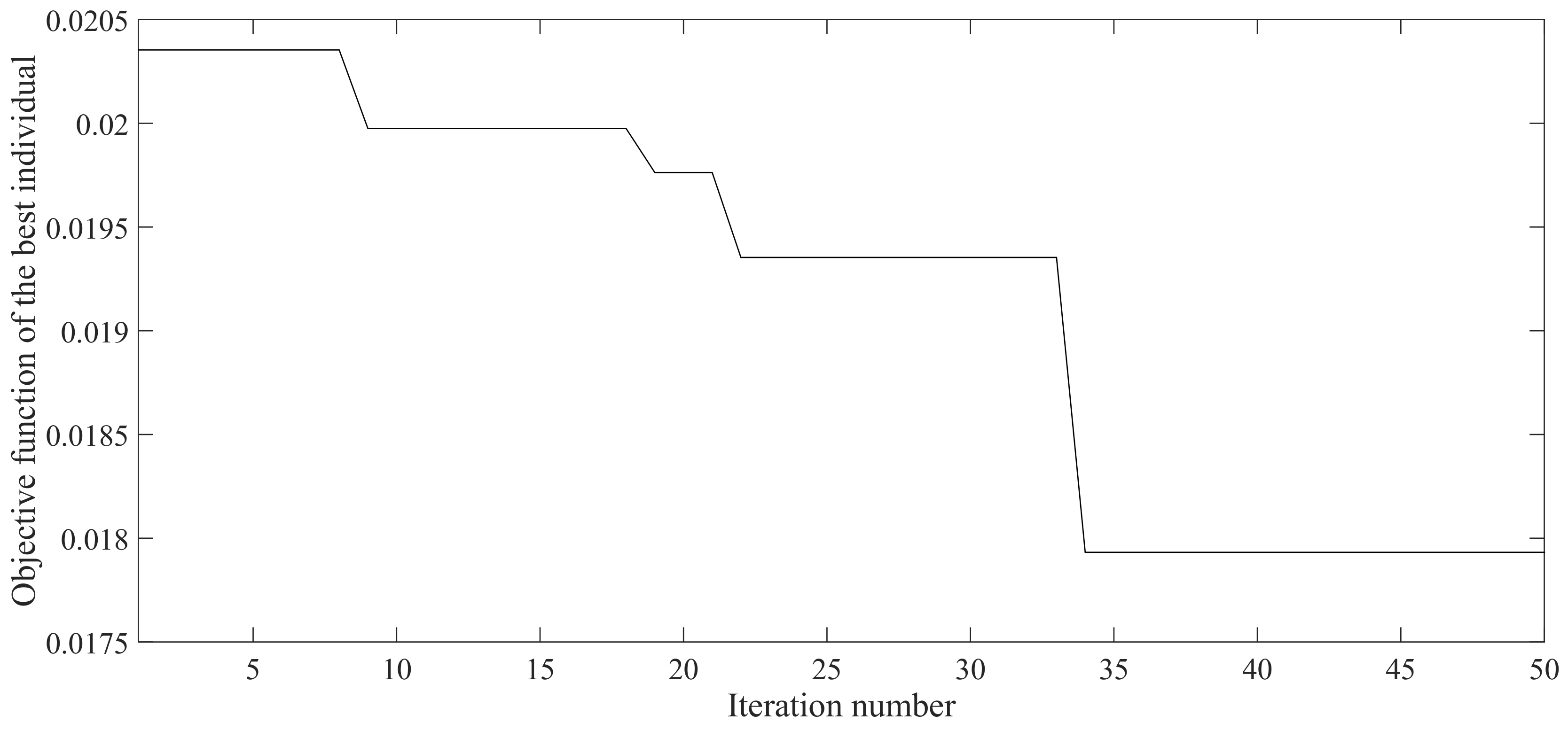
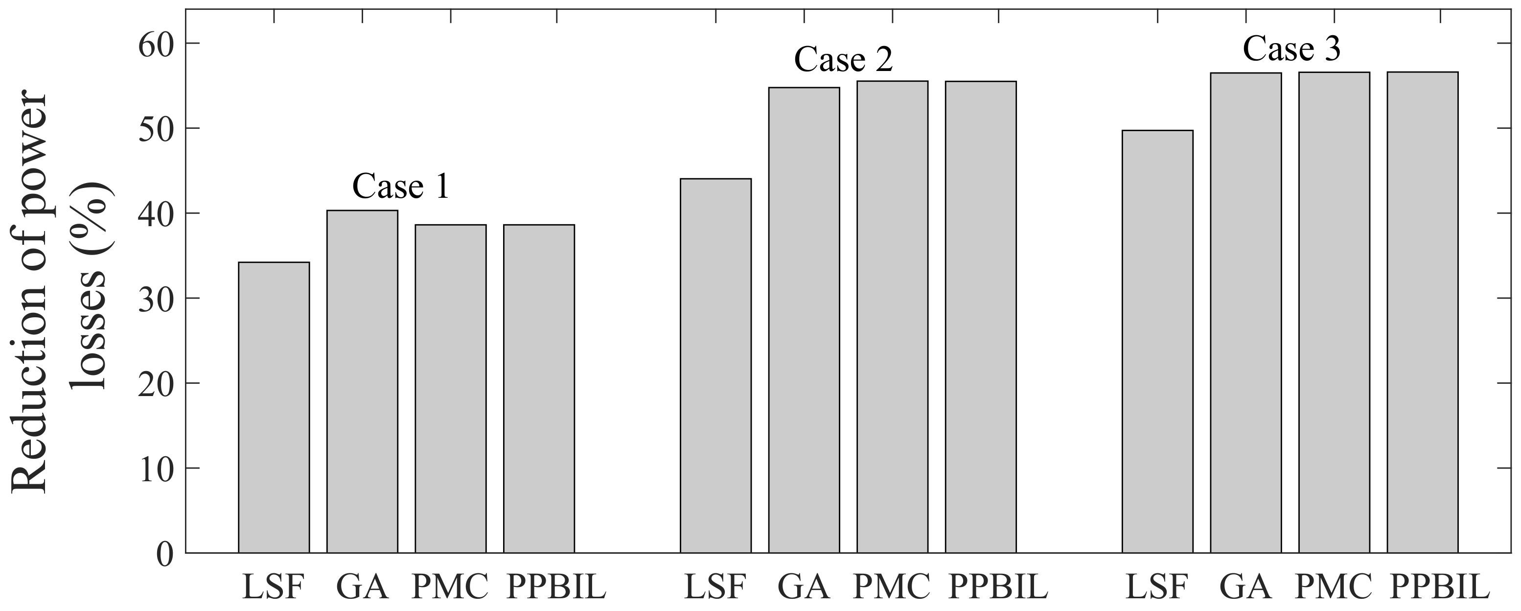
6. Performance Evaluation and Practical Tests

To evaluate the performance of the proposed solution, test systems with 33 and 69 buses were implemented [51] due to their widespread use as benchmarks for this problem [4,8,21,24,25]. Those test systems exhibit high power losses levels and square error in the voltage profiles, providing two different sizes for the solution space. Is worth noting that the test system with 69 buses was derived from a portion of the Pacific Gas and Electric Company’s (PG&E) distribution system based in California (USA) [52], hence it is considered as a mono-phase equivalent circuit of a real system.

In those test systems, all the buses, except for the Slack node, were considered as candidates for DGs installation. Therefore, the probability matrix of the PPBIL algorithm used for locating the DGs has two options: Option 1 indicates that a generator will be installed in the corresponding node, while Option 2 indicates that the generator will not be installed in that node. Besides, the maximum and minimum injection power limits for each generator were defined as 0 W and 1.2 MW, respectively. Such values are selected following the case analyzed in [20], however those limits depend on the application and power system under study [53].

The mathematical model described in Section 2 was implemented for both 33 and 69 bus systems. In both test systems the aim is to reduce active power losses and voltage square error, also constraining the level of penetration of the DGs. The weighting factors of the objective function (1) used for both systems were $(w1=0.1461)$ and $(w2=0.2052)$, which have been tuned by successive iterations of the method. Moreover, three test scenarios were implemented for each test system: the installation of 1, 2 and 3 DGs. In all cases, the maximum penetration allowed for distributed generation was 40% of the power injected by the Slack node under non-distributed generation conditions. This limit was set to control the level of penetration following the recommendation given in [54]. Therefore, the main generator is always present at the Slack node.

To illustrate the effectiveness of the proposed method, a comparison was made with three different strategies traditionally used to locate DGs. The first location strategy is the Loss Sensitive Factor (LSF) [21], which is a heuristic technique based on determining the most sensitive buses in the system suitable to install the DGs. It starts with the bus that presents the worse scenario. Then, in the descending order, it selects from this list the total number of generators to be installed. This method presents relatively short computation times, but it can be trapped into a local optima. Finally, it is worth noting that this method does not use any exhaustive or evolutionary process to move forward. The second technique used for comparison purposes is the Genetic Algorithm (GA) [20], which is a population-based metaheuristic method that allows for a quality solution by means of a process of selection, recombination and mutation of the individuals [55,56,57]. The third strategy is the Monte-Carlo method [38], which is a non-deterministic algorithm aimed at solving computational problems using repeated random sampling of possible solutions. Those solutions are statistically analyzed to determine the one with higher rate occurrence. In this algorithm the error decreases almost proportionally to the number of iterations selected for the implementation. The work reported in [38] describes a PMC algorithm designed to locate and size DGs, with the aims of reducing the power losses and providing short computation times.

The four location approaches (LSF, GA, PMC and PPBIL) are supported by the same PSO for the DGs sizing process. This strategy enables a fair comparison between those location techniques. The parameters of the GA, PMC and PPBIL location algorithms are listed in

Table 1. Parameters of location techniques.

Method	Population Size	Selection Method	Rate Learning	Mutation	Stopping Criterion
GA	12	Tournament	Cross over: simple	Binary simple	Maximum generational cycles (40)
PMC	12	Repeated random sampling	- - - - - - - -	- - - - - - - -	Maximum iterations (10)
PPBIL	12	Initial probability: 0.5	Sigmoidal LRmin: 0.25, LRmax: 0.50	Random Population	Entropy: (0.1)

, while the parameters of the PSO sizing algorithm are listed in

Table 2. Parameters of the sizing technique.

Method	Population Size	Selection Method	Rate Learning	Mutation	Stopping Criterion
PSO	30	Congnitive and social component: 1.4	Speed (Max-Min) (0.1–0.1) Inertia (Max-Min) (0.7–0.001)	R1 = R2: Random	Maximum iterations: (200)

. It is worth noting that LSF is a sensitivity indicator, hence it does not require initial conditions and optimization parameters as reported in [21,25].

The characteristics of the DGs sizing problem changes for every individual generated by the location algorithms, hence the stopping criterion and the size of the population of particles of the PSO algorithm were tuned by successive iterations: the GA/PSO, PMC/PSO and PBIL/PSO were consecutively executed, modifying the maximum number of iterations of the PSO into the range of (0–1000) and the size of population into (20–50). The best convergence rate was achieved for a population size of 30 particles and a maximum number of iterations equal to 200 for all cases as it is reported in Table 2.

The values of the stopping criterion for the GA and PBIL algorithms were obtained by evaluating 100 times each optimization technique. This process was performed using the 69 bus system because it exhibits a larger solution space. Figure 7 reports the averaged number of iterations needed to reach eight different values of entropy within the range of (0.025–0.2) in steps of 0.025: points A, B, C and D corresponds to the objective function of the best individual. Point A is generated by the entropy values 0.200, 0.175 and 0.150; point B is generated by the entropy values 0.0125 and 0.100; point C is generated by the entropy values 0.075 and 0.050; and point D is generated by the entropy value 0.025. Points C and D show that reducing the entropy does not necessarily produce a reduction of the objective function value. Therefore, point B provides a satisfactory trade-off between the objective function value and the number of iterations. Then, the entropy value select for this application is 0.100.

Figure 8 reports the average number of iterations and objective function values obtained after running the GA 100 times. Those results put into evidence that generational cycles higher than 34 do not improve the objective function value. Therefore, the stopping criterion for the GA was fixed at 40 generational cycles.

To provide a fair comparison between the PPBIL and the PMC, the maximum number of iterations for both parallel algorithms must be the same. Hence, the stopping criteria of the PMC was set equal to 10 iterations as reported in Figure 7 (point B). Under the previous considerations, the stopping criteria for the GA, PBIL and PMC are equivalent: all the location algorithms have the opportunity to execute an adequate exploration of the solution space, it taking into account the different nature of the algorithms. Therefore, the parameters given in Table 1 enable a fair comparison between the performance of those location algorithms.

The algorithms were implemented in Matlab (2015a, MathWorks, Natick, MA, USA) using the Matpower tool to evaluate the load flows. The simulations were carried out on a Dell Precision T7600 Worstation that enables to fragment the processor into 12 cores. The simulation results of the test cases for both the 33 and 69 bus systems are summarized in

Table 3. Results of optimal location and sizing of Distributed Generators (DGs) for the test system with 33 buses.

Method	DG Location	DG Size (MW)	Plosses (MW)	%Plosses Reduction	Verror (p.u)	%Verror Reduction	Vworst (p.u)	Processing Time (s)
Without DGs	—–	—–	0.2110	—–	0.1338	—–	0.9037	—–
Case 1: Location of a single DG
LSF	6	1.2	0.1387	34.21	0.0803	39.94	0.9221	31.22
GA	12	1.2	0.1259	40.31	0.0426	68.15	0.9347	639.04
PMC	13	1.2	0.1294	38.62	0.0384	71.28	0.9347	674.79
PPBIL	13	1.2	0.1294	38.62	0.0384	71.28	0.9347	441.34
Case 2: Location of two DGs
LSF	6 28	0.4739 1.0964	0.1180	44.04	0.0598	55.27	0.9277	120.19
GA	16 32	0.7984 0.7719	0.0954	54.77	0.0254	80.99	0.9603	2972.95
PMC	15 30	0.7989 0.7714	0.0938	55.53	0.0275	79.44	0.9552	2073.12
PPBIL	14 32	0.8721 0.6982	0.0938	55.50	0.0258	80.70	0.9590	1654.34
Case 3: Location of three DGs
LSF	6 28 8	0.0001 0.6343 0.9355	0.1060	49.73	0.0472	64.66	0.9400	119.40
GA	14 30 32	0.3203 0.5258 0.2404	0.0917	56.49	0.0276	79.31	0.9572	4075.07
PMC	12 18 31	0.4993 0.3966 0.6744	0.0916	56.57	0.0266	80.08	0.9578	2154.28
PPBIL	12 15 31	0.4035 0.5245 0.6422	0.0915	56.60	0.0265	80.16	0.9570	1794.32

and

Table 4. Results of optimal location and sizing of DGs for the test system with 69 buses.

Method	DG Location	DG Size (MW)	Plosses (MW)	%Plosses Reduction	Verror (p.u)	%Verror Reduction	Vworst (p.u)	Processing Time (s)
Without DGs	—–	—–	0.2421	—–	0.1379	—–	0.9028	—–
Case 1: Location of a single DG
LSF	57	1.2	0.1482	38.79	0.0682	50.52	0.9322	43.35
GA	61	1.2	0.1072	55.70	0.0474	65.61	0.9493	1253.97
PMC	64	1.2	0,1112	54.07	0,0434	68.50	0.9512	953.71
PPBIL	63	1.2	0.1081	55.33	0.0460	66.57	0.9512	696.06
Case 2: Location of two DGs
LSF	57 58	0.4531 1.2	0.1161	52.05	0.0416	69.80	0.9495	165.72
GA	6 62	0.4531 1.2	0.0915	62.20	0.0258	81.26	0.9512	4744.58
PMC	24 63	0.4531 1.2	0.0947	60.85	0.0281	79.57	0.9540	1878.36
PPBIL	61 65	1.2 0.4531	0.0889	63.25	0.0263	80.91	0.9681	1530.75
Case 3: Location of three DGs
LSF	57 58 61	0.0041 0.4490 1.2	0.0914	62.22	0.0308	77.66	0.9620	161.77
GA	53 61 66	0.0001 0.9184 0.7345	0.0872	63.95	0.0247	82.08	0.9681	7511.46
PMC	63 68 69	1.2 0.0577 0.3954	0.0926	61.73	0.0253	81.62	0.9681	2137.64
PPBIL	26 61 66	0.1789 1.0532 0.4209	0.0869	64.07	0.0245	82.89	0.9648	2028.91

. Those tables present the average reduction of both the power losses and voltage error, the average worse bus voltage profile and the average processing time of each technique after 20 executions.

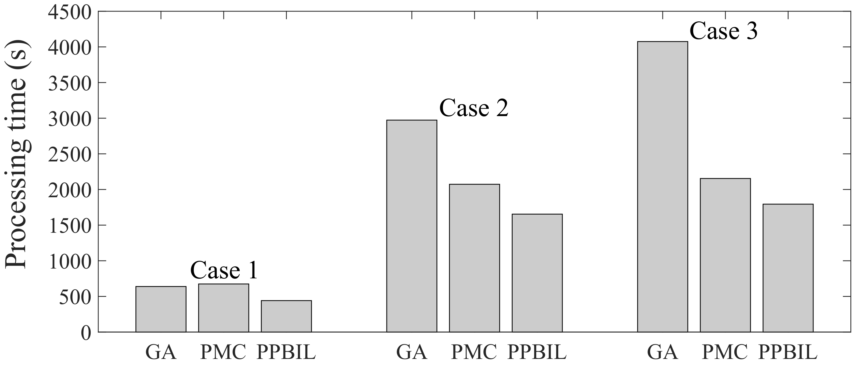
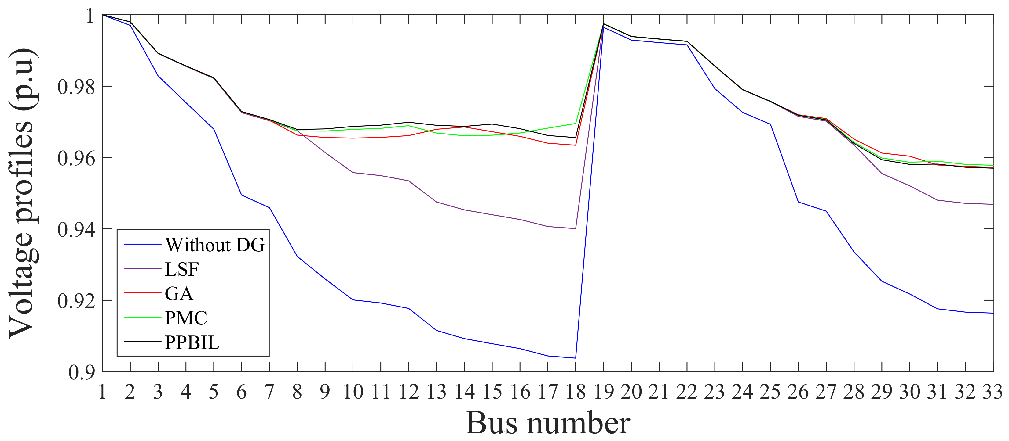
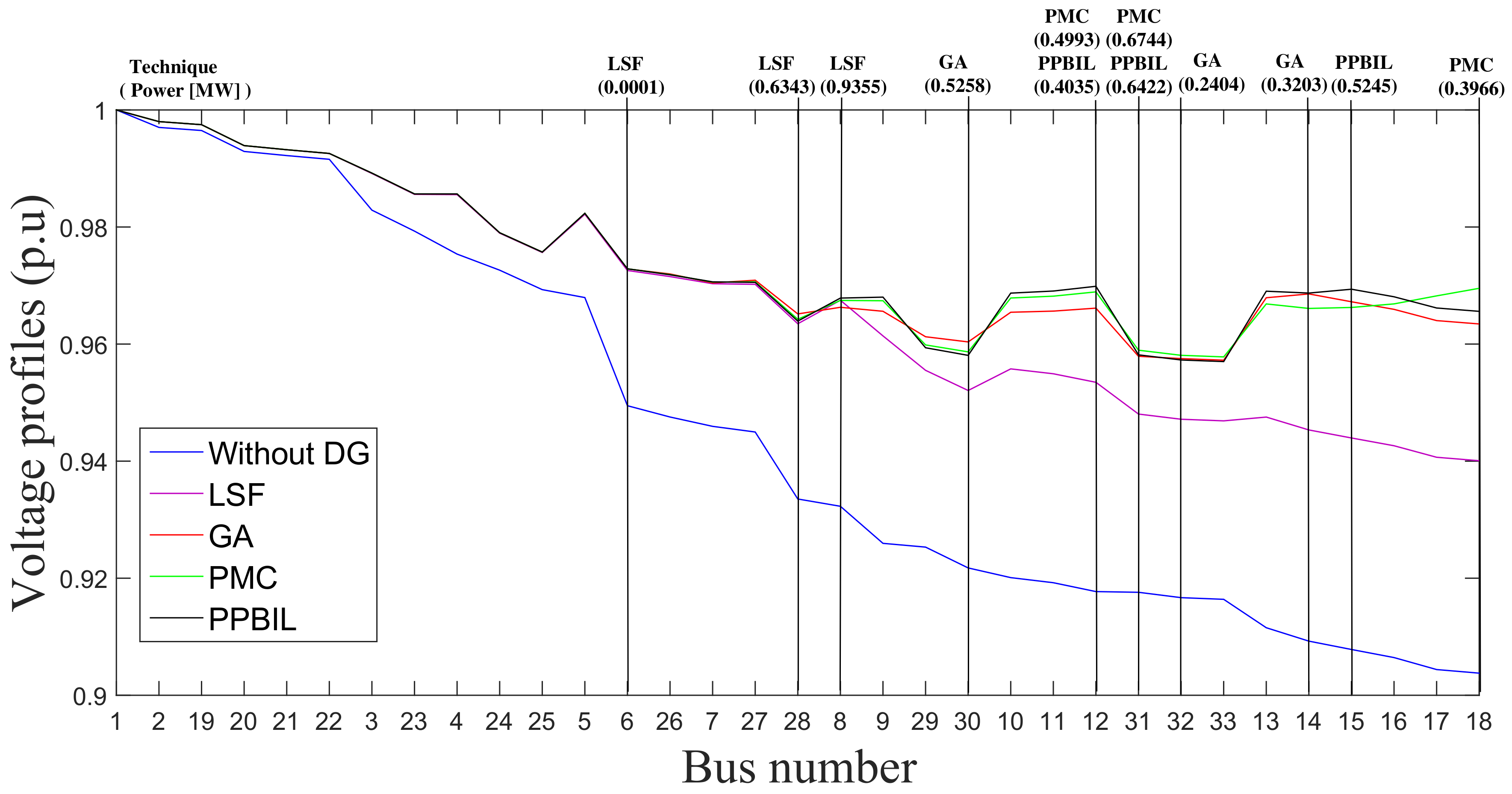
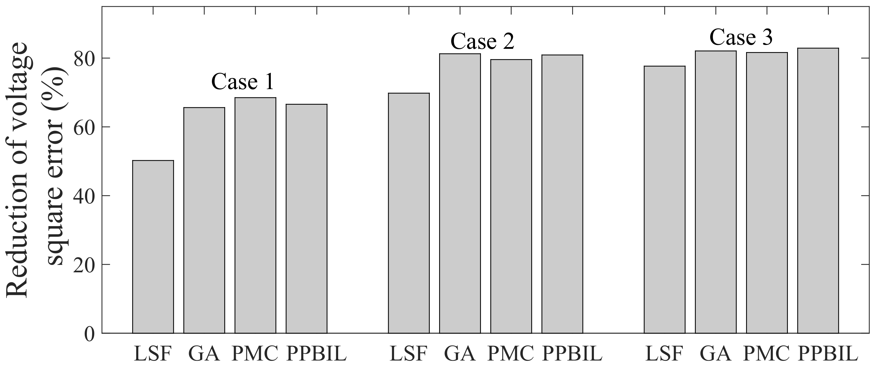
6.1. 33 Bus Test System

This test system is formed by 33 buses and 32 lines. The line diagram of this system is presented in Figure 9, and the data of the line and bus demand were taken from [51]. This system has only one (main) generator with a total active and reactive power demand of 3.72 MW and 2.3 MVAr, respectively, and a voltage level of 12.66 kV. When the initial operating state of the system was analyzed, the power losses were found to be 0.2110 MW and the voltage square error was 0.1338 p.u. Those values were taken as reference to analyze the impact of the integration of DGs using the techniques under test. The detailed information of the branches and power demanded by the buses for this test system is reported in the Appendix A.1.

Table 3 reports the performance of the methods in the reduction of active power losses and the improvement of voltage profiles for the three cases: installation of one, two or three DGs. For comparison and analysis purposes, Table 3 presents the following information from left to right: adopted method, location of the generators (buses), size of the generators (MW), power losses (MW), reduction of active power losses compared to the reference case (Without DGs), voltage square error (p.u.), reduction of the voltage square error compared to the reference case, worse bus voltage in the system and, finally, processing time of the algorithm.

Figure 10 shows that PPBIL becomes the best solution as the exploration space grows. For Case 1, The PPBIL algorithm presents a minimum reduction of active power losses equal to 38.62%, which is the same obtained by the PMC, and just 1.69% lower than the best solution (GA). For Case 2, the PPBIL algorithm presents the second best solution, with a reduction of 57.20%, i.e., 0.73% higher than GA and 11.46% above LSF; in this case PMC is the best solution just by 0.03%. For Case 3, the PPBIL provides the best solution, with a reduction of 56.60%, i.e., 0.03% and 0.11% higher than PMC and GA, respectively, and 6.87% above LSF. Finally, it is noted that LSF provides a satisfactory performance for a small solution space, but it is outperformed by the optimization techniques as the solution space grows.

Similarly, Figure 11 illustrates the impact of each method in the reduction of the voltage square error. In all the test cases, LSF produced the lowest impact on the reduction of the voltage square error. The PMC tied with the PPBIL in Case 1 for the best solution, but it is behind PPBIL in cases 2 and 3: in Case 2 PPBIL is superior by 1.26% and in Case 3 PPBIL provides an additional reduction of 0.08%. The GA presents the best solution in Case 2, but it is behind PBIL in cases 1 and 3: in Case 1 PPBIL provides a 3.13% higher reduction, and in Case 2 PPBIL is 0.85% better. Based on the previous results, the PPBIL algorithm provides the best average results in terms of power losses reduction and voltage profile improvement.

The effectiveness of the PPBIL algorithm in reducing the computation time is illustrated in Figure 12, which shows that PPBIL outperforms both PMC and GA in all the testing cases. It is worth noting that a comparison with the LSF technique is not made because it does not contain an iterative convergence process, which would make a comparison with the optimization techniques unfair. The PPBIL presents a reduction in the computation time of: 30.94% with respect to GA and 34.60% with respect to PMC for Case 1, 44.35% with respect to GA and 20.20% with respect to PMC for Case 2, and 55.97% with respect to GA and 16.71% with respect to PMC for Case 3. Therefore, the PPBIL solution provides shorter processing times in all the cases.

The techniques adopted in literature are traditionally aimed to force all the bus profiles to be as close as possible to the nominal voltage (1 p.u.) [4]. Therefore, the PPBIL, PMC, GA and LSF techniques must also comply such an objective. This is illustrated in Figure 13, which presents the voltage profiles for Case 3, where those techniques introduce a positive impact on the voltage profiles. Moreover, the figure also put into evidence that the PPBIL algorithm exhibits the best voltage profiles. It is worth mentioning that Figure 13 is a classical representation of a power system that depicts the voltage profiles of the buses in the order defined by the line diagram of Figure 9. This is the reason of the strong difference between the voltage profiles of buses 18 and 19: bus 19 is much closer to the main generator (Slack node 1), therefore it exhibits a lower voltage error in comparison with bus 18, which is at the end of the line diagram, i.e., it is subjected to larger distribution losses.

The voltage losses in each node depicted in Figure 13 depend on the distance of the bus to the Slack node and on the power transmitted in the path leading to the node. Therefore, two nodes at the same distance could exhibit different voltage losses. To illustrate better the impact of the DGs designed by the solutions under tests, Figure 14 shows the voltage profiles of the test system with the buses ordered from best to worst voltages without accounting for DGs. This means that, for the reference case (without DG), the voltage profiles are always in descending order of voltage values. Hence, buses 19 and 18 are in opposite sides of Figure 14, third position for bus 19 and last position for bus 18.

Figure 14 confirms that buses located far from the Slack node, or in the path of a high power demand (reported in Appendix A.1), exhibit higher voltage losses. Figure 14 also reports the voltage profiles of the system accounting for the DGs designed by the four solutions under test, describing also the buses in which the DGs have been located and the size of each generator. The figure puts into evidence the improvement on the voltage profiles provided by each solution: the LSF is the technique with the worst performance, while both PMC and GA exhibit improvement on the 93.94% of the buses, finally PPBIL provides improvement on the 96.96% of the buses. Both parallel solutions (PPBIL and PMC) outperform GA, where PMC improves 72.72% of the buses voltage with respect to GA, and PPBIL improves 75.75% of the buses voltage also with respect to GA. Finally, PPBIL exhibits the best performance, since such an algorithm improves 66.66% of the buses voltage with respect to PMC.

In conclusion, the PPBIL solution provides the best average voltage profiles, the lowest average power losses and the shorter processing times for this test system.

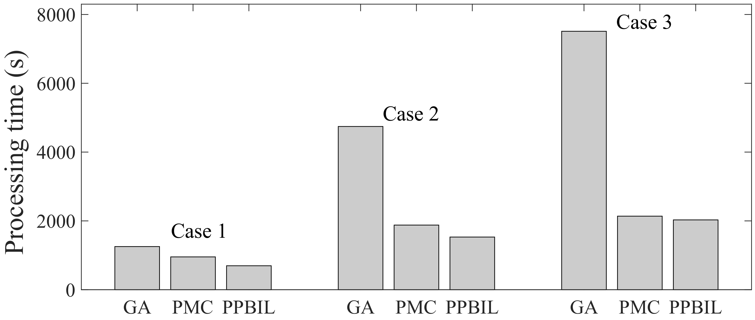
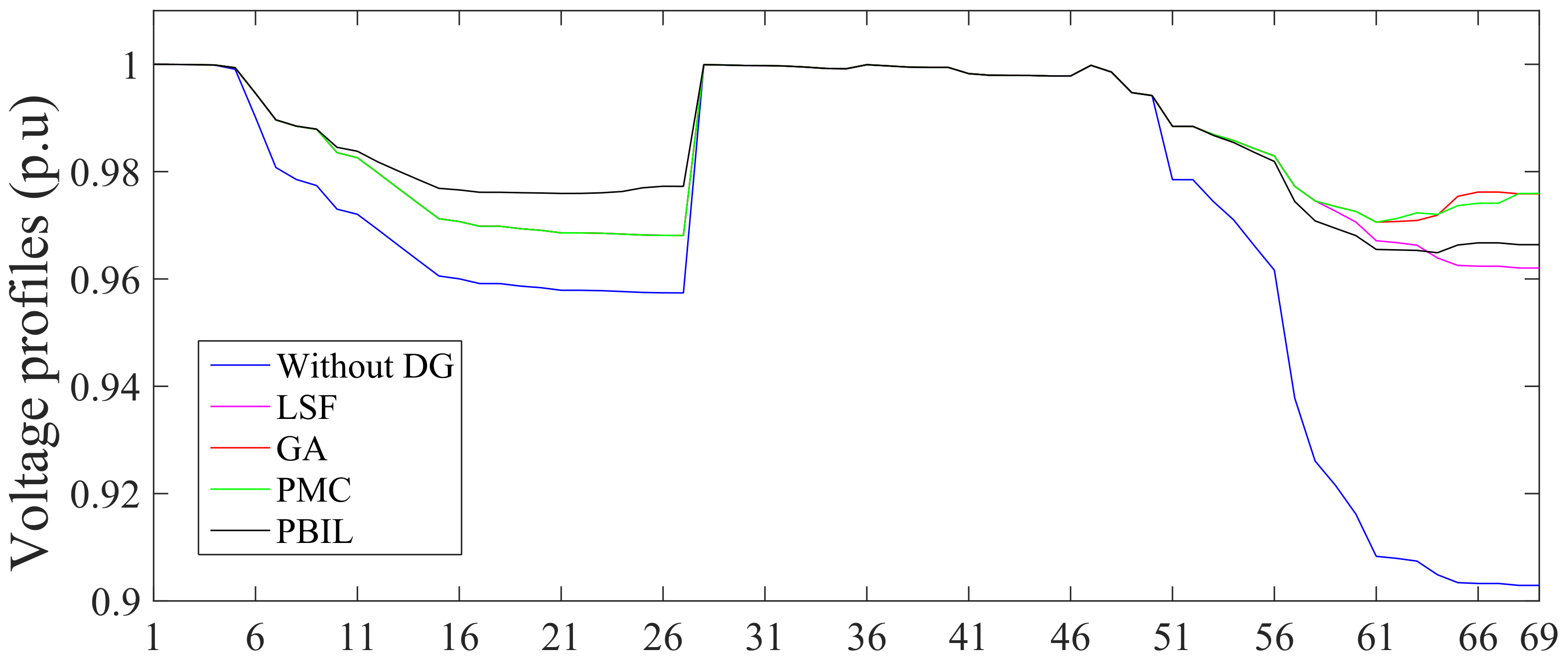
6.2. 69 Bus Test System

This test system is formed by 69 buses and 68 lines following the line diagram presented in Figure 15. The data about the line and bus demand for this example were taken from [51]. This system includes only one generator with a total active and reactive power demand of 3.80 MW and 2.69 MVAr, respectively, and a voltage level of 12.66 kV. The initial operating state of the system was analyzed to find power losses equal to 0.2421 MW and a voltage square error equal to 0.1379 p.u. The detailed information of the branches and power demanded by the buses for this test system is reported in the Appendix A.2. Table 4 summarizes the results of applying all the methods under test to the same three cases: installation of one, two or three DGs.

Figure 16 shows the performance of those techniques in the reduction of power losses. In the figure it is observed that, as the exploration space grows, the PPBIL becomes the best solution: this algorithm presents a minimum reduction of active power losses of 55.33%, just 0.37% less than the best solution for Case 1 (GA). Instead, for both Case 2 and Case 3 the PPBIL solution provides the best global solution, e.g., 2.34% and 0.12% more than PMC and GA in Case 3, respectively. Moreover, PPBIL outperforms LSF in the three cases. Finally, PPBIL is the best solution in terms of averaged power losses reduction.

The impact of each method on the reduction of the voltage square error is illustrated in Figure 17. Again, the PPBIL provides the averaged best performance: its lowest reduction was produced in Case 1 (66.57%), while the highest reduction was produced in Case 3 (82.89%), being the best solution for that case. In Case 2 the PPBIL was outperformed by the PMC in 1.93% and by the GA in 0.35%. Finally, it is worth mentioning that the difference between PPBIL and LSF is noticeable in all cases.

The effectiveness of the PPBIL algorithm in reducing the computation time for the 69 bus test system is illustrated in Figure 18, which makes evident that PPBIL outperforms both PMC and GA in all the cases. In particular, the PPBIL provides a reduction of the computation time in Case 1 equal to 27.02% in comparison with PMC, and equal to 44.49% in comparison with GA. For Case 2, the improvement of the PPBIL is equal to 18.51% (PMC) and 67.74% (GA), and for Case 3 the improvement of the PPBIL is equal to 5.43% (PMC) and 72.99% (GA). Therefore, the proposed PPBIL solution provides the shorter processing times.

Figure 19 presents the voltage profiles for Case 3. As in the previous test system, all the techniques provide a positive impact on the operational aspects of the grid. However, the PPBIL algorithm provides superior voltage profiles for a larger number of buses.

Following the same analysis discussed for the test system with 33 buses, Figure 20 presents the voltage profiles of test system with the 69 buses ordered from best to worst bus voltage without accounting for DGs (reference case). The figure shows that LSF improves the lowest impact on the system voltages, while GA, PMC and PPBIL outperform LSF by 15.94%,15.94% and 82.60% of the buses voltage, respectively. Similarly, the PMC and PPBIL outperform GA in 7.24% y 73.91% of the buses voltage, respectively. Finally, the PPBIL solution improves the voltage profiles in the higher number of buses in comparison with the PMC, 73.91% in this case. In conclusion, the PPBIL algorithm is the one providing the best performance to the system in terms of voltage profiles.

7. Conclusions

This document has presented a parallelization of the PBIL algorithm, named PPBIL, to develop a hybrid PPBIL-PSO method for optimal location and sizing of DGs in electrical systems. The performance of the proposed method was evaluated with two test systems: 33 and 69 buses accounting for the installation of 1, 2 or 3 generators. The new technique was compared with the LSF, GA and PMC solutions, by using the same PSO for the sizing of the four location methods. Such a testing strategy has demonstrated the robustness and efficiency of the method proposed in this paper.

To evaluate the impact of the proposed method, three criteria were analyzed: reduction of active power losses, voltage square error and computation time. The results put into evidence that the PPBIL provides the best balance between processing time, voltage profiles and reduction of power losses in comparison with the PMC, GA and LSF solutions. In particular, the PPBIL provides shorter processing times, which enables to explore large solution spaces within practical times. However, the computation time of the PPBIL algorithm is closely related to the number of workers the processor can be fractionated into. This can be addressed by adopting GPUs as processing units, which allow hundreds of processes in parallel. Such an approach will reduce the convergence time and enable to expand the solution space by increasing the number of individuals in the population, thus making possible to find better solutions to the problem under analysis.

References

1. Huang, Y.; Söder, L. Evaluation of economic regulation in distribution systems with distributed generation. Energy 2017, 126, 192–201. [Google Scholar] [CrossRef]
2. Colmenar-Santos, A.; Reino-Rio, C.; Borge-Diez, D.; Collado-Fernández, E. Distributed generation: A review of factors that can contribute most to achieve a scenario of DG units embedded in the new distribution networks. Renew. Sustain. Energy Rev. 2016, 59, 1130–1148. [Google Scholar] [CrossRef]
3. Ameli, A.; Ahmadifar, A.; Shariatkhah, M.H.; Vakilian, M.; Haghifam, M.R. A dynamic method for feeder reconfiguration and capacitor switching in smart distribution systems. Int. J. Electr. Power Energy Syst. 2017, 85, 200–211. [Google Scholar] [CrossRef]
4. Gopiya Naik, S.; Khatod, D.; Sharma, M. Optimal allocation of combined DG and capacitor for real power loss minimization in distribution networks. Int. J. Electr. Power Energy Syst. 2013, 53, 967–973. [Google Scholar] [CrossRef]
5. Savić, A.; Đurišić, Ž. Optimal sizing and location of SVC devices for improvement of voltage profile in distribution network with dispersed photovoltaic and wind power plants. Appl. Energy 2014, 134, 114–124. [Google Scholar] [CrossRef]
6. De Lima, M.A.X.; Clemente, T.R.N.; de Almeida, A.T. Prioritization for allocation of voltage regulators in electricity distribution systems by using a multicriteria approach based on additive-veto model. Int. J. Electr. Power Energy Syst. 2016, 77, 1–8. [Google Scholar] [CrossRef]
7. Santos, S.F.; Fitiwi, D.Z.; Cruz, M.R.; Cabrita, C.M.; Catalão, J.P. Impacts of optimal energy storage deployment and network reconfiguration on renewable integration level in distribution systems. Appl. Energy 2017, 185, 44–55. [Google Scholar] [CrossRef]
8. Daud, S.; Kadir, A.; Gan, C.; Mohamed, A.; Khatib, T. A comparison of heuristic optimization techniques for optimal placement and sizing of photovoltaic based distributed generation in a distribution system. Sol. Energy 2016, 140, 219–226. [Google Scholar] [CrossRef]
9. Picciariello, A.; Alvehag, K.; Soder, L. State-of-art review on regulation for distributed generation integration in distribution systems. In Proceedings of the 2012 9th International Conference on the European Energy Market, Florence, Italy, 10–12 May 2012; pp. 1–8. [Google Scholar]
10. Minnaar, U. Regulatory practices and Distribution System Cost impact studies for distributed generation: Considerations for South African distribution utilities and regulators. Renew. Sustain. Energy Rev. 2016, 56, 1139–1149. [Google Scholar] [CrossRef]
11. Chiradeja, P.; Ramakumar, R. An Approach to Quantify the Technical Benefits of Distributed Generation. IEEE Trans. Energy Convers. 2004, 19, 764–773. [Google Scholar] [CrossRef]
12. Prakash, P.; Khatod, D.K. Optimal sizing and siting techniques for distributed generation in distribution systems: A review. Renew. Sustain. Energy Rev. 2016, 57, 111–130. [Google Scholar] [CrossRef]
13. Balamurugan, K.; Srinivasan, D.; Reindl, T. Impact of Distributed Generation on Power Distribution Systems. Energy Procedia 2012, 25, 93–100. [Google Scholar] [CrossRef]
14. Rezaee Jordehi, A. Allocation of distributed generation units in electric power systems: A review. Renew. Sustain. Energy Rev. 2016, 56, 893–905. [Google Scholar] [CrossRef]
15. Theo, W.L.; Lim, J.S.; Ho, W.S.; Hashim, H.; Lee, C.T. Review of distributed generation (DG) system planning and optimisation techniques: Comparison of numerical and mathematical modelling methods. Renew. Sustain. Energy Rev. 2017, 67, 531–573. [Google Scholar] [CrossRef]
16. Pesaran, H.A.M.; Huy, P.D.; Ramachandaramurthy, V.K. A review of the optimal allocation of distributed generation: Objectives, constraints, methods, and algorithms. Renew. Sustain. Energy Rev. 2017, 75, 293–312. [Google Scholar] [CrossRef]
17. Ouyang, W.; Cheng, H.; Zhang, X.; Yao, L. Distribution network planning method considering distributed generation for peak cutting. Energy Convers. Manag. 2010, 51, 2394–2401. [Google Scholar] [CrossRef]
18. Chu, P.; Beasley, J. A genetic algorithm for the generalized assignment problem. Comput. Oper. Res. 1997, 24, 17–23. [Google Scholar] [CrossRef]
19. El-Zonkoly, A. Optimal placement of multi-distributed generation units including different load models using particle swarm optimization. Swarm Evol. Comput. 2011, 1, 50–59. [Google Scholar] [CrossRef]
20. Moradi, M.; Abedini, M. A combination of genetic algorithm and particle swarm optimization for optimal DG location and sizing in distribution systems. Int. J. Electr. Power Energy Syst. 2012, 34, 66–74. [Google Scholar] [CrossRef]
21. Mohamed Imran, A.; Kowsalya, M. Optimal size and siting of multiple distributed generators in distribution system using bacterial foraging optimization. Swarm Evol. Comput. 2014, 15, 58–65. [Google Scholar] [CrossRef]
22. Jain, N.; Singh, S.; Srivastava, S. PSO based placement of multiple wind DGs and capacitors utilizing probabilistic load flow model. Swarm Evol. Comput. 2014, 19, 15–24. [Google Scholar] [CrossRef]
23. Kefayat, M.; Lashkar Ara, A.; Nabavi Niaki, S. A hybrid of ant colony optimization and artificial bee colony algorithm for probabilistic optimal placement and sizing of distributed energy resources. Energy Convers. Manag. 2015, 92, 149–161. [Google Scholar] [CrossRef]
24. Saha, S.; Mukherjee, V. Optimal placement and sizing of DGs in RDS using chaos embedded SOS algorithm. IET Gener. Transm. Distrib. 2016, 10, 3671–3680. [Google Scholar] [CrossRef]
25. Ali, E.; Abd Elazim, S.; Abdelaziz, A. Ant Lion Optimization Algorithm for optimal location and sizing of renewable distributed generations. Renew. Energy 2017, 101, 1311–1324. [Google Scholar] [CrossRef]
26. Kaur, S.; Kumbhar, G.B.; Sharma, J. Performance of Mixed Integer Non-linear Programming and Improved Harmony Search for optimal placement of DG units. In Proceedings of the 2014 IEEE PES General Meeting | Conference Exposition, National Harbor, MD, USA, 27–31 July 2014; pp. 1–5. [Google Scholar]
27. Kaur, S.; Kumbhar, G.; Sharma, J. A MINLP technique for optimal placement of multiple DG units in distribution systems. Int. J. Electr. Power Energy Syst. 2014, 63, 609–617. [Google Scholar] [CrossRef]
28. Baluja, S. Population-Based Incremental Learning: A Method for Integrating Genetic Search Based Function Optimization and Competitive Learning; School of Computer Science, Carnegie Mellon University: Pittsburgh, Pennsylvania, 1994; pp. 1–41. [Google Scholar]
29. Wang, J.; Zhou, Y.; Yin, J.; Zhang, Y. Competitive hopfield network combined with estimation of distribution for maximum diversity problems. IEEE Trans. Syst. Man Cybern. B Cybern. 2009, 39, 1048–1066. [Google Scholar] [CrossRef] [PubMed]
30. Xu, Z.; Wang, Y.; Li, S.; Liu, Y.; Todo, Y.; Gao, S. Immune algorithm combined with estimation of distribution for traveling salesman problem. IEEJ Trans. Electr. Electron. Eng. 2016, 11, S142–S154. [Google Scholar] [CrossRef]
31. Rastegar, R. On the Optimal Convergence Probability of Univariate Estimation of Distribution Algorithms. Evol. Comput. 2011, 19, 225–248. [Google Scholar] [CrossRef] [PubMed]
32. Carnero, M.; Hernández, J.; Sánchez, M. A new metaheuristic based approach for the design of sensor networks. Comput. Chem. Eng. 2013, 55, 83–96. [Google Scholar] [CrossRef]
33. Folly, K.A.; Venayagamoorthy, G.K. Power system controller design using multi-population PBIL. In Proceedings of the 2013 IEEE Computational Intelligence Applications in Smart Grid (CIASG), Singapore, 16–19 April 2013; pp. 37–43. [Google Scholar]
34. Bolanos, F.; Aedo, J.E.; Rivera, F.; Bagherzadeh, N. Mapping and Scheduling in Heterogeneous NoC through Population-Based Incremental Learning. J. Univers. Comput. Sci. 2012, 18, 901–916. [Google Scholar]
35. Corea-Araujo, J.A.; Martinez-Velasco, J.A.; Magnusson, J. Optimum design of hybrid HVDC circuit breakers using a parallel genetic algorithm and a MATLAB-EMTP environment. IET Gener. Transm. Distrib. 2017, 11, 2974–2982. [Google Scholar] [CrossRef]
36. Kansal, S.; Kumar, V.; Tyagi, B. Optimal placement of different type of DG sources in distribution networks. Int. J. Electr. Power Energy Syst. 2013, 53, 752–760. [Google Scholar] [CrossRef]
37. Ahmad Khan, A.; Naeem, M.; Iqbal, M.; Qaisar, S.; Anpalagan, A. A compendium of optimization objectives, constraints, tools and algorithms for energy management in microgrids. Renew. Sustain. Energy Rev. 2016, 58, 1664–1683. [Google Scholar] [CrossRef]
38. Martinez, J.A.; Guerra, G. A parallel Monte Carlo method for optimum allocation of distributed generation. IEEE Trans. Power Syst. 2014, 29, 2926–2933. [Google Scholar] [CrossRef]
39. Grisales, L.F.; Restrepo Cuestas, B.J.; Jaramillo, F.E. Ubicación y dimensionamiento de generación distribuida: Una revisíon. Cienc. Ing. Neogranad. 2017, 27, 157–176. [Google Scholar] [CrossRef]
40. Nekooei, K.; Farsangi, M.M.; Nezamabadi-Pour, H.; Lee, K.Y. An Improved Multi-Objective Harmony Search for Optimal Placement of DGs in Distribution Systems. IEEE Trans. Smart Grid 2013, 4, 557–567. [Google Scholar] [CrossRef]
41. Grainger, J.; Stevenson, W. Power System Analysis; McGraw Hill: New York, NY, USA, 1994; p. 743. [Google Scholar]
42. Ceberio, J.; Irurozki, E.; Mendiburu, A.; Lozano, J.A. A review on estimation of distribution algorithms in permutation-based combinatorial optimization problems. Prog. Artif. Intell. 2012, 1, 103–117. [Google Scholar] [CrossRef]
43. Larrañaga, P.; Karshenas, H.; Bielza, C.; Santana, R. A review on probabilistic graphical models in evolutionary computation. J. Heuristics 2012, 18, 795–819. [Google Scholar] [CrossRef] [Green Version]
44. Shakya, S.; Santana, R. A Review of Estimation of Distribution Algorithms and Markov Networks; Chapter 2-A Review; Springer: Berlin, Germany, 2012; pp. 21–37. [Google Scholar]
45. González, C.; Lozano, J.A.; Larrañaga, P. The Convergence Behavior of the PBIL Algorithm: A Preliminary Approach. In Artificial Neural Nets and Genetic Algorithms; Springer: Vienna, Austria, 2001; pp. 228–231. [Google Scholar]
46. Zangari, M.; Santana, R.; Mendiburu, A.; Pozo, A. Not all PBILs are the same: Unveiling the different learning mechanisms of PBIL variants. Appl. Soft Comput. 2017, 53, 88–96. [Google Scholar] [CrossRef]
47. Bolanos, F.; Aedo, J.E.; Rivera, F. Comparison of Learning Rules for Adaptive Population-Based Incremental Learning Algorithms. In Proceedings of the Proceedings on the International Conference on Artificial Intelligence (ICAI), San Diego, CA, USA, 16–19 July 2012; p. 1. [Google Scholar]
48. Rinaldi, P.; Dari, E.; Vénere, M.; Clausse, A. A Lattice-Boltzmann solver for 3D fluid simulation on GPU. Simul. Model. Pract. Theory 2012, 25, 163–171. [Google Scholar] [CrossRef]
49. Lukač, N.; Žalik, B. GPU-based roofs’ solar potential estimation using LiDAR data. Comput. Geosci. 2013, 52, 34–41. [Google Scholar] [CrossRef]
50. Kennedy, J.; Eberhart, R. Particle swarm optimization. In Proceedings of the ICNN’95-International Conference on Neural Networks, Perth, WA, Australia, 27 November–1 December 1995; Volume 4, pp. 1942–1948. [Google Scholar]
51. Sahoo, N.; Prasad, K. A fuzzy genetic approach for network reconfiguration to enhance voltage stability in radial distribution systems. Energy Convers. Manag. 2006, 47, 3288–3306. [Google Scholar] [CrossRef]
52. Baran, M.; Wu, F. Optimal capacitor placement on radial distribution systems. IEEE Trans. Power Deliv. 1989, 4, 725–734. [Google Scholar] [CrossRef]
53. Doğanşahin, K.; Kekezoğlu, B.; Yumurtac, R.; Erdinç, O.; Catalão, J. Maximum Permissible Integration Capacity of Renewable DG Units Based on System Loads. Energies 2018, 11, 255. [Google Scholar] [CrossRef]
54. Grisales, L.F.; Montoya, O.D.; Grajales, A.; Hincapie, R.A.; Granada, M. Optimal Planning and Operation of Distribution Systems Considering Distributed Energy Resources and Automatic Reclosers. IEEE Lat. Am. Trans. 2018, 16, 126–134. [Google Scholar] [CrossRef]
55. Zidan, A.; Gabbar, H. DG Mix and Energy Storage Units for Optimal Planning of Self-Sufficient Micro Energy Grids. Energies 2016, 9, 616. [Google Scholar] [CrossRef]
56. Harrison, G.P.; Piccolo, A.; Siano, P.; Wallace, A.R. Hybrid GA and OPF evaluation of network capacity for distributed generation connections. Electr. Power Syst. Res. 2008, 78, 392–398. [Google Scholar] [CrossRef]
57. Georgilakis, P.S.; Hatziargyriou, N.D. Optimal Distributed Generation Placement in Power Distribution Networks: Models, Methods, and Future Research. IEEE Trans. Power Syst. 2013, 28, 3420–3428. [Google Scholar] [CrossRef]
Figure 1. Simplified single-line diagram of the Distribution System (DS).
Energies 11 01018 g001
Figure 2. Probability matrix [ P ] .
Energies 11 01018 g002
Figure 3. Flowchart of the Population-Based Incremental Learning (PBIL) algorithm.
Energies 11 01018 g003
Figure 4. Flowchart of the Parallel PBIL (PPBIL) algorithm.
Energies 11 01018 g004
Figure 5. PPBIL-Particle Swarm Optimization (PPBIL-PSO) master-slave approach.
Energies 11 01018 g005
Figure 6. Configuration for locating and sizing Distributed Generators (DGs): (a) location of distributed generation; (b) sizing of distributed generation.
Energies 11 01018 g006
Figure 7. Selection of the stopping criterion for the PBIL algorithm.
Energies 11 01018 g007
Figure 8. Selection of the stopping criterion for the Genetic Algorithm (GA).
Energies 11 01018 g008
Figure 9. Line diagram of the 33 bus system.
Energies 11 01018 g009
Figure 10. Reduction of power losses in the test system with 33 buses.
Energies 11 01018 g010
Figure 11. Reduction of square error voltage in test system with the 33 buses.
Energies 11 01018 g011
Figure 12. Processing time of the 33 bus test system: GA, PMC and PPBIL.
Energies 11 01018 g012
Figure 13. Voltage profiles of the test system with 33 buses.
Energies 11 01018 g013
Figure 14. Voltage profiles of test system with the 33 buses ordered from best to worst bus voltage without accounting for DGs.
Energies 11 01018 g014
Figure 15. Line diagram of the 69 bus test system.
Energies 11 01018 g015
Figure 16. Reduction of power losses in the test system with 69 buses.
Energies 11 01018 g016
Figure 17. Reduction of voltage square error in the test system with 69 buses.
Energies 11 01018 g017
Figure 18. Processing time of the 69 bus test system: GA, PMC and PPBIL.
Energies 11 01018 g018
Figure 19. Voltage profiles of the test system with 69 buses.
Energies 11 01018 g019
Figure 20. Voltage profiles of test system with the 69 buses ordered from best to worst bus voltage without accounting for DGs.
Energies 11 01018 g020