Energy Non-Availability in Distribution Grids with Heavy Penetration of Solar Power: Assessment and Mitigation through Solar Smoother

Abstract

Rapid fluctuation of solar irradiance due to cloud passage causes corresponding variations in the power output of solar PV power plants. This leads to rapid voltage instability at the point of common coupling (PCC) of the connected grid which may cause temporary shutdown of the plant leading to non-availability of energy in the connected load and distribution grid. An estimate of the duration and frequency of this outage is important for solar energy generators to ensure the generation and performance of the solar power plant. A methodology using PVsyst (6.6.4, University of Geneva, Geneva, Switzerland) and PSCAD (4.5, Manitoba HVDC Research Centre, Winnipeg, MB, Canada) simulation has been developed to estimate the duration and frequency of power outages due to rapid fluctuation of solar irradiance throughout the year. It is shown that the outage depends not only on the solar irradiance fluctuation, but also on the grid parameters of the connected distribution grid. A practical case study has been done on a 500 kilo Watt peak (kWp) solar PV power plant for validation of the proposed methodology. It is observed that the energy non-availability for this plant is about 13% per year. This can be reduced to 8% by incorporating a solar smoother. A financial analysis of this outage and its mitigation has also been carried out.

1. Introduction

As a follow up of Paris Conference agreement many countries around the world including India have initiated massive programs for establishing thousands of Mega Watt (MW) solar photovoltaic (PV) installations throughout the country in next five to ten years. It is envisaged that hundreds of kilo Watt (kW) of decentralized solar PV power plants in the range of 10 kW to 500 kW or more will be installed in these countries and connected to the local distribution grids. It is also noticed that the solar irradiance level fluctuates seasonally in a significant manner due to the local weather conditions. Such a high penetration level of solar PV and the high rate of change of PV output power due to fluctuation in irradiance can destabilize the distribution system in terms of voltage level leading to outages and unavailability of electricity to the connected loads. However very few studies have been done so far to take account of the frequency and duration of these outages since under the present practice and regulations it is essential to implement remote monitoring system to monitor the inverter parameters such as instantaneous power and energy generation. No provision has been incorporated to monitor and log the voltage at the point of common coupling (PCC), so it is difficult to calculate the energy losses due to the grid voltage outage. In this paper a methodology has been proposed by which the availability of solar power is confirmed at the PCC by incorporating a solar smoother along with storage within the system. Two professional software packages have been used, namely PSCAD (4.5, Manitoba HVDC Research Centre, Winnipeg, MB, Canada) and PVsyst (6.6.4, University of Geneva, Geneva, Switzerland), to simulate the grid voltage instability at the PCC and yearly energy generation from a solar PV plant respectively. Kamaruzzaman et al. [1] studied the impact of a grid-connected photovoltaic (PV) system on static and dynamic voltage stability. To quantify the effect an analytical technique has also been implemented. Intermittency of high ramp-rated solar irradiance can cause fluctuation in the PV output due to cloud passing, as studied by Alam et al. [2]. The variation of voltage is more predominant for a weak distribution grid with high PV penetration. This fluctuation can be smoothened by a proper control mechanism of the energy storage devices. In their work, Jewell and Ramakumar [3] discussed that the power captured by a utility-based dispersed solar photovoltaic generator varied with the fluctuation of incident solar radiation on the utility service area. A load flow program has been simulated to study the impact of distributed residential PV generation on the utility. Maximum PV penetration relative to steady-state voltage and overcurrent has been found in different locations at the distribution feeder investigated by Hoke et al. [4]. A mitigation technique has also been proposed. Transient and steady-state performance of a photovoltaic system connected to a large utility grid have been investigated by Wang and Lin [5] using a novel approach based on an eigen value method. In their work, Srisaen and Sangswang [6] studied the consequences of PV system installation location on the power quality of the distribution system. It has been concluded from the simulation results that implementation of the PV grid-connected system could improve the power quality of a distribution feeder. To increase the reliability of PV-based generation some modifications to existing inverter technology have been proposed by Johnson et al. [7]. The significant instantaneous ramp rates have been investigated using both the standard method of calculating ramp rates at discrete time intervals and using the piecewise linear approximation method. Jayasekara et al. [8] in their work have proposed a management technique for distributed battery storage that enhances the capability of distribution networks to utilize PV generation. For energy forecasts optimal daily energy profiles for each storage unit have also been calculated on a one day ahead schedule. The impact of high PV penetration on low voltage distribution system with high X/R ratio, and long tap changing delay has been studied by Yan and Saha [9]. They also proposed that the distribution networks can be operated with low PV penetration without voltage stability problem due to cloud passing. For high penetration the reactive power support from a PV inverter can be used to mitigate this voltage stability. In his work, Marcos et al. [10] has discussed a new control scheme (step control) in relation to two strategies—ramp control and moving average—to smooth out PV power fluctuations due to cloud coverage. A technique to calculate the storage capacity requirement for three different control strategies has also been implemented. The design of control systems for PV systems with extremely fast variation of weather conditions and necessary regulations has been investigated by Yan and Saha [11]. Fast maximum power point tracking (MPPT) is not an appropriate option to solve the high penetration problem because it may create power surges with solar radiation increases of which can create network overvoltage, and breaker tripping problems, etc., so, a new control scheme has been described to control PV power ramping up and whole system becomes smooth. The adverse impact of large scale solar PV installation on the utility grid has been discussed by Omran et al. [12]. This study also reveals that if the penetration level of the solar PV becomes high then this can have a negative impact on the grid network. Three methods to mitigate these problems have been proposed such as connecting battery storage with the existing PV plant, connecting dump loads and curtailment of power from the solar PV source. By implementing these methods the financial benefits at the consumers’ end have been discussed. Barelli et al. [13] have discussed the requirement of energy storage for grid stability and safety due to heavy penetration of solar PV installations. This paper simulated the dynamic behaviour of a hybrid energy storage system coupled to a solar PV system and residential load. The result summarizes the evaluation of instantaneous behavior of each component along with the impact of fluctuation of the power on the battery and grid. The effects of passing clouds on the utility-connected battery backup PV system has been studied through radial basis function and back propagation network techniques by Giraud and Salameh [14]. Moreover, the effect of random clouds on the developed network model is simulated through an artificial neural network and standard linear model and compared with the experimental results. This model can be used for designing and engineering utility-connected PV systems. Chalmers et al. evaluated the effect of solar PV generation on utility operation [15]. The characteristics of various performance parameters of the system were also examined. Datta et al. [16] discussed three different control methods for PV output power smoothing to reduce frequency fluctuation, first is fuzzy reasoning-based, the second is an energy storage-based one and the third is a simple coordination-based control method. The results of the three studies have been compared with the MPPT-based control method and found effective in mitigating fluctuations. A Gaussian-based algorithm for smoothing the power fluctuation from renewable energy-based plants has been proposed by Addisu et al. [17]. By implementing this algorithm the optimum sizing of the Energy Storage System (ESS) has also been determined and compared the result with the moving average method. Up to a 34% improvement in power smoothness and a 19% improvement of battery sizing has been achieved. Different innovative strategies for minimizing the ESS capacity for MW level PV plants have been proposed by Parra et al. in this work [18]. The results of the proposed strategies have also been validated through simulation and operational PV plant data. It is easier for transmission system operators to handle short term power fluctuations due to intermittency of the PV system. Recently Sarkar et al. [19] considered the dependence of voltage instability in the distribution grid on the ratio of PV penetration and connected load. However to the best of the knowledge of the authors no work has been reported so far where the loss of energy availability in the distribution grid due to the irradiance fluctuation of the connected PV power plant has been computed methodically and the role of solar smoother in minimizing the loss of energy has been analyzed in depth. In this paper a methodology is first proposed to estimate the of energy non-availability in the distribution grid with heavy penetration of solar power and high fluctuation of irradiance. Next a mitigation technique is demonstrated by designing a suitable solar smoother. Finally a detailed case study is undertaken to validate the proposed methodology.

The impact of high penetration of solar PV on the electrical dynamics of the distribution grid has been estimated using the PSCAD simulation platform. The amount of energy non-availability at the grid end with and without solar smoother is demonstrated by using a PVsyst simulation. It has been found that the energy availability is improved by 4.86% throughout the year after using the proposed solar smoother technology.

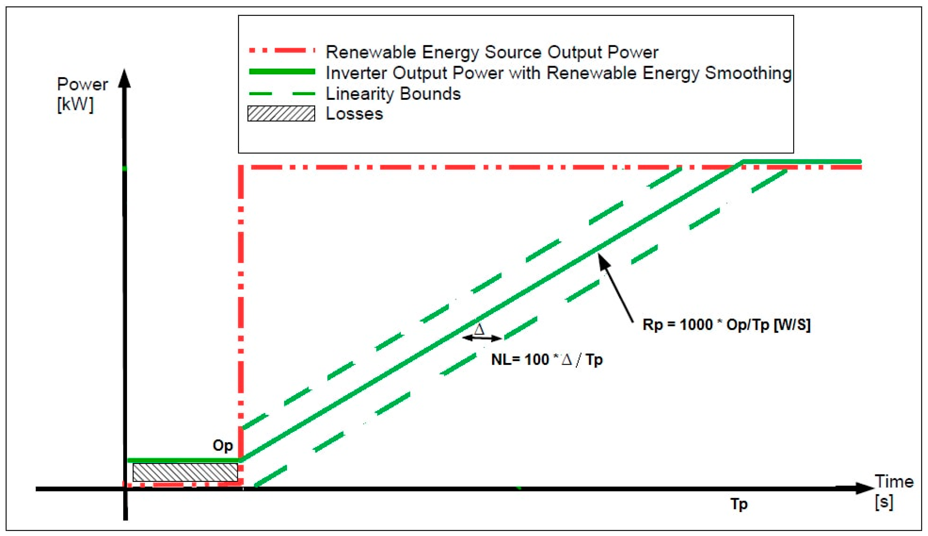
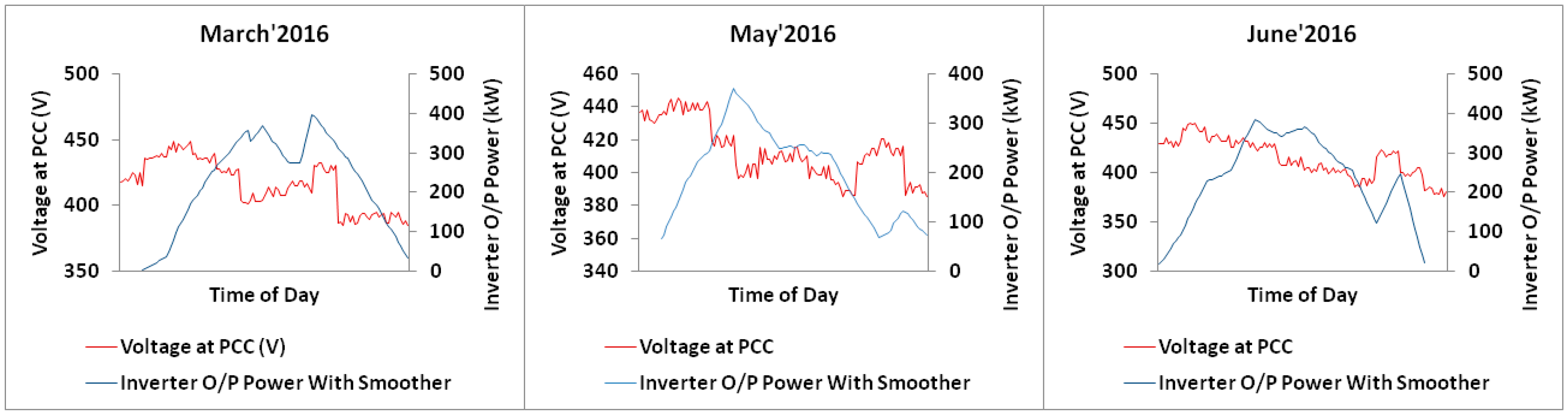
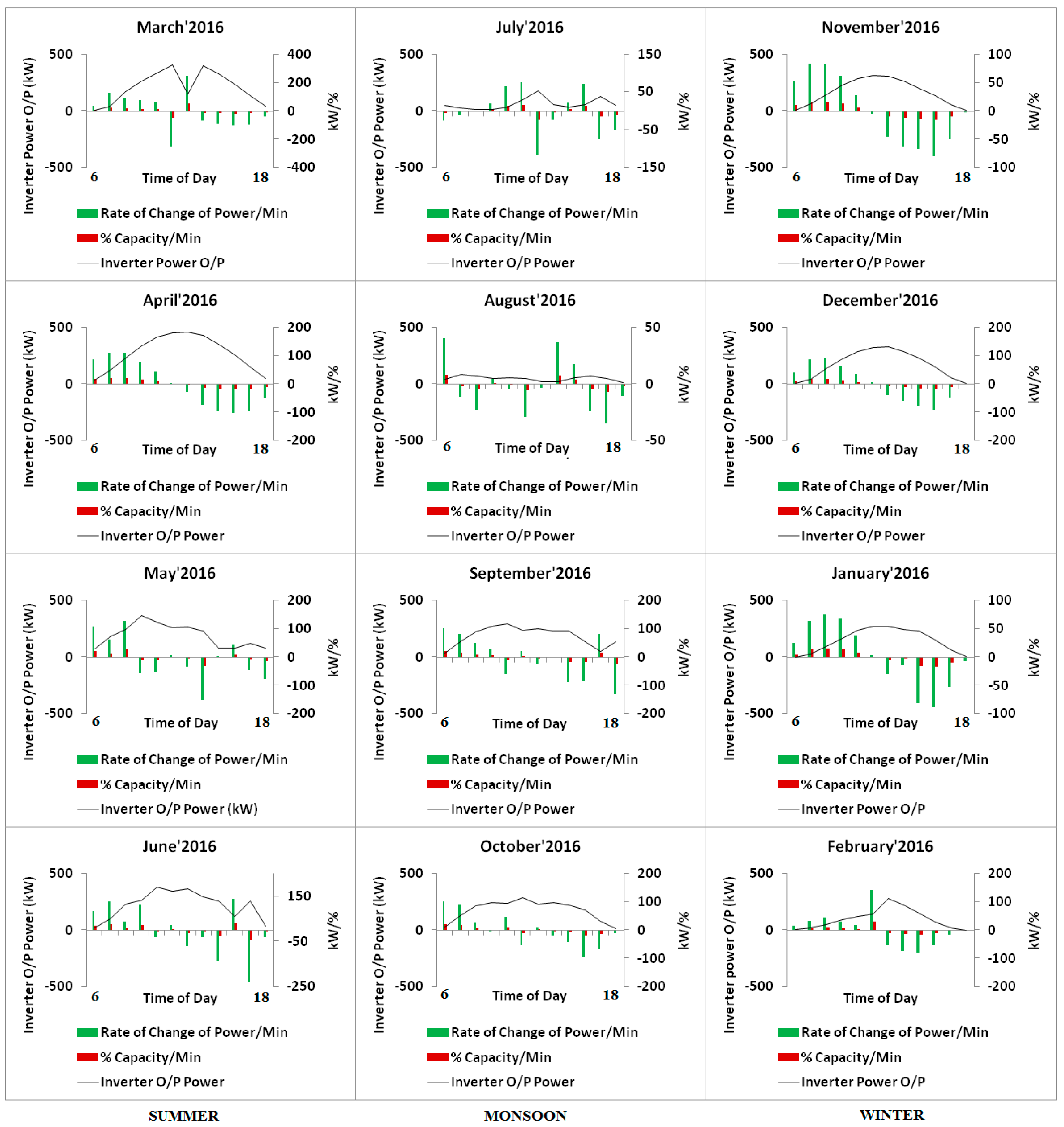
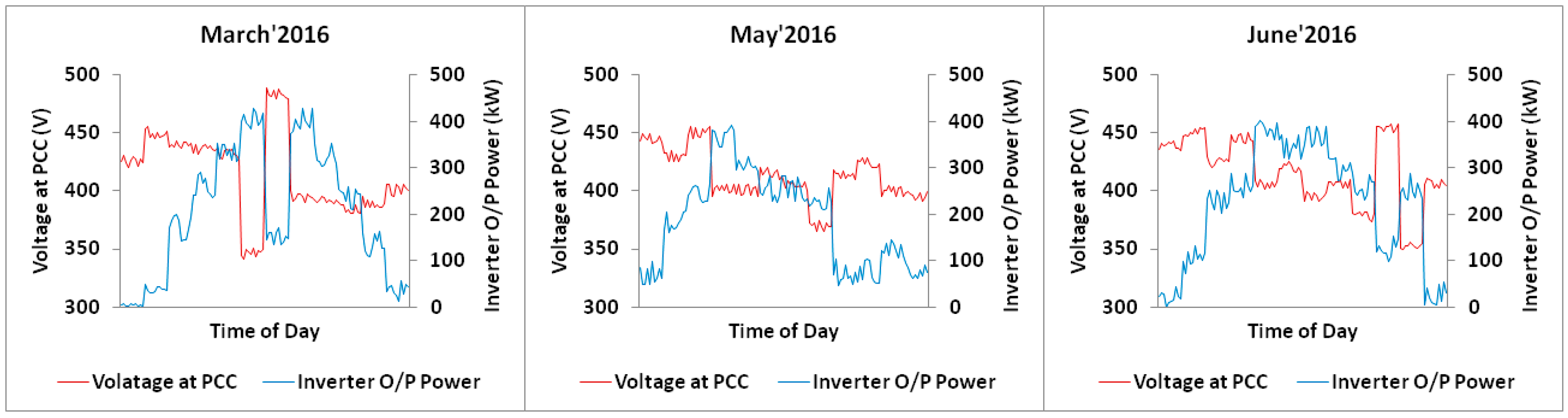
Further, the proposed solar smoother technology helps in minimizing significant electricity tariff financial losses by mitigating the probability of energy non-availability at the consumer end. The rest is divided into seven sections. This Section 1 describes the Introduction. Section 2 describes the effect of ramp up and ramp down of irradiance which leads to a voltage fluctuation in the distribution grid. 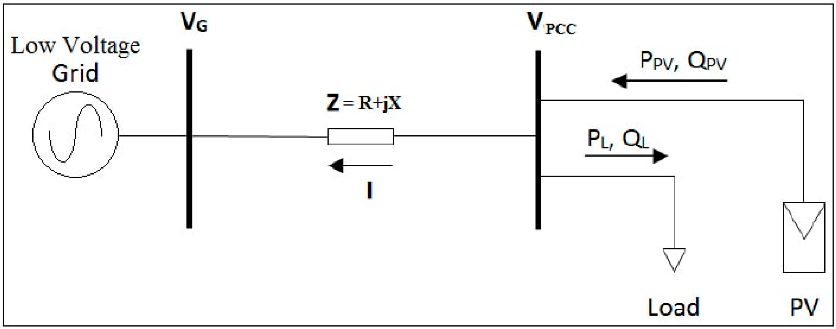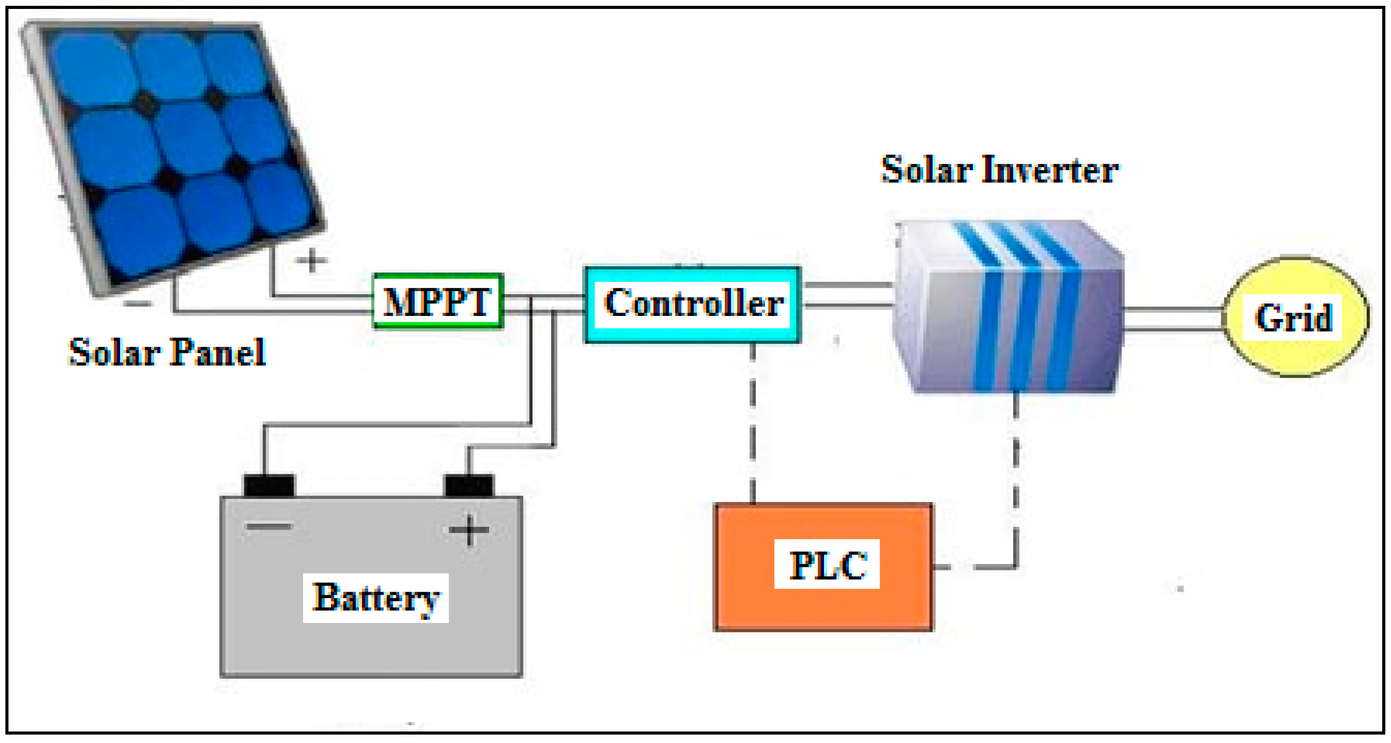Section 3 describes the modeling of the system. 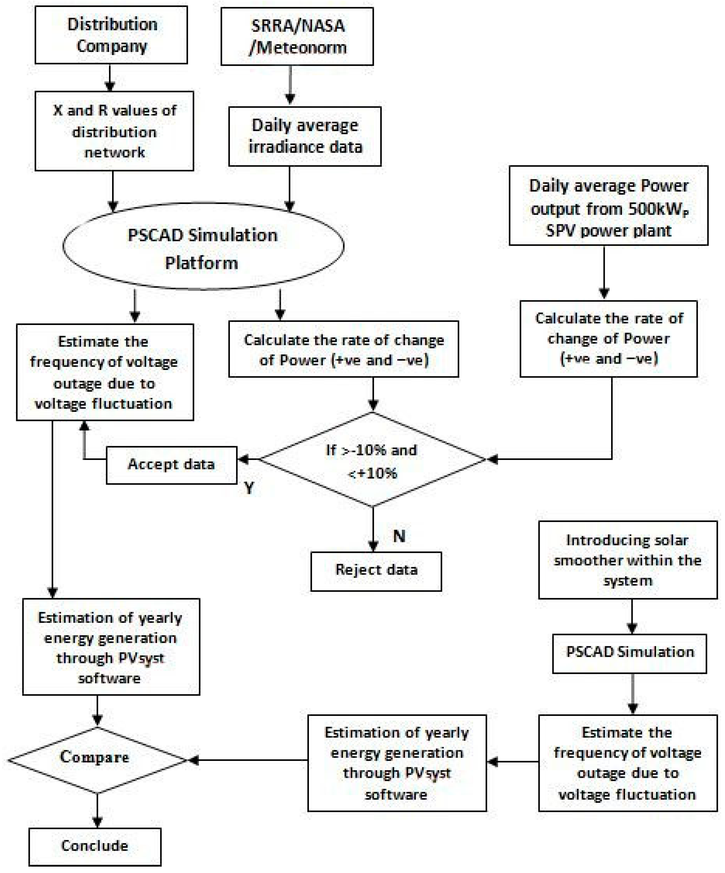Section 4 describes the methodology of the system. 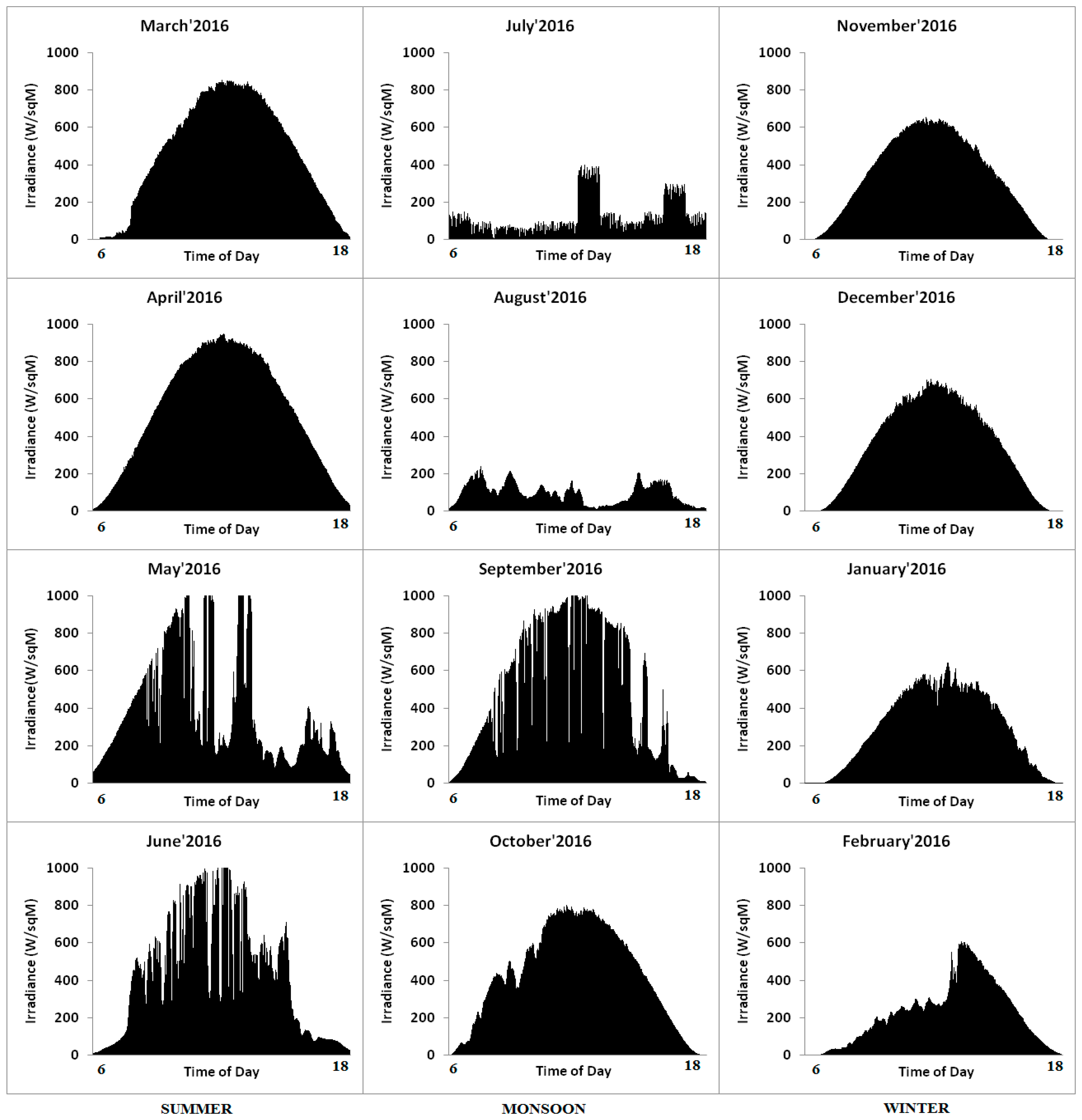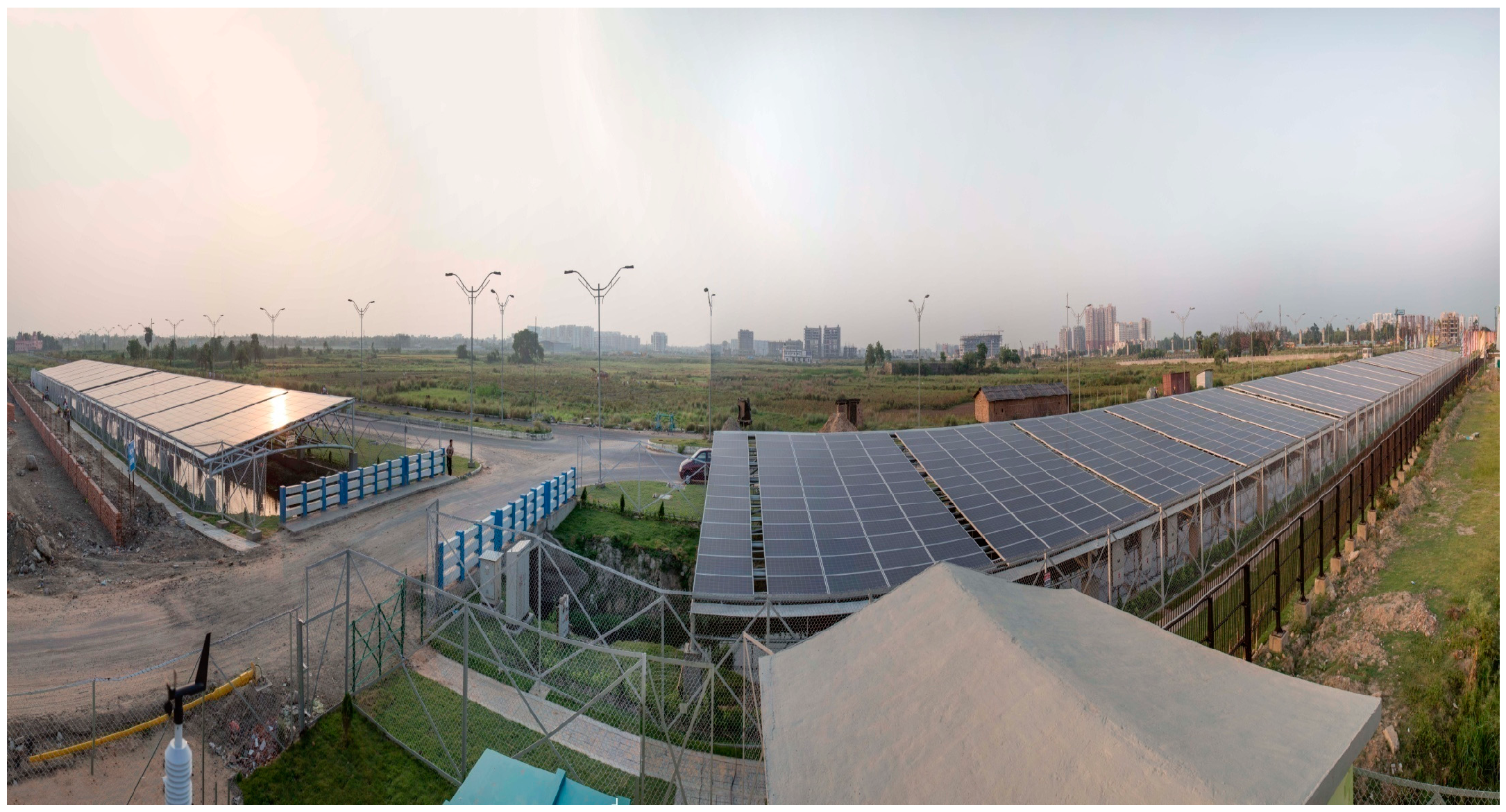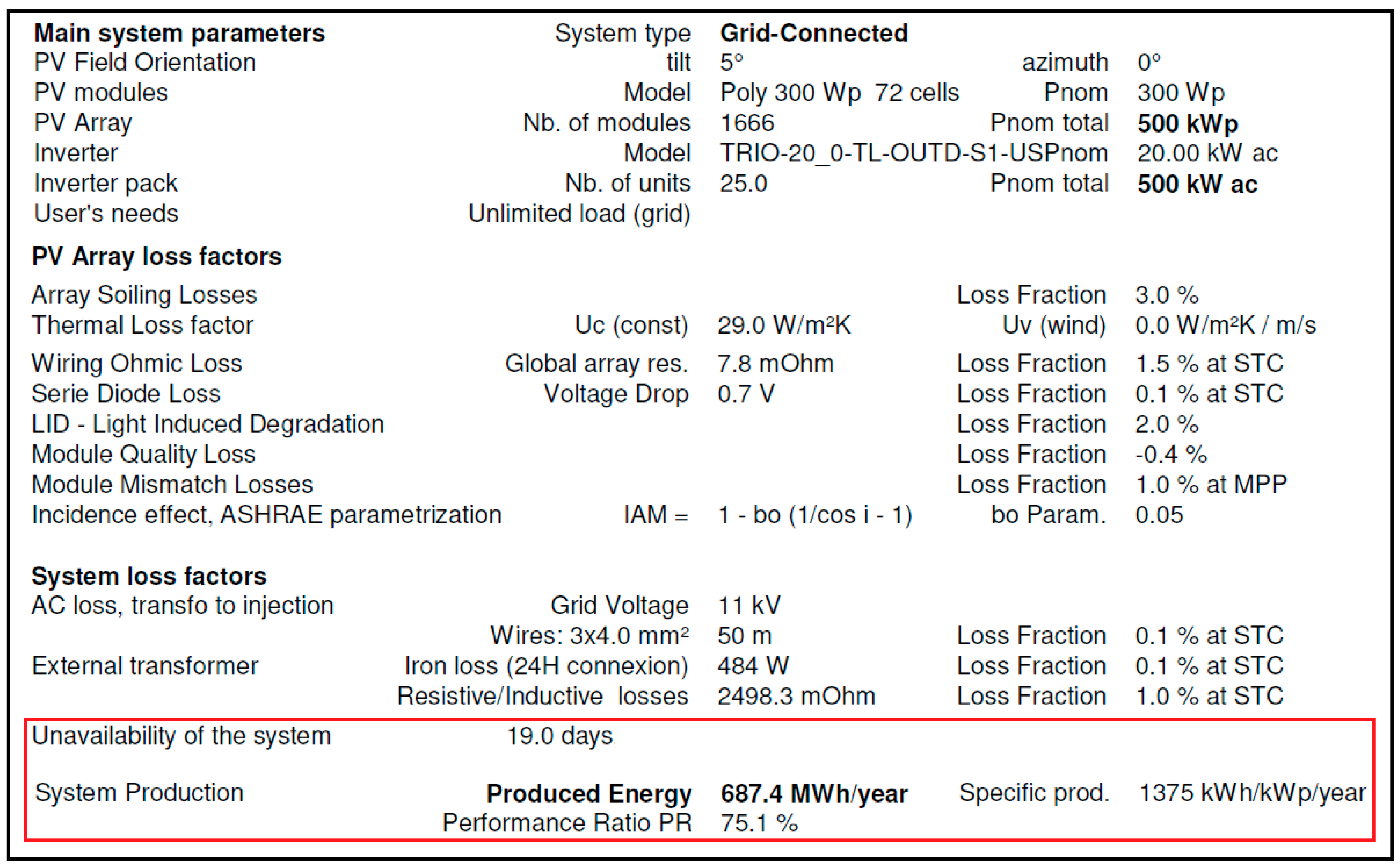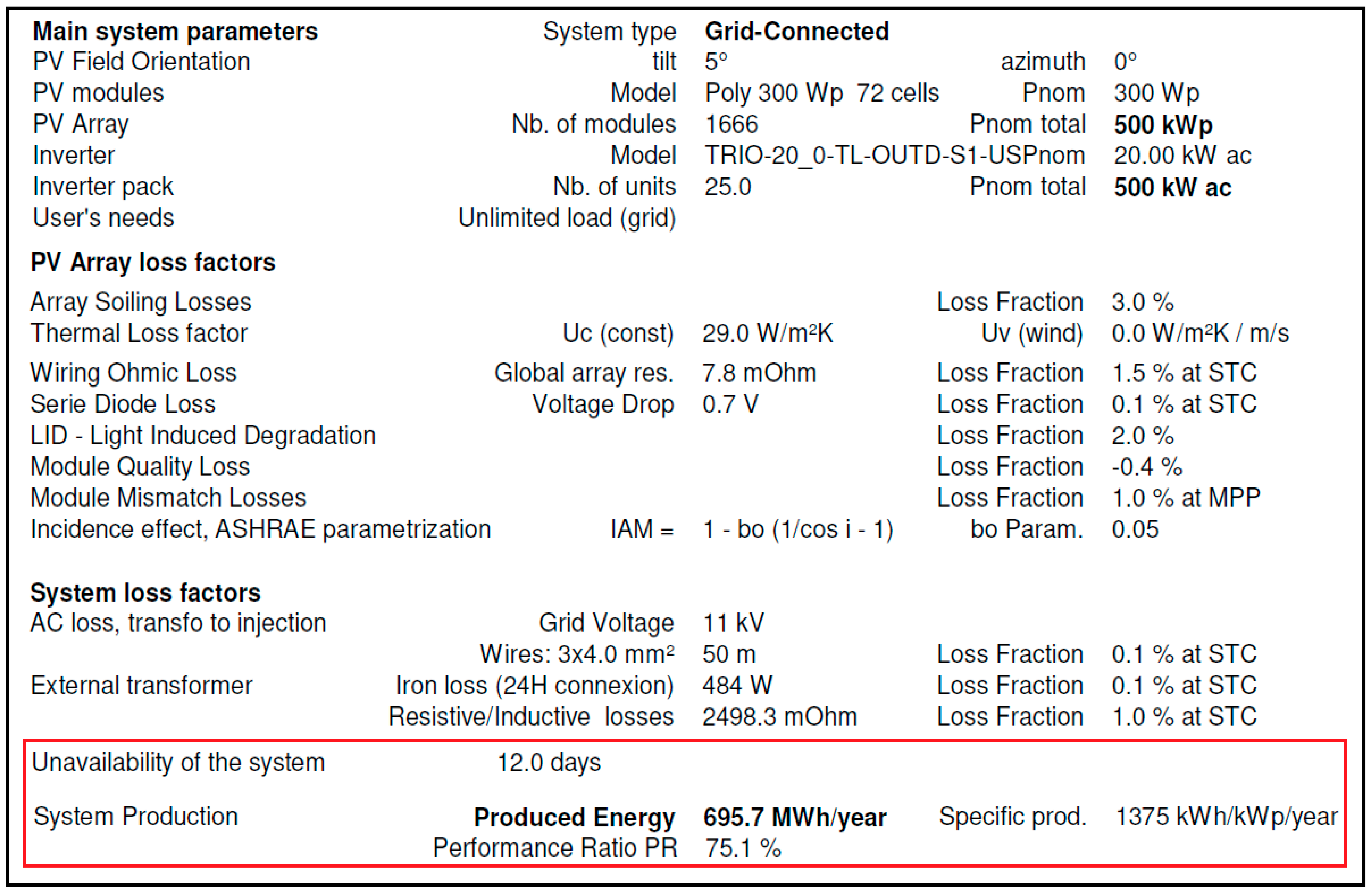Section 5 describes the case study of 500 kWp solar PV system installed in Kolkata, India, where the energy non-availability has been estimated using the proposed methodology and then validated though actual observations of field data. Section 6 discusses the financial issues. Section 7 presents the conclusions of the paper.

2. Effect of Irradiance Ramp up and Ramp down on a Solar Power Plant

2.1. Concept

Sudden variations of solar irradiance due to cloud passing are called ramp up and ramp down phenomena. When the ramp up and ramp down of irradiance occurs within a short amount of time, the inverter output power also fluctuates suddenly and voltage instability occurs at the point of common coupling of the distribution grid. To prevent the possibility of damage caused by instability, the usual practice is to curtail the connected load which leads to non-availability of energy. This method is not very efficient. A state of the art method called solar smoothing has been introduced to handle this situation. Due to increasing usage and penetration of solar PV in distribution grid the occurrence of such instability increases. On the other hand the solar energy providers have to guarantee the energy availability to the grid for long period of 20 years or more. Therefore it is most important for a solar energy provider to estimate correctly the frequency and duration of non-availability for a particular power plant over its lifetime and also use of smoothing for mitigation of this problem.

2.2. Characteristic Curve

Figure 1 shows the characteristic ramp down curve of the output power of a grid-connected inverter. The characteristic curve is defined as the desired output behavior of the grid-connected inverter, initially operating at nominal rated output, in response to a step change in renewable energy source output at time t = 0 s to 0 kW.

The ramp down phenomena can be established mathematically as:

$$R_n=-1000\times \left(\frac{Q_n}{T_n}\right)\mathrm{W}/\mathrm{s}$$

(1)

and,

$$NL=-1000\times \left(\frac{\Delta }{T_n}\right)\%$$

(2)

where R_n is the nominal ramp down rate (W/s), T_n is the nominal ramp down time (s), O_n is the nominal rated inverter output (kW), Δ is the maximum input deviation (s) and NL is the percentage of no linearity (%).

The nominal ramp down rate for each installation size is then derived according to Equation (2). Control action is required when the ramp down rate of the renewable energy source exceeds R_n in magnitude.

Similarly, the nominal ramp up time R_p is defined as the time taken for the inverter to ramp up from 0 kW to the nominal rated output, given by the following expression:

$$R_p=1000\times \left(\frac{Q_n}{T_p}\right)$$

(3)

Figure 2 describes the ramp up phenomena. This covers for sudden increase in renewable source electricity output. Control action is required when the ramp up rate of the renewable energy source exceeds R_p in magnitude.

3. Mathematical Model of the System

Figure 3 indicates the schematic diagram of a solar PV system connected with a low voltage distribution grid and load.

The PV and load are connected at point of common coupling (PCC) and the grid is connected through a distribution line to the PCC. The power generated from solar PV will be consumed by the load and the excess power, if any, will be exported to the grid. V_PCC indicates the voltage at the PCC at PV end, V_G indicates the grid voltage at point of supply from the distribution company, I is the PV current, Z is the impedance of the distribution line at the consumer end. The voltage deviation (∆V) can be expressed as:

$$\Delta V=V_{PCC}-V_G$$

(4)

Now, ΔV can be represented by Equation (5):

$$\Delta V\approx \frac{R\left[\left(P_{PV}-P_L\right)+\left(P_{PV}tan\alpha -P_{L}tan\varnothing \right)\left(\frac{X}{R}\right)\right]}{V_G}$$

(5)

where ϕ is the angle between the load voltage and load current, R_L is the load resistance (Ω) and α is the angle between V_PCC and I.

For ramp down phenomena Equation (6) can be written as:

$$V_{PCC}\approx V_G-\frac{R{V}_G}{R_L}\left[\left(\frac{R_n{T}_n}{1000P_L}+1\right)+\left(\frac{R_n{T}_n}{1000P_L}tan\alpha +tan\varnothing \right)\left(\frac{X}{R}\right)\right]$$

(6)

For ramp up phenomena Equation (7) can be written as:

$$V_{PCC}\approx V_G+\frac{R{V}_G}{R_L}\left[\left(\frac{R_n{T}_n}{1000P_L}-1\right)+\left(\frac{R_n{T}_n}{1000P_L}tan\alpha -tan\varnothing \right)\left(\frac{X}{R}\right)\right]$$

(7)

Therefore, Equations (6) and (7) describe that with a high ramp down rate of the inverter output power, the voltage at the PCC will dip, whereas with a high ramp up rate of the inverter output power the voltage at the PCC will rise.

4. Methodology

The methodology adopted for this work is as follows: first the month wise daily average irradiance data of the site is to be collected from a state of the art weather monitoring station located nearby. Otherwise National Aeronautics and Space Administration (NASA) or Meteonorm data may be used for this purpose, as shown in Figure 4. Various research papers [13,14,15] have also been published so far regarding the forecasting of solar power which can be also very useful for designing the prediction model.

The monthly average of the daily variation of power output of the power plant during the daytime is to be collected from the remote monitoring system of the power plant under consideration and the rate of change of power on the positive as well as the negative side is to be calculated. Figure 5 shows the raw data of the remote monitoring unit of the power plant under consideration for the month of March 2016.

The maximum and minimum ramp up and ramp down of the inverter output power and the percentage variation of the capacity can also be estimated from this raw data, as shown in Figure 5, but the voltage fluctuation at the PCC cannot be obtained directly.

Standard simulation software like PSCAD has been utilized in this work to estimate the voltage fluctuation. However for this purpose the simulation of the PSCAD needs to be validated with the field data of the power output variation. The X and R values of the distribution line are needed for carrying out the PSCAD simulation, which are to be collected from the distribution grid authority.

The voltage fluctuation at the PCC is estimated due to the heavy ramp up and ramp down of irradiance. The frequency and duration of voltage outages throughout the year can thus be estimated, from where the percentage loss of power supply is calculated. By using the PVsyst software the yearly generation has to be determined considering the calculated percentage of loss of power supply.

Similarly, by incorporating the solar smoother along with battery storage within the system, the voltage fluctuation at the PCC has to be identified and the frequency of voltage outage estimated through PSCAD simulation. The energy generation throughout the year has to be estimated by PVsyst simulation and compared with the previous one. Figure 6 shows the flow chart of the whole work.

5. Case Study

To validate the abovementioned methodology a case study has been performed. As shown in Figure 7, a 500 kWp grid tied solar PV plant located at Newtown Kolkata (India) was commissioned in 2015. It consists of a 500 kWp solar PV array, 25 × 20 kVA grid tied string inverters and 11 kV/0.415 kV, 650 kVA distribution transformers for connecting to the Newtown Electric Supply Company Ltd. (West Bengal, India) (NTESCL)’s local distribution network through a suitable protection system.

5.1. Month Wise Daily Average Irradiance Measurement

Figure 8 depicts the daily average Global Horizontal Irradiance (GHI) pattern of Kolkata in three different seasons, e.g., summer (March, April, May and June), monsoon (July, August, September and October) and winter (November, December, January and February) along with the rate of change of irradiance from 6:00 a.m. to 6:00 p.m. each day.

As the fluctuation of solar irradiance shows a maximum in summer and a minimum in winter, Figure 8 has been arranged accordingly e.g., it starts from March and ends in February. The irradiance data has been collected from the Solar Radiation Resource Assessment (SRRA) unit installed at the Indian Institute of Engineering Science and Technology (IIEST), Shibpur (India) campus. It is shown that the maximum rate of change of irradiance on the positive as well as negative side occurs mostly in the summer season and the maximum values are found in the months of March, May and June.

5.2. Month Wise Daily Average Inverter Output Power

In this work, a 1 min ramp rate is defined as the absolute value of the difference between the instantaneous power at the start and at the end of a 1 min period. The ramp rates over different time scales (Δt) can be calculated using the equation below:

$$\mathrm{Ramp}\mathrm{rate}=\frac{P\left(t_0\right)-P\left(t_0+\Delta t\right)}{\Delta t}$$

(8)

where P(t) is the time history of the inverter output power to the grid with measurements taken at t (in s) and Δt is the time interval. The daily average power output of each month from the plant measured at the point of common coupling (PCC) is shown in Figure 9.

It also shows the rate of change of power/min and the change of percentage capacity of the plant/min, on both the positive and negative side

Table 1. Month wise ramp up of inverter output power shown in surge zones.

SURGE ZONE (SZ)
	1 (NEAR 10%)		2 (NEAR 20%)		3 (NEAR 30%)		4 (NEAR 40%)		5 (NEAR 50%)		6 (NEAR 60%)
Month	Rate of Change of Power (kW)/min	% Change of Capacity/min	Rate of Change of Power (kW)/min	% Change of Capacity/min	Rate of Change of Power (kW)/min	% Change of Capacity/min	Rate of Change of Power (kW)/min	% Change of Capacity/min	Rate of Change of Power (kW)/min	% Change of Capacity/min	Rate of Change of Power (kW)/min	% Change of Capacity/min
January	37.50	7.50	75.00	15	-	-	-	-	-	-	-	-
February	42.50	8.50	-	-	139.5	27.9	-	-	-	-	-	-
March	35.5	7.1	94.5	18.9	128	25.6	-	-	248	49.6	-	-
April	42	8.4	85	17	108.5	21.7	-	-	-	-	-	-
May	42.5	8.5	60.5	12.1	125.5	25.1	-	-	-	-	-	-
June	35.5	7.1	84.5	16.9	137	27.4	-	-	-	-	-	-
July	22	4.4	75	15	-	-	-	-	-	-	-	-
August	40	8	-	-	-	-	-	-	-	-	-	-
September	50	10	80	16	101	20.2	-	-	-	-	-	-
October	47.5	9.5	90	18	102	20.4	-	-	-	-	-	-
November	27.5	5.5	83	16.6	-	-	-	-	-	-	-	-
December	41.5	8.3	91	18.2	-	-	-	-	-	-	-	-

and

Table 2. Month wise ramp down of inverter output power shown in surge zones.

SURGE ZONE (SZ)
	1 (NEAR 10%)		2 (NEAR 20%)		3 (NEAR 30%)		4 (NEAR 40%)		5 (NEAR 50%)		6 (NEAR 60%)
Month	Rate Of Change of Power (kW)/min	% Change of Capacity/min	Rate of Change of Power (kW)/min	% Change of Capacity/min	Rate of Change of Power (kW)/min	% Change of Capacity/min	Rate of Change of Power (kW)/min	% Change of Capacity/min	Rate of Change of Power (kW)/min	% Change of Capacity/min	Rate of Change of Power (kW)/min	% Change of Capacity/min
January	−29.50	−5.90	−88.00	−17.6	-	-	-	-	-	-	-	-
February	−15.90	−3.18	−81	−16.2	-	-	-	-	-	-	-	-
March	−40.5	−8.1	−95	−19	−101.5	−20.3	-	-	-	-	−253.5	−50.7
April	−29	−5.8	−97.5	−19.5	−104	−20.8	-	-	-	-	-	-
May	−45	−9	−76.5	−15.3	-	-	−152.5	−30.5	-	-		-
June	−33.5	−6.7	−71	−14.2	−137	−27.4	-	-	−228	−45.6	-	-
July	−26	−5.2	−74	−14.8	−118.5	−23.7	-	-	-	-	-	-
August	−29	−5.8	-	-	-	-	-	-	-	-	-	-
September	−25	−5	−87.5	−17.5	−130.5	−26.1	-	-	-	-	-	-
October	−43.5	−8.7	−97.5	−19.5	-	-	-	-	-	-	-	-
November	−50	−10	−79.5	−15.9	-	-	-	-	-	-	-	-
December	−49	−9.8	−93.5	−18.7	-	-	-	-	-	-	-	-

show the month wise ramp up and ramp down of inverter output power which has been divided in six surge zones (SZ) e.g., from SZ-1 (10% change of capacity/min) to SZ-6 (60% change of capacity/min).

It is noticed from Table 1 and Table 2 that the low ramp up and ramp down of inverter power (up to 30%) occurs mostly in every month whereas the high ramp up (up to 50%) occurs in the month of March and the high ramp down (up to 40%, 50% and 60%) occurs in the months of May, June and March, respectively.

5.3. PSCAD Simulation

The above said 500 kWp solar PV system connected to the low voltage NTSCL distribution grid has been simulated through the PSCAD software. The simulation describes the level of power surge of the inverter output within the distribution network with values of the X/R ratio of the distribution line. A boundary limit of the grid voltage has also been identified beyond which the grid becomes unstable. A test network model for low voltage distribution line has been developed in PSCAD. The X and R values (0.205 + j0.074) of the network are collected from NTSCL and fed to the simulation along with the irradiance data. The simulation has been done with six different power surge zones to observe the voltage fluctuation level at PCC.

Table 3. Comparison between real time and simulated data.

	Month
	March			May			June
Time of Day	Simulated	Realtime	% Deviation	Simulated	Realtime	% Deviation	Simulated	Realtime	% Deviation
6:00	7.1	6.9	3.6	21.1	21.7	−2.8	16.9	16.3	3.6
7:00	25.6	25.5	0.5	12.1	12.0	0.5	25.4	25.3	0.5
8:00	18.9	18.6	1.5	25.1	24.7	1.5	7.1	7.8	−9.0
9:00	15.0	15.8	−5.1	−11.2	−10.4	7.7	22.3	23.0	−3.0
10:00	13.2	12.5	5.8	−10.9	−10.3	5.8	−6.7	−6.3	5.8
11:00	−50.7	−48.4	4.7	1.4	1.5	−6.7	4.3	4.1	4.7
12:00	49.6	50.3	−1.4	−6.6	−6.9	−4.3	−14.2	−13.3	7.0
13:00	−13.9	−14.2	−2.1	−30.5	−30.0	1.5	−6.7	−7.1	−5.6
14:00	−18.3	−17.5	4.7	0.8	0.8	4.7	−27.4	−26.2	4.7
15:00	−20.3	−19.6	3.6	8.5	8.2	3.6	27.4	26.4	3.6
16:00	−19.0	−20.9	−9.1	−9.0	−9.8	−8.2	−45.6	−44.5	2.6
17:00	−8.1	−7.7	4.7	−15.3	−14.6	4.7	−6.1	−6.7	−9.0

shows the comparison between the percentage change of capacity/min between real time data obtained from 500 kWp solar PV plant and PSCAD simulation along with the percentage deviation for three months, namely March, May and June. It shows that the maximum deviation on the positive side is 7.7% and on the negative side it is −9.1%, which are well between ±10%. This validates the simulation results.

Figure 10 shows the inverter output power and voltage at PCC for the months of March, May and June which cover the six surge zones described above. It clearly shows the voltage swelling and sagging at the PCC at the time of ramp up and ramp down of the inverter output power.

Table 4. Voltage at PCC against % change of inverter output/min.

March		May		June
% Change of Capacity/min	Voltage at PCC (V)	% Change of Capacity/min	Voltage at PCC (V)	% Change of Capacity/min	Voltage at PCC (V)
7.1	425	21.1	444	16.9	438
25.6	450	12.1	432	25.4	450
18.9	441	25.1	450	7.1	425
15.0	436	−11.2	400	22.3	446
13.2	433	−10.9	400	−6.7	406
−50.7	345	1.4	417	4.3	421
49.6	484	−6.6	406	−14.2	395
−13.9	396	−30.5	373	−6.7	406
−18.3	390	0.8	416	−27.4	377
−20.3	387	8.5	427	27.4	453
−19.0	389	−9.0	403	−45.6	352
−8.1	404	−15.3	394	−6.1	407

shows the simulated values of voltage at the PCC against the percentage change of inverter output (in power/min). The portions marked in red in the table show the swelling and sagging values of the PCC voltages which are beyond the tolerable limit on both the positive and negative side. The tolerable voltage limit has been considered as per Indian Grid Code i.e., ±10% of rated voltage (400 V AC). From Table 3 the ramp up and ramp down allowable limits of the inverter output power have been calculated as 17%/min and 46%/min, respectively.

5.4. Estimation of Energy Non Availability through PVsyst Simulation without Smoothing

In

Table 5. Frequency of occurrence of ramp up and ramp down of inverter output power/min.

January	February	March	April	May	June	July	August	September	October	November	December
4.92	3.1	7.1	17	21.1	16.9	−5.2	8	20.2	20.4	10.5	8.3
12.6	6.2	25.6	21.7	12.1	25.4	−2	−2.3	16	18	16.6	17.5
15	8.5	18.9	21.6	25.1	7.1	0	−4.6	10	5.2	16.4	18.2
13.60	5.7	15	15.3	−11.2	22.3	4	0.9	5	−0.9	12.4	12.9
7.50	3.7	13.2	8.4	−10.9	−6.7	13	−1	−12	9.5	5.5	6.8
0.60	27.9	−50.7	0.4	1.4	4.3	15	−5.8	3.9	−10.7	−1.1	1.4
−5.90	−10.8	49.6	−5.8	−6.6	−14.2	−23.7	−0.7	−5	2	−9.2	−8.1
−2.80	−14.6	−13.9	−15.1	−30.5	−6.7	−4.8	7.4	−0.6	−4	−12.5	−12
−16.20	−16.2	−18.3	−19.5	0.8	−27.4	4.4	3.5	−17.5	−8.7	−13.5	−16.2
−17.60	−10.6	−20.3	−20.8	8.5	27.4	14.1	−4.9	−17.1	−19.5	−15.9	−18.7
−10.50	−3.18	−19	−19.4	−9	−45.6	−14.8	−7	16	−13.8	−10	−9.8
−1.30	−0.02	−8.1	−10.2	−15.3	−6.1	−10.2	−2.2	−26.1	−2	−0.5	−0.6

the portions marked in blue show the frequency of occurrence of ramp up and ramp down of the inverter output power/min beyond the tolerable limit on the positive as well as the negative side, which is calculated as 13.19% throughout the year. Conversely, it can be considered that the year-round energy availability of the system is 86.81%.

A PVsyst-based simulation has been done to estimate the power generation throughout the year considering the loss of load 13.19%. This is illustrated in Figure 11.

It is shown from the figure that the total energy generation is 687.4 MWh against a Performance Ratio (PR) value of 75.1%. The energy unavailability from the system is 19 days in a year.

5.5. Proposed Implication on Energy Estimation with Smoother Incorporating Energy Storage

A proposal has been presented where by incorporation of battery storage within the system, the availability of the power can be increased. At the time of ramp up the storage device will be in discharging mode and vice versa. The schematic of the system is indicated in Figure 12.

The system has been simulated in PSCAD maintaining the other parameters the same. The capacity of the storage can be designed to mitigate the maximum ramp up and ramp down rate throughout the year. Table 1 and Table 2 show that the maximum ramp rate of power is 248 kW/min on the positive side and 253.5 kW/min on the negative side. The maximum energy content within the surge will be:

$$E_{surge}=P_{surge}*t$$

(9)

where, P_surge = surge power in kW, and t = time up to when the surge exists in minutes.

From Equation (9) E_surge has been calculated as 4225 units. Now, this amount of energy will be absorbed by the battery storage at the time of ramp up and will be released at the time of ramp down phenomena. Moreover, from Table 5 it is noticed that a maximum three times a day in the month of April the power is fluctuating beyond the limit. Therefore to handle this surge power the energy at battery needs to be stored as:

$$E_{Battery}=E_{surge}*3$$

(10)

The capacity of the battery has been calculated as:

$$C_{Battery}=\frac{V_{Battery}}{E_{Battery}}$$

(11)

where, V_battery = terminal voltage of the battery bank.

In this case 684V DC is taken as the string voltage of the PV is nearly 700 V DC. Therefore from Equation (11) the capacity of the battery has been calculated as 18.53 Ah. Now, considering up to 85% depth of discharge (DOD) of the battery and availability in the market, the capacity has been taken as 22 Ah. In this case a Gel Long Life battery has been considered. Fifty seven 12 V, 22 Ah battery modules have been connected in series to provide a terminal voltage of 684 V DC [20].

After incorporation of the smoother and storage the output of the inverter power and voltage at the PCC is as shown in Figure 13.

In comparison to Figure 10, it is shown in Figure 13 that after incorporation of the storage system along with the smoother, the ramp up and ramp down rate of the inverter output power has been smoothed out and the corresponding voltage fluctuation has also been minimized.

Table 6. Voltage at PCC against % change of inverter output/min after introduction of a solar smoother.

March		May		June
% Change of Capacity/min	Voltage at PCC (V)	% Change of Capacity/min	Voltage at PCC (V)	% Change of Capacity/min	Voltage at PCC (V)
4.0	421	10.83	431	8.96	427
19.7	440	17.73	437	22.1	446
19.3	443	17.48	443	15.62	437
14.7	438	4.33	423	16.52	438
11.6	429	−10.28	399	6.18	424
−6.3	404	−4.1	406	−0.99	414
−1.6	415	−0.97	412	−5.37	408
8.5	426	−11.15	400	−10.5	400
−15.1	394	−16.2	392	−18.3	390
−18.2	388	−0.97	413	2.71	419
−20.9	388	−0.4	413	−14.06	396
−16.5	392	−21.06	390	−25.67	379

shows the values of voltage at the PCC against the percentage change of inverter output power/min.

After introduction of the smoother the voltage swelling and sag at the PCC is reduced significantly. The minimum and maximum voltage fluctuation are increased from 345 V and 484 V revives up to 404 V and 415 V, respectively.

Table 7. Occurrence of ramp up and ramp down of inverter output power/min after introduction of a solar smoother.

January	February	March	April	May	June	July	August	September	October	November	December
3.3	1.5	3.6	8.8	11.4	9.3	−2.3	3.0	11.0	10.6	6.6	6.4
8.8	5.1	17.3	20.4	16.3	20.2	−3.4	1.3	18.5	18.4	14.5	13.7
14.8	7.0	21.9	21.0	19.1	16.7	−2.4	−2.1	13.5	11.6	16.0	17.9
14.2	6.5	15.5	17.6	4.4	13.7	3.6	−1.3	6.5	1.6	12.9	15.7
10.5	4.9	10.9	11.3	−10.7	6.3	8.5	−1.0	−5.4	5.3	8.1	8.5
4.8	17.6	−7.5	4.2	−6.0	1.1	14.2	−4.0	−1.8	−2.9	1.4	3.3
−3.0	6.6	−1.0	−2.3	−1.6	−6.4	−6.2	−3.5	−1.1	−4.8	−4.6	−3.5
−6.0	−13.7	11.5	−9.8	−10.2	−9.2	−13.0	4.0	−2.9	−0.5	−9.5	−10.5
−11.9	−14.0	−17.8	−19.2	−15.5	−17.8	1.2	6.3	−9.6	−6.3	−13.0	−12.9
−15.7	−12.9	−18.6	−20.9	−1.2	2.2	8.5	−1.7	−16.8	−14.3	−14.7	−17.7
−11.6	−8.1	−19.9	−18.7	−2.2	−13.9	−3.9	−4.3	2.2	−17.9	−13.6	−15.2
−7.6	−1.0	−16.8	−19.1	−18.9	−26.0	−14.4	−7.8	−20.9	−6.9	−5.2	−4.8

shows the frequency of occurrence of ramp up and ramp down of the inverter output power/min beyond the tolerable limit on positive as well as the negative side.

In Table 7 the portions marked in blue show the frequency of occurrence of ramp up and ramp down of the inverter output power/min beyond the tolerable limit in the positive as well as the negative direction after introduction of the smoother, calculated as 8.33% throughout the year. Thus from the point of view way it can be considered that the year-round availability of the system is 90%. In comparison to Table 4 it shows that the availability of the system is improved up to 4.86% throughout the year. Similarly a PVsyst report has been generated considering 10% availability factor and the result is presented in Figure 14.

From Figure 11 and Figure 14 it is seen that the energy production has been increased from 687.4 MWh/year to 695.7 MWh/year.

6. Financial Issues

The financial aspect is one of the major concerns of a solar power plant which eventually depends on the loss of energy due to system unavailability. The developer of a solar power plant earns revenue by selling energy to the distribution company against a declared tariff decided by the Central Electricity Regulatory Commission in India.

Thus it would be desirable to generate more energy to earn more revenue which in turn increases the project viability. The unavailability of the system increases the loss of energy, followed by a loss of earned revenue.

Table 8. Cost and bill of material for 500 kWp solar PV plant without solar smoother and battery.

Sl. No.	Item	Specification	Total Cost (INR)
1	Solar PV Module	500 kWp (300 Wp × 1667 nos.)	2.25 Crore
2	Solar Inverter with remote monitoring system	500 kW (20 kW × 25 nos.)
3	Structure & Accessories	33 ton Iron Structure
4	Junction Boxes	100 kW × 5 nos.
5	LT Panel with Energy Meter	500 KW
6	Cable and Accessories	Suitable Cross Section
7	Plant Protection System	Earthing, Surge and Lightning
8	Installation and Commissioning	500 kW
9	Operation & Maintenance	for 10 years	0.50 Crore
TOTAL			2.75 Crore

above describes the investment for a 500 kWp solar PV plant without a solar smoother.

The total investment including installation and commissioning, operation & maintenance for 10 years is around Indian Rupee (INR) 27.5 million (INR 2.75 CR), as shown in Table 8. The assumptions are as follows:

• Solar module efficiency degradation = 1% per year
• Net metering tariff adjusted = INR 10.25/kWh [21]
• Escalation of power tariff = 5% per year
• Accelerated Depreciation Benefit = 80% in first year
• Tax implication = 30%

Table 9. Cash flow for a 10 year period without a solar smoother and battery.

Year	1	2	3	4	5	6	7	8	9	10
Energy Generation (kWh)	687,400	680,526	673,652	666,778	659,904	653,030	646,156	639,282	632,408	625,534
Tariff (INR)	10.25	10.76	11.30	11.87	12.46	13.08	13.74	14.42	15.14	15.90
Realization (INR)	7,045,850	7,324,161	7,612,689	7,911,759	8,221,704	8,542,864	8,875,586	9,220,223	9,577,135	9,946,688
Accelerated Depreciation (INR)	5,220,000	145,000	145,000	145,000	145,000	145,000	145,000	145,000	145,000	145,000
Realization After Depreciation (INR)	12,265,850	7,469,161	7,757,689	8,056,759	8,366,704	8,687,864	9,020,586	9,365,223	9,722,135	10,091,688
Tax Deduction (INR)	2,113,755	2,197,248	2,283,807	2,373,528	2,466,511	2,562,859	2,662,676	2,766,067	2,873,141	2,984,006
Realization After Tax (INR)	10,152,095	5,271,913	5,473,882	5,683,231	5,900,193	6,125,005	6,357,910	6,599,156	6,848,995	7,107,681
Net Cumulative Realization (INR)	10,152,095	15,424,008	20,897,890	26,581,121	32,481,313	38,606,318	44,964,228	51,563,385	58,412,379	65,520,061

shows the cumulative revenue from selling power for ten years is INR 65,520,061/-, considering accelerated depreciation benefit and income tax deduction against an investment of INR 27,500,000/-.

Now, by retrofitting the solar smoother and the battery bank in the system the material cost has been increased by INR 11.5 Lac, where the cost of the battery bank is INR 10.0 Lac and the cost of the smoother circuits with protections is INR 1.5 Lac. Therefore the cost of the whole system including solar smoother, battery bank and its replacement two times in ten years has become INR 30,650,000/-.

Table 10. Cost and bill of material for a 500 kWp solar PV plant with solar smoother and battery.

Sl. No.	Item	Specification	Total Cost (INR)
1	Solar PV Module	500 kWp (300 Wp × 1667 nos.)	2.365 Crore
2	Solar Inverter with remote monitoring system	500 kW (20 kW × 25 nos.)
3	Structure & Accessories	33 ton Iron Structure
4	Junction Boxes	100 kW × 5 nos.
5	LT Panel with Energy Meter	500 KW
6	Cable and Accessories	Suitable Cross Section
7	Solar Smoother with Accessories	Controller & PLC
8	Battery Bank	12 V, 20 Ah × 57 nos.
9	Plant Protection System	Earthing, Surge and Lightning
10	Installation and Commissioning	500 kW
11	Operation & Maintenance	for 10 years	0.50 Crore
12	Battery Replacement cost	Every 5 years, i.e., 2 times within 10 years	0.20 Crore
TOTAL			3.065 Crore

shows a detailed bill of materials and the specifications of each item.

Table 11. Cash flow for a 10 year period with solar smoother and battery.

Year	1	2	3	4	5	6	7	8	9	10
Energy Generation (kWh)	695,700	688,743	681,786	674,829	667,872	660,915	667,872	674,829	681,786	688,743
Tariff (INR)	10.25	10.76	11.30	11.87	12.46	13.08	13.74	14.42	15.14	15.90
Realization (INR)	7,130,925	7,412,597	7,704,608	8,007,289	8,320,977	8,646,015	9,173,877	9,732,910	10,324,911	10,951,781
Accelerated Depreciation (INR)	5,220,000	145,000	145,000	145,000	145,000	145,000	145,000	145,000	145,000	145,000
Realization After Depreciation (INR)	12,350,925	7,557,597	7,849,608	8,152,289	8,465,977	8,791,015	9,318,877	9,877,910	10,469,911	11,096,781
Tax Deduction (INR)	2,139,278	2,223,779	2,311,382	2,402,187	2,496,293	2,593,804	2,752,163	2,919,873	3,097,473	3,285,534
Realization After Tax (INR)	10,211,648	5,333,818	5,538,226	5,750,102	5,969,684	6,197,210	6,566,714	6,958,037	7,372,438	7,811,247
Net Cumulative Realization (INR)	10,211,648	15,545,465	21,083,691	26,833,793	32,803,476	39,000,687	45,567,400	52,525,437	59,897,875	67,709,122

, which shows the cash flow after incorporation of the solar smoother and battery bank in the system, indicates that the cumulative revenue has become INR 67,709,122/- from selling power for “ten” years against an investment of INR 30,650,000/-.

Therefore, the cumulative revenue increases significantly by INR 2,189,061/- after inclusion of the solar smoother and battery bank within the system which is about 20% of the net cumulative realization (INR) in the first year of the 500 kWp system. For larger systems of MW scale the benefit will be substantial.

7. Conclusions

In this paper, a generalized methodology has been proposed for estimation of the distribution grid dynamics under the impact of variable solar PV generation throughout the year using the PSCAD simulation platform. Further, the non-availability of energy at the grid end is estimated by fitting the PSCAD observations into a PVsyst model as input and this problem is mitigated by incorporating a solar smoother in the existing system. The model performance is validated by a practical 500 kWp solar PV power system. It has been found that the energy non-availability is reduced by 4.86% after inclusion of the solar smoother technology. Further, the economic impact of the proposed system has also been discussed. It has been found that by inclusion of a solar smoother in the existing power plant a significant excess revenue of around INR 218,000/- per month occurs by preventing the non-availability of energy during the inverter shutdowns caused by voltage fluctuations beyond the limit.

References

1. Kamaruzzaman, Z.A.; Mohamed, A.; Shareef, H. Effect of grid-connected photovoltaic systems on static and dynamic voltage stability with analysis techniques—A review. In Przegląd Elektrotechniczny; University Kebangsaan Malaysia: Selangor, Malaysia, 2015; pp. 134–138. [Google Scholar]
2. Alam, M.J.; Muttaqi, K.M.; Sutanto, D. A novel approach for ramp-rate control of solar PV using energy storage to mitigate output fluctuations caused by cloud passing. IEEE Trans. Energy Convers. 2014, 29, 507–518. [Google Scholar]
3. Jewell, W.; Ramakumar, R. The effects of moving clouds on electric utilities with dispersed photovoltaic generation. IEEE Trans. Energy Convers. 1987, 2, 570–576. [Google Scholar] [CrossRef]
4. Hoke, A.; Hambrick, R.B.J.; Kroposki, B. Maximum Photovoltaic Penetration Levels on Typical Distribution Feeders; National Renewable Energy Laboratory: Golden, CO, USA, 2012.
5. Wang, L.; Lin, Y.H. Dynamic stability analysis of a photovoltaic array connected to a large utility grid. In Proceedings of the IEEE PES Winter Meeting, Singapore, 23–27 January 2000; Volume 1, pp. 476–480. [Google Scholar]
6. Srisaen, N.; Sangswang, A. Effect of PV grid-connected system location on a distribution system. In Proceedings of the IEEE Asia Pacific Conference on Circuit and Systems, Singapore, 4–7 December 2006; pp. 852–855. [Google Scholar]
7. Johnson, R.; Johnson, L.; Nelson, L.; Lenox, C.; Stein, J. Methods of integrating a high penetration photovoltaic power plant into a micro grid. In Proceedings of the 35th IEEE Photovoltaic Specialists Conference, Honolulu, HI, USA, 20–25 June 2010; pp. 289–294. [Google Scholar]
8. Jayasekara, N.; Wolfs, P.; Masoum, M.A. An optimal management strategy for distributed storages in distribution networks with high penetrations of PV. Electr. Power Syst. Res. 2014, 116, 147–157. [Google Scholar] [CrossRef]
9. Yan, R.; Saha, T.K. Investigation of voltage stability for residential customers due to high photovoltaic penetrations. IEEE Trans. Power Syst. 2012, 27, 651–662. [Google Scholar] [CrossRef]
10. Marcos, J.; de la Parra, I.; García, M.; Marroyo, L. Control strategies to smooth short-term power fluctuations in large photovoltaic plants using battery storage systems. Energies 2014, 7, 6593–6619. [Google Scholar] [CrossRef]
11. Yan, R.; Saha, T.K. Power ramp rate control for grid connected photovoltaic system. In Proceedings of the 9th International Power and Energy Conference, Singapore, 27–29 October 2010. [Google Scholar]
12. Omran, W.A.; Kazerani, M.; Salama, M. Investigation of methods for reduction of power fluctuations generated from large grid-connected photovoltaic systems. IEEE Trans. Energy Convers. 2011, 26, 318–327. [Google Scholar] [CrossRef]
13. Barelli, L.; Bidini, G.; Bonucci, F.; Castellini, S.; Ottaviano, A.; Pelosi, D.; Zuccari, A. Dynamic analysis of a hybrid energy storage system (H-ESS) coupled to a photovoltaic (PV) plant. Energies 2018, 11, 396. [Google Scholar] [CrossRef]
14. Giraud, F.; Salameh, Z.M. Analysis of the effects of a passing cloud on a gridinteractive photovoltaic system with battery storage using neural networks. IEEE Trans. Energy Convers. 1999, 14, 1572–1577. [Google Scholar] [CrossRef]
15. Chalmers, S.M.; Hitt, M.M.; Underhill, J.T. The effect of photovoltaic power generator on utility operation. IEEE Trans. Power Appar. Syst. 1985, 104, 524–530. [Google Scholar] [CrossRef]
16. Datta, M.; Senjyu, T.; Yona, A.; Funabashi, T.; Kim, C.-H. Photovoltaic output power fluctuations smoothing methods for single and multiple PV generators. Curr. Appl. Phys. 2010, 10, S265–S270. [Google Scholar] [CrossRef]
17. Addisu, A.; George, L.; Courbin, P.; Sciandra, V. Smoothing of renewable energy generation using Gaussian-based method with power constraints. In Proceedings of the 9th International Conference on Sustainability in Energy and Building (SEB-17), Chania, Greece, 5–7 July 2017. [Google Scholar]
18. De la Parra, I.; Marcos, J.; García, M.; Marroyo, L. Control strategies to use the minimum energy storage requirement for PVpower ramp-rate control. Sol. Energy 2015, 111, 332–343. [Google Scholar] [CrossRef]
19. Sarkar, T.; Dan, A.K.; Ghosh, S.; Das Bhattacharya, K.; Saha, H. Interfacing Solar PV Power Plant with Rural Distribution Grid: Challenges and Possible Solutions. Int. J. Sustain. Energy 2017, 1–20. [Google Scholar] [CrossRef]
20. West Bengal Electricity Regulatory Commission: Tariff Order. Available online: http://www.wberc.net (accessed on 28 October 2016).
21. Victron Energy B.V, Netherlands. Available online: www.victronenergy.com (accessed on 20 November 2017).
Figure 1. Ramp down characteristics curve for solar PV.
Energies 11 00709 g001
Figure 2. Ramp up characteristics curve for solar PV.
Energies 11 00709 g002
Figure 3. Single line diagram of PV connected with low voltage distribution grid.
Energies 11 00709 g003
Figure 4. Daily average irradiance data for the month of March 2016.
Energies 11 00709 g004
Figure 5. Daily variation of power output of the power plant for the month of March 2016.
Energies 11 00709 g005
Figure 6. Flow chart for energy non-availability assessment and its mitigation through solar smoother.
Energies 11 00709 g006
Figure 7. Bird’s eye view of the 500 kWp canal top solar PV power plant installed at Newtown, Kolkata.
Energies 11 00709 g007
Figure 8. Daily average Global Horizontal Irradiance (GHI) and rate of change of irradiance in three different seasons for the year 2016.
Energies 11 00709 g008
Figure 9. Month wise daily average inverter output power, rate of change of power/min and corresponding rate of change of % capacity/min.
Energies 11 00709 g009
Figure 10. Inverter output power and voltage at the point of common coupling (PCC).
Energies 11 00709 g010
Figure 11. PVsyst simulation of a grid connected 500 kWp solar PV system.
Energies 11 00709 g011
Figure 12. Typical system diagram of a system with energy storage and ramp rate controller.
Energies 11 00709 g012
Figure 13. Inverter output power and voltage at PCC after introduction of the solar smoother.
Energies 11 00709 g013
Figure 14. PVsyst simulation of a grid connected 500 kWp solar PV system with a solar smoother.
Energies 11 00709 g014