An Application of a Novel Technique for Assessing the Operating Performance of Existing Cooling Systems on a University Campus

Abstract

Optimal operation is an important aspect of energy efficiency that can be employed to reduce power consumption. In cooling systems, the chillers consume a large amount of electricity, especially if they are not optimally operated, therefore, they cannot produce the required or rated cooling load capacity. The objective of this paper is to improve coefficient of performance (COP) for the operation of chillers and to reduce power consumption. Two contributions in this work are: (1) the prediction of a model by using Adaptive Neuro-Fuzzy Inference System (ANFIS)-based Fuzzy Clustering Subtractive (FCS), and (2) the classification and optimization of the predicted models by using an Accelerated Particle Swarm Optimization (APSO) algorithm. Particularly, in contribution (1), two models are developed to predict/assess power consumption and cooling load capacity. While in contribution (2), the predictive model’s data obtained are used to classify the operating performance of the chiller and to optimize the model in order to reduce power consumption and cooling capacity. Therefore, data classification by APSO is used to enhance the coefficient of performance (COP). The proposed technique reduces the total power consumption by 33.2% and meets the cooling demand requirements. Also, it improves the cooling performance based on COP, thus resulting in a 15.95% increase in efficiency compared to the existing cooling system. The studied ANFIS-based FCS outperforms the ANFIS-based fuzzy C-means clustering in terms of the regression. Then, the algorithm-based classifier APSO has better results compared to the conventional particle swarm optimization (PSO). The data was acquired from the District Cooling System (DCS) at the Universiti Teknologi Petronas (UTP) campus in Malaysia.

1. Introduction

In recent times, energy efficiency has become an interesting topic for researchers, especially in relation to the energy consumed by buildings [1]. Several types of load use such as lighting systems, compressed air, and cooling systems consume energy in buildings. Cooling systems are some of the major energy consumers. Globally, the cooling load demand in buildings accounts for 40% of the total energy consumption [2,3], but in Malaysia it accounts for 58% of the total energy in buildings and it is expected to increase further in the coming decades [4,5]. At Universiti Teknologi PETRONAS (UTP), the cooling systems for buildings is a District Cooling Systems (DCS) which consists of three different chiller systems: cooling by steam absorption, electricity powered water cooling and air chillers. In DCS, the electrical water and air chillers consume more power and their consumption increases dramatically if the chillers are not performing efficiently. This problem has recently resulted in a poor coefficient of performance (COP) and low efficiency. Several measurements have been conducted by DCS staff to evaluate chiller performance that include; the flow rate of chilled water, supply and return temperatures, cooling load, and power consumption. To address this issue, one month of data has been collected from the DCS center. The data has been analyzed and the artificial intelligence (AI) techniques have adopted to reassess the chiller operating performance.

1.1. Review of Artificial Intelligence-Based Techniques

Several AI techniques such as fuzzy logic controller (FLC), artificial neural networks (ANN) and adaptive neuro-fuzzy inference system (ANFIS) have been applied in cooling applications to achieve different tasks. A FLC has been designed to manage chiller operation [6]. The advantages of FLC overcame the drawbacks of the existing programmable logic controller. Another study compared ANN and ANFIS in terms of the chiller input variables in calculating the coefficient of performance (COP) during the summer of 2013 (in Turkey) [7]. ANN has four input variables; evaporator inlet/outlet water temperatures, and condenser inlet/outlet water temperatures. Six parameters were considered in calculating the system COP for the ANFIS. These six parameters are the chilled-water (CHW) supply and return temperatures, the cooling water (CW) inlet and outlet temperatures, and CHW supply and return temperatures on the cooling load (building). The results obtained indicated that the ANFIS model had better accuracy compared to ANN. A simple mathematical formulation have derived from ANN to compute the COP and water-circulation ratio of an absorption refrigeration system. ANN regression models were derived using a generator temperature, evaporator temperature, condenser temperature, absorber temperature, rich and poor solution concentration [8]. A multilayer feed-forward neural network (MFFNN) with three layers has been proposed. The refrigerant tonnage, inlet, and outlet temperatures have been are used input layer 1, and they are interconnected to the hidden layers and output layer. The output layer was used for energy forecasting. The results showed that MFFNN has a poor COP with regression (R²) of 0.93 and that indicates to an error of R² = 0.07 [9].

Another set of ANFIS models have been developed to predict COP, and were investigated and validated with experimental work [10,11,12]. A COP model was also developed and assessed with a systematic analysis method [13]. The technique was able to adjust the operating sets based on clustering groups to identify the influential variables that make the COP higher. In [14], an ANFIS model was used to predict the COP, based on the adjusted water temperature in the cooling tower. In addition a control system based on ANFIS was used to tune the chiller water temperature [14,15]. The controller adjusts the water temperature by controlling the fan speed of the cooling tower. This resulted in increased energy efficiency and reduced power consumption. Also, another study used an ANFIS model to assess the power consumption based on a tree algorithm. This algorithm was used to adjust the fuzzy rules. The algorithm was used to classify and divide data into branches to reduce the power consumption [16]. The authors mentioned in this section only adopted COP by using ANN and ANFIS, except for Costa et al. who used an ANFIS-based tree algorithm to evaluate the power consumption [16].

1.2. Review of PSO Techniques

Several strategies have been proposed based on particle swarm optimization (PSO). A two-layer controller has been proposed by Beghi et al. for a multiple chiller to solve the problem of optimal chiller loading (OCL) and sequence using PSO [17]. In the first layer, the scheduling stage determines which chillers are loaded during each sub-time period, while the second layer for the operating stage was used to calculate the operation conditions in each sub-time period. In another work Beghi et al. proposed using PSO to solve the optimal chiller problem through efficient energy management. This was achieved in two steps to estimate the cooling load and to determine which chiller is to be “ON” or “OFF” according to the predicted load. Various optimization techniques have been suggested to reduce energy consumption [18]. A two-level intelligent technique based on a genetic algorithm (GA) and PSO was used to tune the entering water temperature parameters of chiller plants for saving cooling load and energy. Here, GA was used to control the ON-OFF operation of the chillers using binary variables (0, 1) while PSO was used to tune the inlet water temperature in order to determine the cooling load [2]. Xu et al. also used PSO to propose an optimal energy consumption strategy by shifting the peak load of a building [19]. A hybrid PSO and Hooke-Jeeves algorithm (HJA) was used to adjust the set-points of chilled-water and cooling water temperatures [20]. It was found that when PSO-HJA is employed, the power consumption of the chilled-water system is reduced by 11.1%. In addition, Chen et al. developed a hybrid neural network (NN) and PSO algorithm for optimal energy consumption. NN is used to train the cooling load, while PSO is used to optimize each chiller to reduce the power consumption [21]. The NN-PSO algorithm has the ability to converge even at low loads [22,23]. Multi-objective PSO and evolutionary algorithm (EA) are combined to minimize hourly energy consumption [24]. The global search ability of the EA algorithm is used to strengthen the weak global search capability of the PSO. In another study, Abdalla et al. proposed an intelligent method for energy management using a PSO-based fuzzy algorithm to solve the problem of optimal operation of a chiller plant to reduce cooling consumption and electricity cost [1]. The works reviewed in this section have used PSO algorithms to optimize the variables of chillers in order to reduce power consumption. The PSO studies all suffer from convergence problems.

1.3. Review of Clustering Techniques

Clustering studies have been used in chiller systems. A clustering method was used by Lam et al. [25] to study the effect of weather on chiller plant power consumption in Hong Kong. In the study, five climatic data items were considered: dry-bulb temperature, wet-bulb temperature, solar radiation, clearness index, and wind velocity. The variables have a directly effect on buildings leading to increased energy consumption. The data measured for these climatic variables were analyzed using three linear models. The data models for the chiller plant were classified based on three categories: (1) daily power consumption, (2) day-type power consumption, and (3) monthly power consumption. The results based on daily power consumption gave a poor modeling regression because of the reduced amount of data and the fact their grouping was scattered. In another study, the COP of a chiller system was assessed for five chillers using a clustering analysis method. In this regard, five clusters were built for seven variables to assess the system performance. It has been observed that among all variables, the flow rate of chilled water showed a high cluster sensitivity for two chillers, whereas the flow rate of chilled water dropped to 26% leading to a greater chilled water temperature difference, thus affecting the cooling load and hence COP [13]. The study showed that the high sensitivity in the flow rate of chilled water resulted in insufficient COP and hence cooling load capacity for meeting cooling demand. The studies based on clustering techniques reviewed in this section have some shortcomings, represented by the lack of rational explanations regarding the number of clusters [26].

1.4. Summary and Shortcomings of the Review

This literature review can be summarized by stating that the previous studies indicate that the ANN, FLC and ANFIS techniques can be used to simulate and evaluate system performance. Broadly, ANN and FLC suffer from some reported drawbacks [27,28,29,30,31,32,33,34]. However, the cooperative of neuro-fuzzy algorithms can be used to overcome the deficiencies of the ANN and FLC methods [35]. ANFIS also suffers from having more rules, which would result in taking a long time to optimize the system performance. Also the PSO studies suffer from convergence problems [36,37]. There are some techniques which lack rational explanations regarding the number of clusters [26]. The main shortcoming of ANN and ANFIS study by Sun et al. is that the flow rate is ignored as a variable input for a system. This results in a low COP [7]. ANN has been used to evaluate COP and given a poor efficiency based on a model regression of 0.93 [8].

Most of the existing works do not give an adequate consideration for ANFIS-based adjusted FCS through an automatic clustering with APSO. To overcome the shortcomings of the reviewed works this study proposes a new model using ANFIS-based FCS, and the model is optimized based on an APSO classifier to evaluate the operating performance of a chiller. The proposed method will be implemented using actual operation data from a DCS. In this study, Section 2 and Section 3 gives detailed descriptions of DCS and our methodology. Section 4 and Section 5 are concerned with the results and discussion in two parts, and Section 6 gives a summary of the findings of this study.

2. Cooling Systems Description

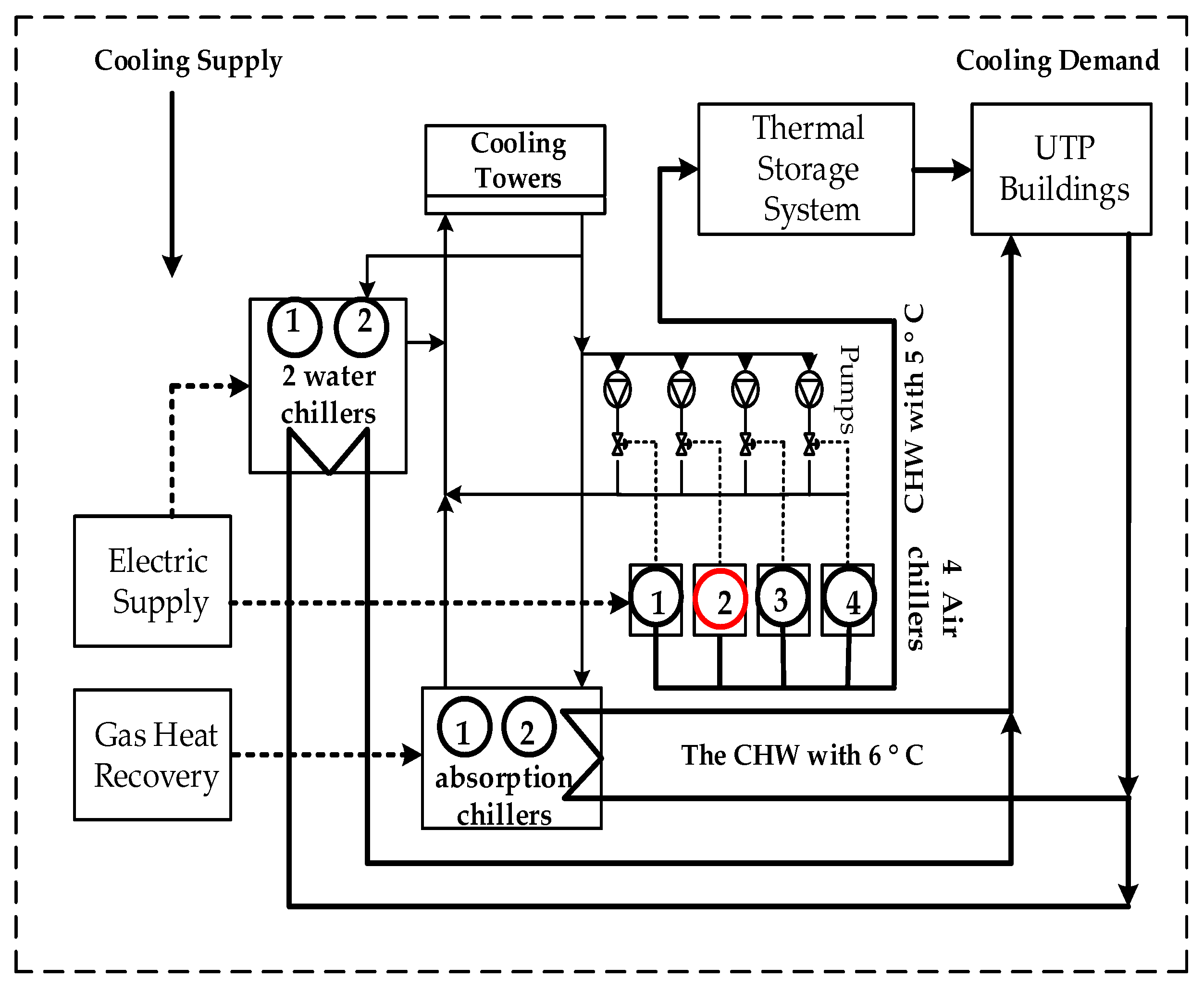
The DCS serving Universiti Teknologi PETRONAS was selected for investigation and is shown in Figure 1. It has eight chillers which are made up of two steam absorption chillers, two cooled water chillers, four cooled air chillers, and a thermal storage system.

The absorption and water chillers are used to send the chilled water (CHW) to consumers (buildings) directly. The four electric air chillers are operated to charge chilled water to the storage tank from 19:00 p.m. to 0.5:00 a.m. This CHW will be discharged from 06:00 a.m. to 20:00 p.m. to maintain the cooling demand requirements in UTP buildings [6]. Only 20 buildings are targeted for cooling by the DCS, while other buildings use small air-conditioning units. The targeted cooling buildings by DCS are: (1) Block 1 to Block 5 and Block 13 to Block 23 which are part of the academic building complex. It is used for staff offices, halls, labs, and student research. Each block is four floors high, (2) R&D Building: this is a four-floor research building with a total area of 21,225 square meters. It is used for carbon dioxide management and enhanced oil recovery research. It has 65 laboratories and accommodates up to 550 researchers, (3) Chancellor Complex which has a gross floor area of 40,000 square meters and is made up of the following: Chancellor Hall with capacity to accommodate 2910 persons; Resource Centre accommodating 2000 persons and over 500,000 books. It aims to provide up-to-date and adequate information resources to cater for the UTP population’s study and teaching needs, (d) Masjid An-Nur is a mosque, (4) Block C is a four floor building used for public and adjunct lectures. It also has some classrooms as well as the students’ health care center, and (5) Block D is an academic building consisting of four floors. It is made up of the student support unit, teaching, retail, and other student entertainment facilities. In this study, four Dunham Bush centrifugal chillers of the same capacities were used. Each of them has a rated cooling capacity of 325 Refrigerant Ton (1 RT = 3.517 kW). The total capacity of the chillers is stored in order to meet the demand during day-time hours. The chillers are connected in parallel and operate at constant speeds. The CHW pump consumes 15 kW to deliver the amount of CHW at 131 m³/h each. The CHW supply and return temperatures are 5 °C and 12.5 °C, respectively, when they operate at full load. The compressor power for each chiller is about 266.8 kW. The heat rejection in the chillers is attained with the aid of four cooling towers for each of the chillers. The towers have four cooling fans with a rated power of 16 kW each. This study is only concerned with one of these chillers (chiller No. 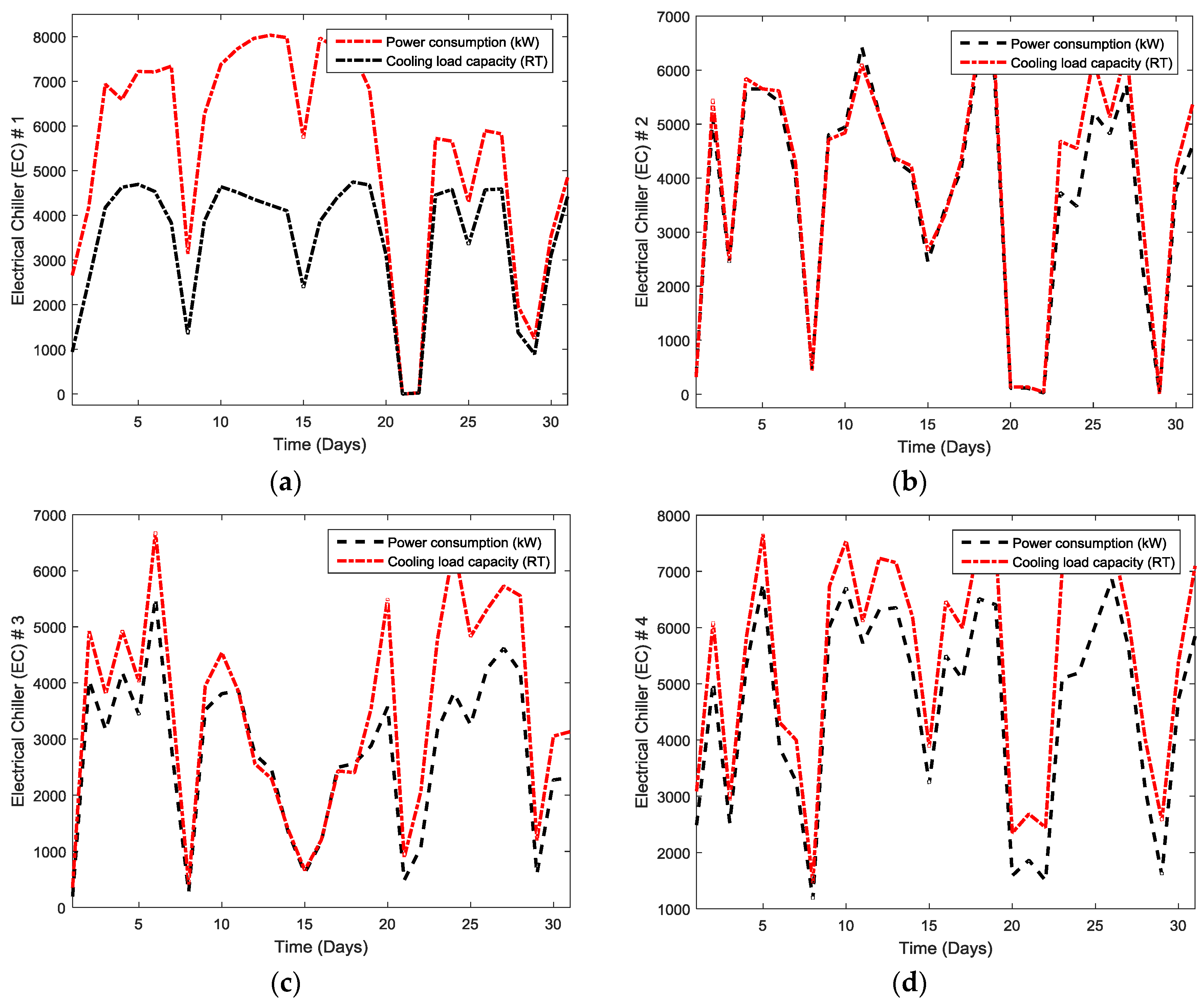2) as shown in Figure 2. The electrical chiller (EC) consumes a huge amount of energy, which resulted in lower efficiency and insufficient cooling. The study addressed this problem by proposing a novel method for re-evaluating the operating performance of the chiller (No. 2).

Table 1. The chiller recommended values.

Parameter	Value
COP (QkW/QC)	0.82
TCHWS/TCHWR (°C)	5/12.5
mCHW (kg/S)	36.68
∆TCHW (°C)	7.5
QC (RT)	325
QC (kW)	1143
Efficiency	4.28
QkW (kW)	266.8

shows the recommended values for each chiller, and Figure 2 shows power consumption and cooling load capacity for all four chillers system for the month of May 2016.

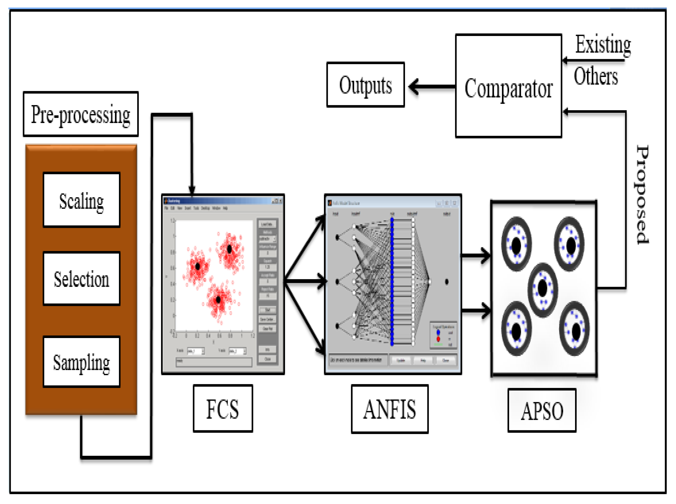
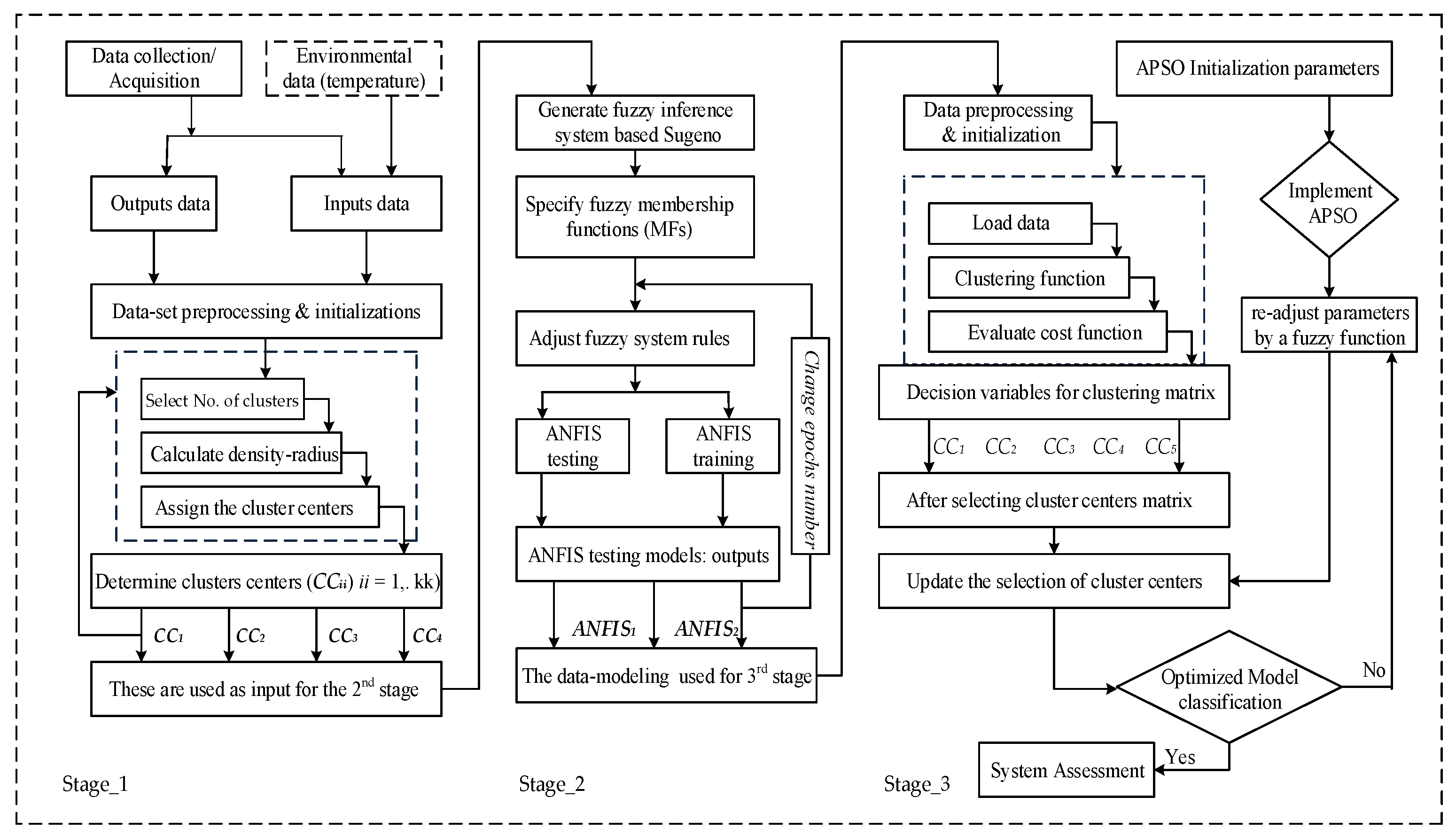
3. Proposed Methodology

Figure 3 shows the proposed methodology used to achieve the objectives of this work.

It can be implemented in four steps as follows:

(1) Data Preprocessing

The data was collected from the DCS. The data includes the variables flow rate of the CHW, supply and return temperatures of the CHW, number of chillers, operation load conditions, in addition to the ambient temperature. The variables were selected to fit the requirements of the clustering technique range between 0 and 1. The data were combined in two components-variables as stated in Section 3.1. Sampling was done on 744 data points and scaled to suit the clustering technique based on the FCS algorithm.

(2) Data Classification

The data collected in the Data Pre-processing stage were classified into grouping centers using the FCS algorithm to generate new fuzzy inference system (FIS) rules. The new extracted rules were used to determine the exact data-point centers to be used from the inputs and outputs data. A linear decision model based on fuzzy reasoning was introduced to tune the influence radius.

(3) ANFIS for Data Modeling

After classification of the data by the FCS algorithm, 5-layer ANFIS was applied to carry out the simulation process using two inputs, y_compI and y_compII. Thus, the data modeling output for estimating power consumption and cooling capacity is introduced for classification into five clusters.

(4) Data Classification and Optimization

The data modeling by ANFIS based on FCS is introduced through an objective function in the following section. This function is used to classify the data-set into five groups. Afterwards, APSO is employed to select the group or cluster center for data modeling and also to minimize the distance between data points and cluster center.

3.1. Basic System Modeling

The following section presents mathematical models based on statistical analysis for the collected real data of chillers plant to be represented by ANFIS. For k^th chiller (k = 1, 2,…, N), the operation mode γ_k can be expressed in two conditions as given in Equation (1):

$${\gamma }_k=\{\begin{array}{c}1, when k^{th} chiller is ON\hfill \\ 0, when k^{th} chiller is OFF\hfill \end{array}$$

(1)

In the chillers plant, the best performance occur, when the chiller’s compressor is operated at partial load (L_r). Thus, the chillers’ operation based on the input power to the compressor can be expressed by Equation (2) [38]:

$$Q_{kW}={\gamma }_k {\displaystyle \sum }_{k=1}^4(a_k+b_k{L}_r+c_k{L}_r^2+d_k{L}_r^3+e_k{L}_r^4)$$

(2)

where a_k, b_k, c_k, d_k, e_k are the power curve coefficients of k^th chiller. The chillers produce a mass flow of CHW (kg/s) at a supply temperature, T_CHWS via an evaporator for the distribution of load in order to serve the cooling utilities. The flow of CHW will return to enter evaporator under a certain return temperature, T_CHWR [1]. This chilled water must meet the requirements of cooling load demand in kW which can be expressed according to:

$$Q_C={\gamma }_k {\displaystyle \sum }_{k=1}^4{c}_p{m}_{CHW}\left(T_{CHWR}-T_{CHWS}\right)$$

(3)

where c_p is specific heat of CHW (4.197 kJ/kg °K), m_CHW is the flow rate of CHW in (kg/s), T_CHWR and T_CHWS are the return and supply temperatures of CHW in (°C), respectively. Therefore, the ratio of Equations (2) and (3) can be used to assess the operating chiller performance which is known as the coefficient of performance (COP). Thus, COP can be written as:

$$COP=Q_{kW}/Q_C$$

(4)

Thus, reducing power consumption will result in minimizing COP. Where the minimization of performance will result in increasing energy efficiency of chiller as given by Equation (5):

$$E{F}_{ici}=RT/COP$$

(5)

where EF_ici is the chiller efficiency, RT = 3.517 kW.

3.2. Data Modeling Preprocessing

The flow rate of CHW and its return/supply temperatures are two variables that will be affected by any increase/decrease in cooling load consumption [21,39,40,41,42]. However, energy efficiency will be affected by the increasing/decreasing cooling water return temperature, while reducing this temperature will result in an improved COP [43,44,45,46]. In this section the models to assess the COP for electric chillers will be predicted. The COP model will be developed according to the prediction of cooling load (Q_C) and power consumption (Q_kW). The behavior of Q_kW and Q_C can be simulated based on the selection of six influential variables: (1) the supply temperature of CHW (T_CHWS), (2) the return temperature of CHW (T_CHWR), (3) number of chillers (k), (4) the flow rate of CHW (m_CHW), (5) part load ratio (L_r), and (6) ambient temperature (T_amb). The T_amb is one of the influential variables that can be used as a climatic parameter [47]. This temperature, T_amb has effect on the temperature difference of CHW (∆T_CHW) that would result in an increase of cooling load consumption. Thus, ∆T_CHW is expressed in Equation as:

$$\Delta T_{CHW}=\left(T_{CHWR}-T_{CHWS}\right)$$

(6)

The recommended temperature of T_CHWS and T_CHWR are 5 °C and 12.5 °C, respectively. However, a T_CHWR reaches up to 19.3 °C due to the ambient temperature effect (θ) and this will result in more power consumption. Therefore, the return temperature of CHW can be expressed by Equation (7):

$${T^{\prime }}_{CHWR}=T_{CHWR}+\theta$$

(7)

$$\theta =\frac{2.5\lambda }{0.12}\underset{T_{amb,min}}{\overset{T_{amb,max}}{{\displaystyle \int }}}\frac{1}{T_{amb}}d{T}_{amb}+1.44$$

(8)

Herein, the T_amb for average values varies from 1 to 31 May 2016 [47]. Thus, the temperature, T’_CHWR can be expressed by Equation (9),

$${T^{\prime }}_{CHWR}=T_{CHWR}+\frac{2.5\lambda }{0.12}\underset{T_{amb,min}}{\overset{T_{amb,max}}{{\displaystyle \int }}}\frac{1}{T_{amb}}d{T}_{amb}+1.44$$

(9)

$$s.t; \lambda =\{\begin{array}{c}0, if T_{amb}<T_{amb,min}\hfill \\ \frac{T_{amb}-T_{amb,min}}{T_{amb,max}-T_{amb,min}},if T_{amb,min}\le T_{amb}\le T_{amb,max}\hfill \\ 1, if T_{amb}>T_{amb,max}\hfill \end{array}$$

(10)

Here by substituting Equations (9) and (10), the new temperature difference ∆T’_CHW according to T’_CHWR can be used as the first-component (y_compI) to assess the cooling load which can be expressed by:

$$y_{compI}=\Delta T{\prime }_{CHW}={T^{\prime }}_{CHWR}-T_{CHWS}$$

(11)

Also, the flow rate of chilled-water (m_CHW) is of factors can influence power consumption. However, during the off-peak hour, a number of chillers (k) are operated under partial load (L_r) conditions. Thus, the second-component can be written as,

$$y_{compII}=k{m}_{CHW}{L}_r$$

(12)

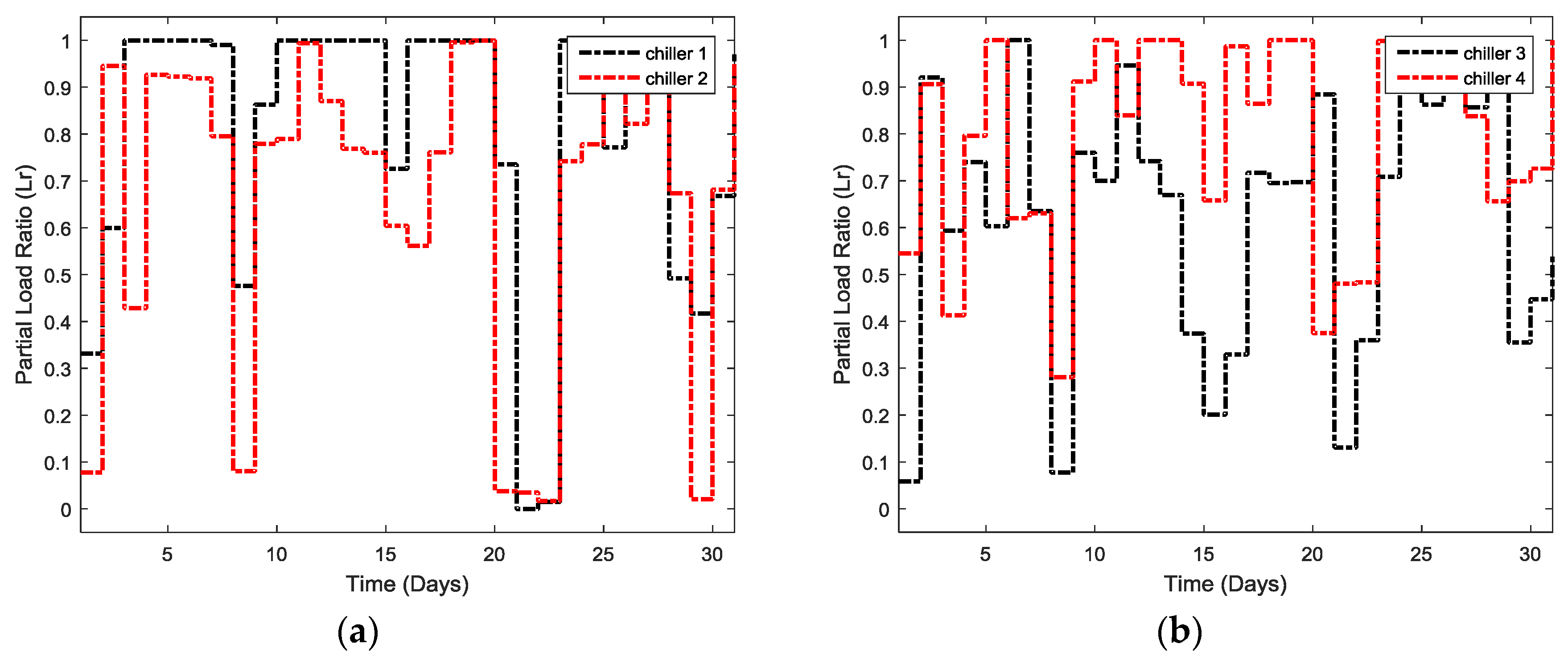
Equations (11) and (12) are used to predict the power consumption and cooling load capacity by Equations (2) and (3). Then, it will be used to assess the COP based on data classification of energy consumption and cooling load. In this work, chiller 2 is adopted for assessment and it will be operated under partial load condition. Figure 4 shows the operating conditions of all four chillers including chiller 2.

3.3. Fuzzy Clustering Subractive

A fuzzy clustering subtractive (FCS) algorithm is used to estimate the data clustering numbers. In particular, the data will be scaled between (0, 1) and each data sampling point will be assigned as a potential cluster center. The cluster centers are calculated and l^th data points or grouping (u_l = u₁, u₂, u_z) have high influences on any cluster center within this group. Assume M dimensions, the density function D_l of l^th data point is expressed by:

$$D_l={\displaystyle \sum }_{l=1}^{z}exp\left\{\frac{{\Vert u_l-u_p\Vert }^2}{{\left(r_a/2\right)}^2}\right\}$$

(13)

where u_l and u_p are data points, r_a is the influence radius. The 1st cluster center will be at the highest density point u_CCl. In the next cluster center, the density of each u_l data point is expressed by:

$$D_l=D_l-D_{C{C}_l}{\displaystyle \sum }_{l=1}^{z}exp\left\{\frac{{\Vert u_l-u_p\Vert }^2}{{\left(r_a/2\right)}^2}\right\}$$

(14)

From Equation (14), the distance between data point u_l and cluster center u_p can be written as:

$$d_{lp}=exp\left\{-\frac{{\Vert u_l-u_p\Vert }^2}{{\sigma }^2}\right\}$$

(15)

The membership function μ_l for lp^th each cluster of data-point can be computed by [48]:

$${\mu }_l=exp\left\{-{\displaystyle \sum }_{p=1}^M\frac{-{\left(u_{lp}-c_{tr}\right)}^2}{2{\sigma }_p^2}\right\}$$

(16)

where u_lp is the corresponding data points, c_tr is the cluster center, $\sigma$ = $\sqrt{\alpha }$/2 and α = 4/$r_a^2$ [49]. The influence radius, r_a is sufficient for most studies with acceptable results ranged 0.1 to 0.7 [48,50]. A lower r_a generates more clusters, these clusters be closer to each other and this would result in less errors. High r_a should be used in a low density data, which will result in a small number of clusters, in this particular case, a fuzzy model is introduced with a fuzzy decision function of r_a by:

$$r_a=\left\{\begin{array}{cc}1,& when f_a\le f_a^{min}\\ \frac{f_a-f_a^{min}}{f_a^{max}-f_a^{min}},& when f_a^{min}<f_a<f_a^{max}\\ 0,& when f_a\ge f_a^{max}\end{array}\right\}$$

(17)

where $f_a^{min}$ and $f_a^{max}$ are the minimum and maximum values of a^th objective function. If r_a = 0, it will be only one cluster (the first) and hence no more clusters after the first one. If r_a = 1, the numbers of clusters generated will be few and best (r_a) to be ranged $f_a^{min}<f_a<$ $f_a^{max}$ according to Equation (17).

3.4. Adaptive Neuro-Fuzzy Inference System

The Adaptive Neuro-Fuzzy Inference System (ANFIS) is a logic controller introduced in 1993 by Jang et al. [35]. It is a combination of an artificial neural network (ANN) and fuzzy inference system (FIS). The ANN and FIS have good capabilities and interpretability for learning methods and both are used as expert systems [31]. The combination of these two techniques overcome the limitations of ANN computational time and FIS rules error [27,28,29,30,31].

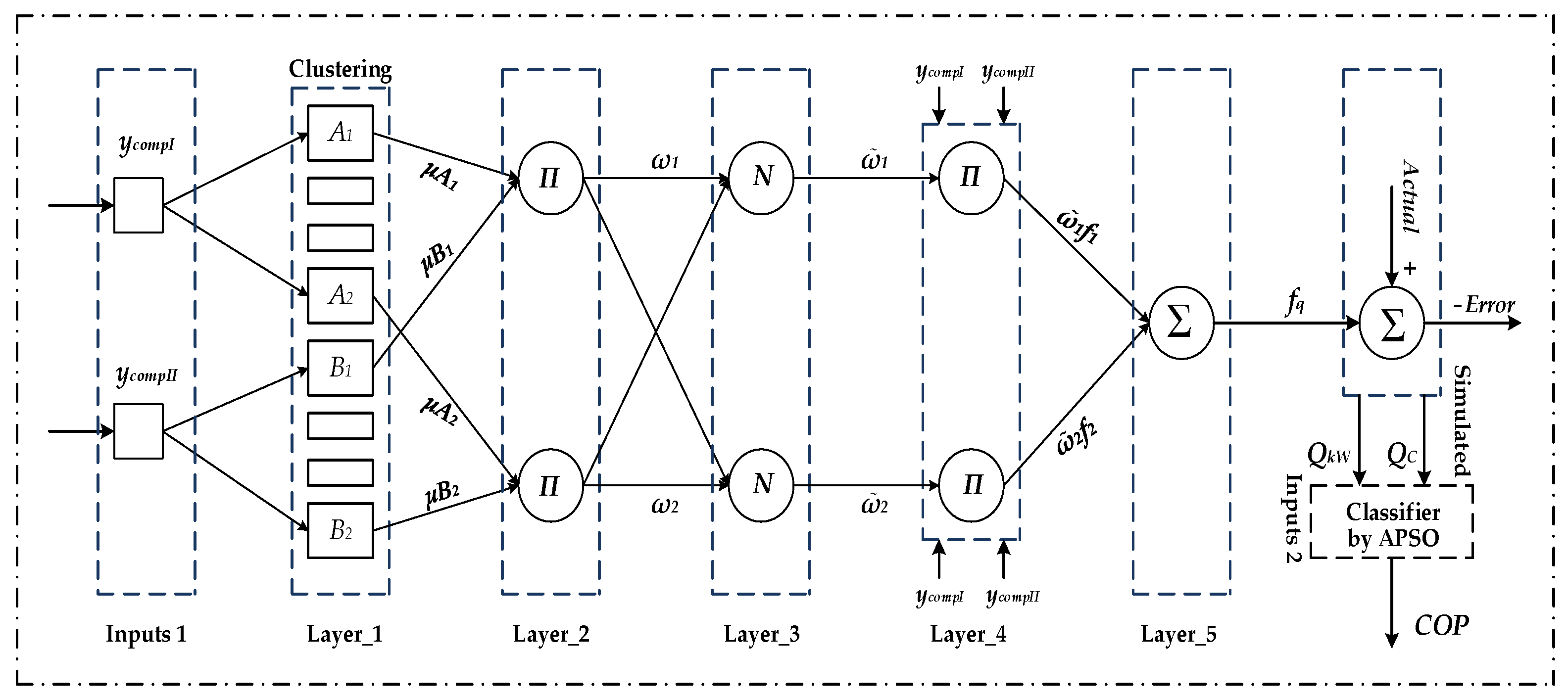
In this work, two models will be predicted, which are cooling load capacity (Q_C) and power consumption (Q_kW) to assess the chiller performance. The two models have two inputs, y_compI and y_compII in the ANFIS structure shown in Figure 5.

Then, a Sugeno fuzzy inference system (Sugeno-FIS) is used to generate the system rules from the input variables to the outputs. The combination of inputs can be modeled as first order using “fuzzy if-then rules” by:

$$Rule\#1=if \left(y_{compI} is A_1\right) and \left(y_{compII} is B_1\right), then f_1=m_1{y}_{compI}+n_1{y}_{compII}+o_1$$

(18)

$$Rule\#2=if \left(y_{compI} is A_2\right) and \left(y_{compII} is B_2\right), then f_2=m_2{y}_{compI}+n_2{y}_{compII}+o_2$$

(19)

where y_compI and y_compII are the input variables, A_q and B_q are the fuzzy sets of antecedents, f_q are the system outputs, and m_q, n_q, o_q are the parameters of fuzzy consequences. The structure of ANFIS shown in Figure 5 has five layers, each layer with specific task.

In Layer 1, each node gives a function, and the output of the q^th node in each m^th layer is denoted by $D_q^m$, then this function can be expressed by:

$$D_q^1=\mu A_q\left(y_{compI}\right), when q=1, 2$$

(20)

$$D_q^1=\mu B_{q-2}\left(y_{compII}\right), when q=3, 4$$

(21)

Let A = (A₁, A₂, B₁, or B₂), therefore each q generates membership grades of input variables with the Gaussian function. The output of the q^th node in the Layer 1 based on FCS in Equation (16) is given by Equation (22):

$$D_q^1=\mu A_q\left(y_{compI}\right)=\exp {\left\{\frac{-\left(y_{compI}-c_q\right)}{2{\sigma }_q^2}\right\}}^2$$

(22)

where μA_q is the corresponding membership function, y_compI or y_compII are the input to the node at Layer 1, σ_q and c_q are parameters sets of membership functions (MF) determined from the actual data. When the parameters change, the MF shape changes accordingly. In Layer 2, each q in this layer is a fixed node labelled and then the output is the multiplication of labeled data as expressed by Equation (23):

$$D_q^2={\omega }_q=\mu A_q\left(y_{compI}\right)\times \mu B_q\left(y_{compII}\right), q=1, 2$$

(23)

In Layer 3, the q will be calculated as the ratio of the firing strength to the total of all firing strengths using Equation (24):

$$D_q^3={ῶ}_q=\frac{{\omega }_q}{{\omega }_1+{\omega }_2},q=1, 2$$

(24)

In Layer 4, the output in Equation (24) will be multiplied by the first order model in Equations (18) and (19), where it represents the weights (ῶ_q) of the consequent of each calculated fuzzy rule. The overall output is given in Equation (25):

$$D_q^4={ῶ}_q\times f_q={ῶ}_q\left(m_q{y}_{compI}+n_q{y}_{compII}+o_q\right)$$

(25)

In Layer 5, the summation in Layer 4 will be calculated in this node as weighted, therefore the overall output can be written as,

$$D_q^5={\displaystyle \sum }_q{ῶ}_q{f}_q=\frac{{{\displaystyle \sum }}_q{\omega }_q{f}_q}{{{\displaystyle \sum }}_q{\omega }_q}$$

(26)

The ANFIS algorithm is a hybrid of gradient descent and least squares methods. When the premised parameters are fixed, the final output for each model is a linear combination of the consequent parameters. Based on the 2 variable-components y_compI and y_compII, the overall output for each model (f_q = f₁ + f₂) can be expressed in Equation (27) as:

$$f_q=f_1+f_2=\frac{{\omega }_1\times m_1{y}_{compI}+{\omega }_1\times n_1{y}_{compII}+{\omega }_1\times o_1}{{\omega }_1+{\omega }_2}+\frac{{\omega }_2\times m_2{y}_{compI}+{\omega }_2\times n_2{y}_{compII}+{\omega }_2\times o_2}{{\omega }_1+{\omega }_2}$$

(27)

3.5. ANFIS-Based FCS and ANFIS-Based FCM Set-Up

Three techniques have been developed: (1) ANFIS-based FCS, (2) ANFIS-based fuzzy clustering-means (FCM), and (3) the traditional ANFIS. The techniques were developed and executed in two parts: training and checking of the data. 75% (588) of the data sampling points were used as training data selected randomly from the recoding, whereas the remaining 25% (186) of the data sampling points were used as testing data to verify the ANFIS models. The data was simulated in MATLAB Environment. From the data collected (1–31 May 2016), the Q_kW and Qc are 122,495 kWh and 115,174 RTh, respectively (COP = 1.06, Equation (4)). Therefore, the chiller did not perform efficiently. Here, ANFIS-based FCS and ANFIS-based FCM data modeling were developed and compared with the ANFIS.

Table 2. ANFIS-based Fuzzy Clustering Subtractive parameter for Chiller 2.

ANFIS-Based FCS: Chiller 2	QkW	QC
No. of nodes	29	29
No. of linear parameters	12	12
No. of non-linear parameters	16	16
Total No. of parameters	28	28
No. of training data pairs	558	558
No. of checking data pairs	186	186
No. of each input (ycompI&II)	2	2
No. of fuzzy rules	4	4
No. of clusters	4	4
No. of epoch	250	250
Influence radius (ra)	0.12	0.12
Error goal	0	0
Initial step size	0.01	0.01
Step size decrease rate	0.9	0.9
Step size increase rate	1.1	1.1

and

Table 3. ANFIS-based Fuzzy C-Means clustering parameter for Chiller 2.

ANFIS-Based FCM: Chiller 2	QkW	QC
No. of nodes	29	29
No. of linear parameters	12	12
No. of non-linear parameters	16	16
Total No. of parameters	28	28
No. of training data pairs	558	558
No. of checking data pairs	186	186
No. of each input (ycompI&II)	2	2
No. of fuzzy rules	4	4
No. of clusters	4	4
No. of epoch & iterations	250	250
Minmum improvement	0.00001	0.00001
Error goal	0	0
Initial step size	0.01	0.01
Step size decrease rate	0.9	0.9
Step size increase rate	1.1	1.1
Partition matrix exponent	2	2

show simulation parameters for the data-set of Q_kW and Q_C versus y_compI & y_compII.

3.6. System Classifier-Based Optimization Method

To reassess the operating performance of Chiller 2, the power consumption and cooling capacity data was analyzed with the aid of the ANFIS-based FCS and computed using:

$$f_{Q_{kW}}=7.3674y_{compI}+7.3674y_{compII}+8.9967$$

(28)

$$f_{Q_C}=8.9967y_{compI}+8.9967y_{compII}+9.9967$$

(29)

Equations (28) and (29) are objective functions which need to be minimized and can be written as Equation (30) with constrained values for variables of y_compI and y_compII in Equation (31):

$$f_{q\left(g_g\right)}\downarrow =COP=min \left\{\frac{f_{Q_{kW}}}{f_{Q_C}}\right\}$$

(30)

$$g_g=\left\{\begin{array}{c}0\le k\le 1\\ 0.1\le l_r\le 1\\ 0\le \theta \le 6.8\\ 0.1\le \lambda \le 1\\ 5\le T_{CHWS}\le 5.5\\ 12.5\le {T^{\prime }}_{CHWR}\le 19.8\\ 0\le m_{CHW}\le 36.68\\ 26.4\le T_{amb}\le 34\end{array}\right\}$$

(31)

3.6.1. PSO Algorithm

PSO was first used to simulate the foraging swarm of particles such as bird flocks and fish schools by Kennedy and Eberhart [51]. Each particle (i) is defined by its position x_ij^t = {x_i1^t, x_i2^t,…, x_ij^t,…, x_im^t} and velocity v_ij^t = {v_i1^t, v_i2^t,…, v_ij^t,…, v_im^t} of j^th dimension. At each iteration, i remembers the best position achieved so far and stores it as (pbest_ij^t). Then each i stores the best position achieved in the whole swarm as (gbest_j^t). At each step, a particle is directed to fly a distance with a velocity, defined as a weighted term with separate random numbers toward a location of pbest and gbest. Hence, the velocity of particles and their positions can be expressed by [1]:

$$v_{ij}^{\left(t+1\right)}=ck\left\{w{v}_{ij}^{\left(t\right)}+c_{1}r{1}_{ij}\left(pbes{t}_{ij}^{\left(t\right)}-x_{ij}^{\left(t\right)}\right)+c_{2}r{2}_{ij}\left(gbes{t}_j^{\left(t\right)}-x_{ij}^{\left(t\right)}\right)\right\}$$

(32)

$$x_{ij}^{\left(t+1\right)}=x_{ij}^{\left(t\right)}+v_{ij}^{\left(t+1\right)}, i=1, 2,\dots , ps \left(particles\right)$$

(33)

where v_ij^t+1 is the updated velocity for the particles at iteration (t + 1), and v_ij is the velocity of i^th particle at iteration, t,. Where the velocity can be expressed by this boundary:

$$v_{ij,min}\le v_{ij}\le v_{ij,max}$$

(34)

c₁ and c₂ are the learning factors used to accelerate particles to find pbest_ij^t and gbest_j^t, and r₁, r₂ are random numbers (0, 1) with a matrix dimension (ij), x_ij^t+1 is the updated particle’s current position, ck is the constriction factor and w is the inertia weight expressed as:

$$w=w_{max}-\left[\frac{w_{max}-w_{min}}{I{t}_{max}}\right]iter$$

(35)

$$ck=2\ast \zeta /\left\{\left|2-{\psi }_{ij}-\sqrt{\left|{\psi }^2-4\psi \right|}\right|\right\}$$

(36)

where w_max and w_min are initial and final inertia weight factors, respectively, iter is the current iteration number, It_max is the maximum iteration, and ζ is a constant = 1. Herein, it is known that PSO has a shortcoming which is converging at high speed [36,37], to avoid this drawback, an accelerated PSO (APSO) based fuzzy is proposed in Section 3.6.2. Even though, PSO was used to solve the objective function in Equation (30).

Table 4. The setting parameters of Particle Swarm Optimization.

Symbol	Value	Symbol	Value
Swarm	50	wmax	0.95
Itmax	250	vmax	+0.5 *v
c1	1.5	vmin	−0.5 *v
c2	1.5	r1, r2	0, 1
wmin	0.35	ck	0.733

lists the parameters of PSO that have been used in this study.

3.6.2. Accelerated Particle Swarm Optimization

To accelerate the convergence of PSO, an accelerated particle swarm optimization (APSO) is used [52]. The APSO could accelerate the convergence using the global best only. Therefore, the updated particle’s velocity and its position can be modified by:

$$v_{ij}^{\left(t+1\right)}=v_{ij}^{\left(t\right)}+\alpha r_{ij}+\beta \left(gbes{t}_j^{\left(t\right)}-x_{ij}^{\left(t\right)}\right)$$

(37)

$$x_{ij}^{\left(t+1\right)}=x_{ij}^{\left(t\right)}\left(1-\beta \right)+\beta \left(gbes{t}_j^{\left(t\right)}\right)+\alpha r_{ij}$$

(38)

where r_ij is a random number (0, 1), α and β are parameters typically less than 1. In most applications, it uses β = 0.1~0.7 and α = 0.1~0.5 [52], whereas, in other studies the values ranged between α = 0.1~0.4 and β = 0.1~0.7 [53]. In this study, it is recommended to set α = 0.2 and β = 0.5. However, β can be adjusted using a fuzzy linear model by:

$${\beta }_i^t=\left\{\begin{array}{cc}1,& when y_i\le y_i^{min}\\ \frac{y_i-y_i^{min}}{y_i^{max}-y_i^{min}},& when y_i^{min}<y_i<y_i^{max}\\ 0,& when y_i\ge y_i^{max}\end{array}\right\}$$

(39)

where $y_i^{min}$ and $y_i^{max}$ are the minimum and maximum values (0~1) (ob). If β = 0, there will be no movement for the particle, i, no updating for the velocity and the particle will be fixed at only one position. If β = 1, there will be no change in the global best and no updating in the current position. Thus, the fuzzy decision for β ranged between (0.1~0.7) at t population. The membership’s degree can be determined by:

$${\beta }^t=\frac{{{\displaystyle \sum }}_{i=1}{\beta }_i^t}{{{\displaystyle \sum }}_{t=1}{{\displaystyle \sum }}_{i=1}{\beta }_i^t}$$

(40)

To solve objectives functions in Equation (30), APSO was used and

Table 5. The setting parameters of Accelerated Particle Swarm Optimization.

Symbol	Value	Symbol	Value
Swarm	50	nD	2
Itmax	250	vmax	+0.5 *v
α	0.47	vmin	−0.5 *v
β	0.63	rij	0, 1

shows their parameters for power consumption and cooling capacity optimization.

3.7. Methodology Implementation

The study was implemented in three steps as mentioned earlier, and the procedures for the steps are as follows:

• In the 1st step, the data collected for T_CHWS, T_CHWR, m_CHW, T_amb, L_r, and k were selected and scaled to be clustered by FCS algorithm.
• Each of these data was classified into five groups of l^th data (u_l = u₁, u₂,…, u₅) using FCS algorithm.
• Each group or cluster has a center or mean represented by the vector of p^th (u_p = u₁, u₂,…, u₅).
• The data density D_l was calculated to determine data grouping with their 5 centers using Equation (13).
• In density formula, the radius of cluster or influence radius was adapted by a fuzzy linear function in Equation (17) for an appropriate number for the clusters.
• In the 2nd step, the data was loaded and simulated into two parts; training data model and testing data model.
• 75% of the collected data was employed for training data, whereas 25% was used to verify the model.
• A matrix relationship for input data—output data was created.
• The training data was used to build fuzzy membership function using Gaussian with 2-4-4.
• The 2-4-4 are 2 ANFIS-based FCS inputs (y_compI and y_compII), 4 memberships function, and 4 Sugeno FIS rules.
• Each input based FCS has 4 values and the all memberships function inputs responsible for determining/developing the final output model of first order model based Sugeno FIS.
• The training data used a hybrid learning algorithm to identify consequent parameters of each model.
• The model fitness performance for training/testing data occurred when both reach to a minimum and similar error.
• In the 3rd step, the output data of ANFIS-based FCS was loaded, clustered again and then optimized by APSO.
• The variables in Equations (28) and (29) were defined and ranged in Equation (31) and then optimized based a classifier in Equation (30).
• Then data loaded in two input columns.
• The clustering cost function was created based on numbers of decision variables.
• A decision matrix clustering was created in five positions for each input column.
• Calculate the density and identify the cluster centers with adjustable cluster radius.
• Then, the velocity of particles and their position were initialized.
• The clustering cost function was evaluated.
• The global best position for the particles was selected for assigning cluster centers.
• The velocity limits for the particles were initialized and applied.
• Then, the velocity of particles was updated.
• The system output was evaluated, otherwise APSO parameters re-adjusted by the fuzzy system.

The implemented parameters for ANFIS-based FCS and APSO are given in Table 2 and Table 5, and Figure 6 shows the implementation of the ANFIS-based FCS with the APSO flow chart.

4. Results and Discussion (Part 1)

4.1. ANFIS-Based FCS and ANFIS-Based FCM Set-Up

ANFIS were developed and executed in two parts; training and checking data. 75% of data sampling points were used as training data selected randomly from the recording, while the remaining 25% were used as testing data to verify the ANFIS models. The system has been implemented in a MATLAB environment based on the actual data that have been collected during the period (1–31 May 2016). From that, the power consumption and cooling load capacity of a chiller 2 were 122,495 kWh and 115,174 RTh, respectively. Based on actual data, the estimated COP is 1.06, which is less efficient compared to other chillers shown in Figure 2. In this study, the simulation was implemented on two models (Q_kW and Q_C) against variables of the two-component y_compI and y_compII.

4.1.1. ANFIS-Based FCS Technique

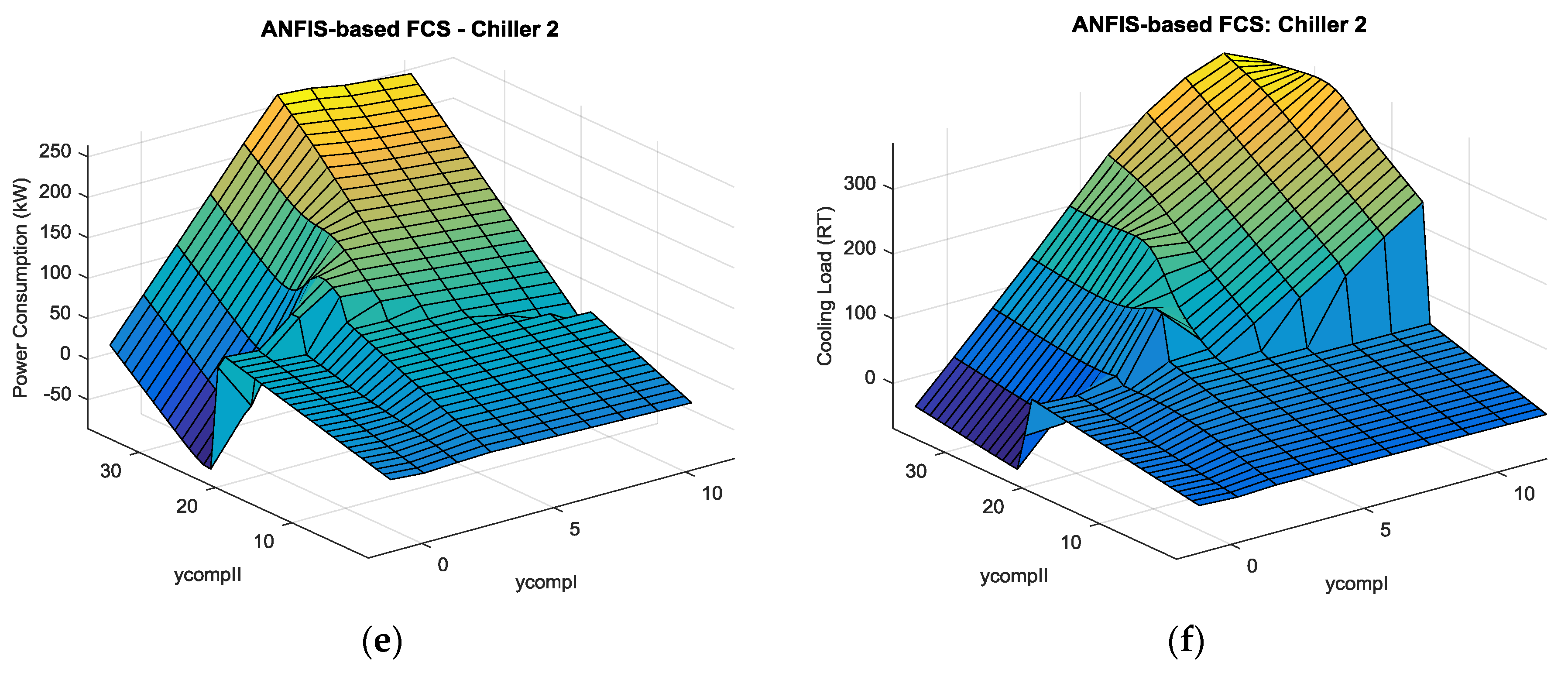
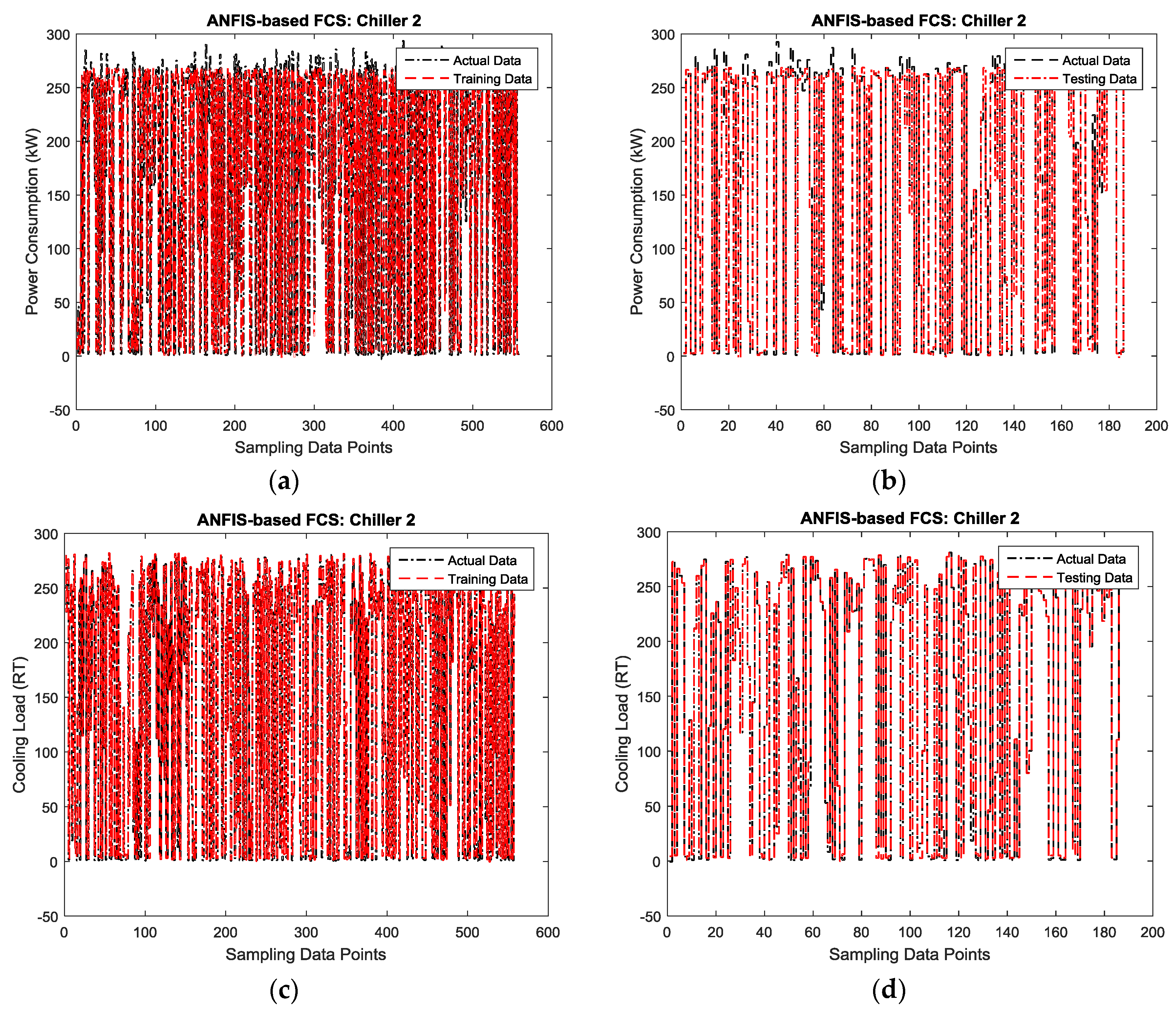
The results obtained for the ANFIS-based FCS are shown in Figure 7. The results indicate that the training and testing data for power consumption and cooling load were identically consistent with the actual data in Figure 7a–d, respectively. The power consumption and cooling load models are shown in a surface plot output versus two input variables, y_compI and y_compII in Figure 7e,f, respectively. The actual data for the power consumption in Figure 7b is identical with the simulated power with a mean error of 1.62% (0.02).

Meanwhile, the predictive cooling load capacity is also identical in Figure 7d. Therefore, the simulation of predictive power consumption and cooling load capacity are almost similar to the existing system. The analytical performance for the simulation using ANFIS-based FCS according to the coefficient of determination (R²), it was about 0.99601 and 0.99895 for power consumption and cooling capacity, respectively. Hence, the simulation results tend to be similar to the existing DCS system at UTP.

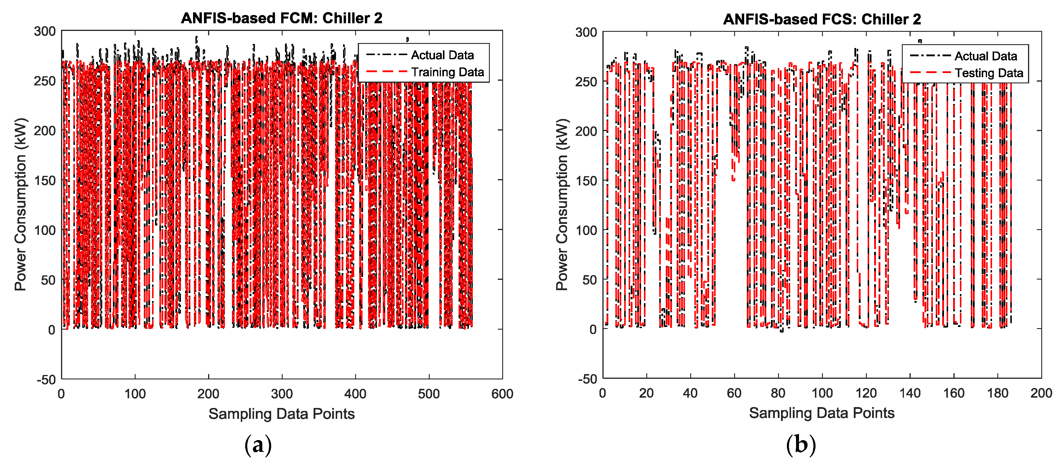
4.1.2. ANFIS-Based FCM Technique

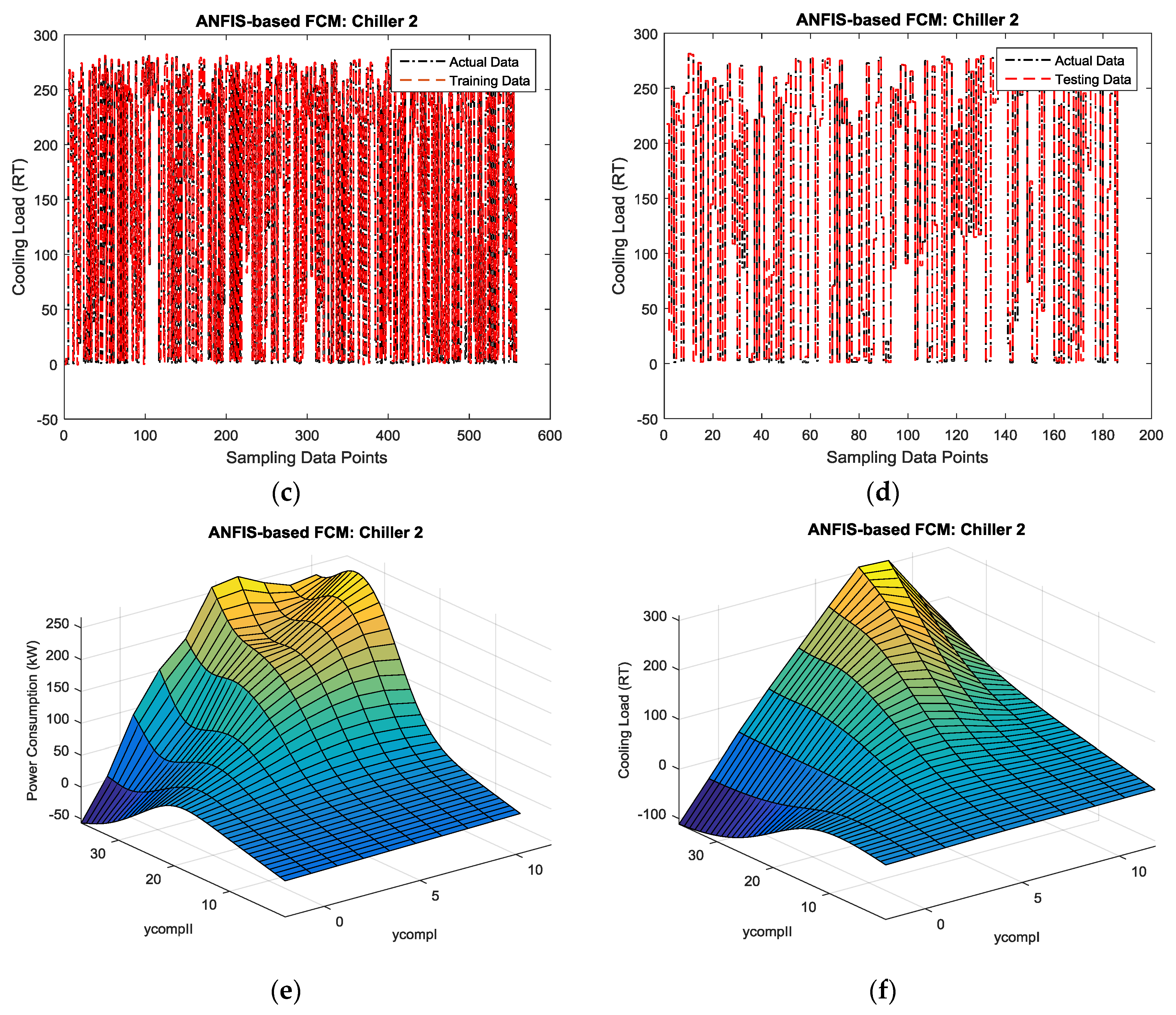
The ANFIS-based FCM model was implemented and simulated, and the results are given in Figure 8. The results indicate that the training and testing data for power consumption and cooling load were also identically consistent with the actual data as in Figure 8a–d, respectively. The data for power consumption and cooling load models are shown in a surface plot of output versus two input variables, y_compI and y_compII (Figure 8e,f, respectively).

The actual energy consumption in Figure 8d was compared with the one simulated using ANFIS-based FCM and the cooling load capacity in Figure 8f was also compared with the simulated too. Herein, the simulation performance was not similar to the actual data in case of ANFIS-based FCM. The regression for both power consumption and cooling load capacity are 0.99436 and 0.99825, respectively. This resulted in increases in root square mean error (RSME) as given in

Table 6. A comparison between ANFIS-based FCS and ANFIS-based FCM.

Model Performance	RMSE (QkW)	RMSE (QC)	R2 (QkW)	R2 (QC)
ANFIS-FCS: Training data	12.3570	5.3446	0.99440	0.99890
ANFIS-FCS: Testing data	11.2486	5.3264	0.99601	0.99895
ANFIS-FCM: Training data	12.2018	5.7747	0.99460	0.99873
ANFIS-FCM: Testing data	12.6965	6.8174	0.99434	0.99825

for both ANFIS-based FCS and ANFIS-based FCM. Therefore, the analytical data based on R² and RSME show that the ANFIS-based FCS is more accurate compared to the ANFIS-based FCM.

5. Results and Discussion (Part 2)

The objective function in Equation (30) was introduced and the COP was optimized based on the APSO. The COP was optimized using data classification for Q_kW and Q_C. The data for Q_kW and Q_C were classified and assign cluster centers with a density minimization by:

$$D_l=min{\displaystyle \sum }_{l=1}^{z}exp\left\{\frac{{\Vert u_l-u_p\Vert }^2}{{\left(r_a/2\right)}^2}\right\}$$

(41)

Herein, a fuzzy adopts to partitioning system with membership ranges between 0 and 1. Five clusters (u_p, p = 1, 2, 3, 4, 5) were grouped using the APSO algorithm from the output data of the ANFIS-based FCS. For u_l = 1, 2 the data pairs for cluster Q_kW and Q_C can be written as (Q_kW1, Q_kW2, Q_kW3, Q_kW4, Q_kW5) and (Q_C1, Q_C2, Q_C3, Q_C4, Q_C5). The clusters u_p were assigned five centers for each cluster of Q_kW and Q_C. The data were scaled by 300 to satisfy clustering dimensions (0, 1). Each particle i has j dimensions j = 1, 2 to indicate the set-point value for each particle vector. This j^th particle vector in the search space is restricted according to the specific scaling. After data has been classified by PSO and APSO, the data was multiplied by 300 (re-scaled) again to give the final classification based on five cluster centers.

5.1. Classifier-Based PSO

After the fuzzy algorithm was adopted to the partitioning system with membership ranging from (0~1), the matrix obtained for cluster centers using PSO is given by:

$$PSO=\left\{\begin{array}{c}Cluster center 1\\ Cluster center 2\\ Cluster center 3\\ Cluster center 4\\ Cluster center 5\end{array}\right\}=\left\{\begin{array}{cc}47.1446& 45.9117\\ 01.6115& 01.9193\\ 184.0488& 195.7765\\ 269.5352& 262.7565\\ 110.9093& 146.9420\end{array}\right\}=\left\{\begin{array}{c}1.0268\\ 0.8396\\ 0.9401\\ 1.0258\\ 0.7548\end{array}\right\}$$

(42)

where each row in the matrix represents cluster centers, while the first and second column represent power consumption and cooling load capacity, respectively. The last column represents COP. In cluster 1, the chiller was operated at a condition of the partial load (18%). The power consumption and cooling load capacity were 47.1446 kW and 45.9117 RT, respectively and this resulted in a COP of 1.0268. In cluster 2, the chiller was not operated at a condition of no load (0%), while in cluster 3, the chiller was operated at a condition of (69%) and its operating performance COP was 0.9401. In cluster 4, the chiller was operated at a condition of the full load (100%). Where it consumed a power of 269.5 kW and delivered a cooling capacity of 262.7 RT. In this case, the chiller performed efficiently with a COP of 0.9401, which is even better than the existing system. In cluster 5, the chiller operated at a condition of the partial load (42%) and performed efficiently with COP of 0.7548. Therefore, overall performance for cluster 1 and cluster 4 shows that the chiller performed well compared to the existing system. Based on the recommended values, the chiller did not perform efficiently. This is because of several influential factors mentioned earlier. The chiller energy efficiency according to Equation (5) is about 3.4252 and 3.4288 for cluster 1 and cluster 4, respectively. For clusters 3, the chiller performance improved a little bit compared to clusters 1 and 4. In the 5th cluster, the chiller was operated and performed more efficiently than the recommended values. Cluster 5 represents efficient cluster for the chiller and power consumed. The overall operating performance using PSO-based classifier was optimized and gave COP of 0.9393 with an efficiency of 3.74.

5.2. Classifier Based APSO

After fuzzy was adopted to partitioning system with membership ranged (0~1), the matrix of clusters obtained after performing APSO are:

$$APSO=\left\{\begin{array}{c}Cluster center 1\\ Cluster center 2\\ Cluster center 3\\ Cluster center 4\\ Cluster center 5\end{array}\right\}=\left\{\begin{array}{cc}255.5098& 270.5731\\ 184.0491& 195.7763\\ 1.8728& 2.2026\\ 273.3892& 260.5466\\ 110.1508& 146.0347\end{array}\right\}=\left\{\begin{array}{c}0.9443\\ 0.9401\\ 0.8503\\ 1.0493\\ 0.7543\end{array}\right\}$$

(43)

Five clusters have been assigned for paired data of power consumption and cooling capacity using APSO. In cluster 1, it consumed 255.5 kW power and produced a cooling capacity of 270.5 RT.

The energy efficiency in this cluster increased by 3.7245 and the COP improved by 0.9443 compared to that using PSO. In cluster 2, the chiller consumed 184.5 kW and produced 195.8 ton. The COP is 0.9401, which is similar to that of cluster 3 in PSO. In the 4th cluster, APSO consumed about 273.5 kW, which is even more than the rated value (266.8 kW) with a production of 260.5 RT cooling capacity. In this particular case, the chiller did not perform efficiently. Therefore, energy efficiency in this case is about 3.3518 which is even less than PSO. Cluster 5 is one of the most efficient clusters with a 0.7543 improvement in COP and energy efficiency increase 4.6626. In this case, COP and EF_ici were even better than the recommended. The overall operating performance using PSO-based classifier was optimized to give COP of 0.8908 with an efficiency of 3.95. It can be concluded that APSO demonstrated that it is an efficient tool for data classification compared to PSO. Also, it outperformed PSO drawback regarding the problem of convergence. 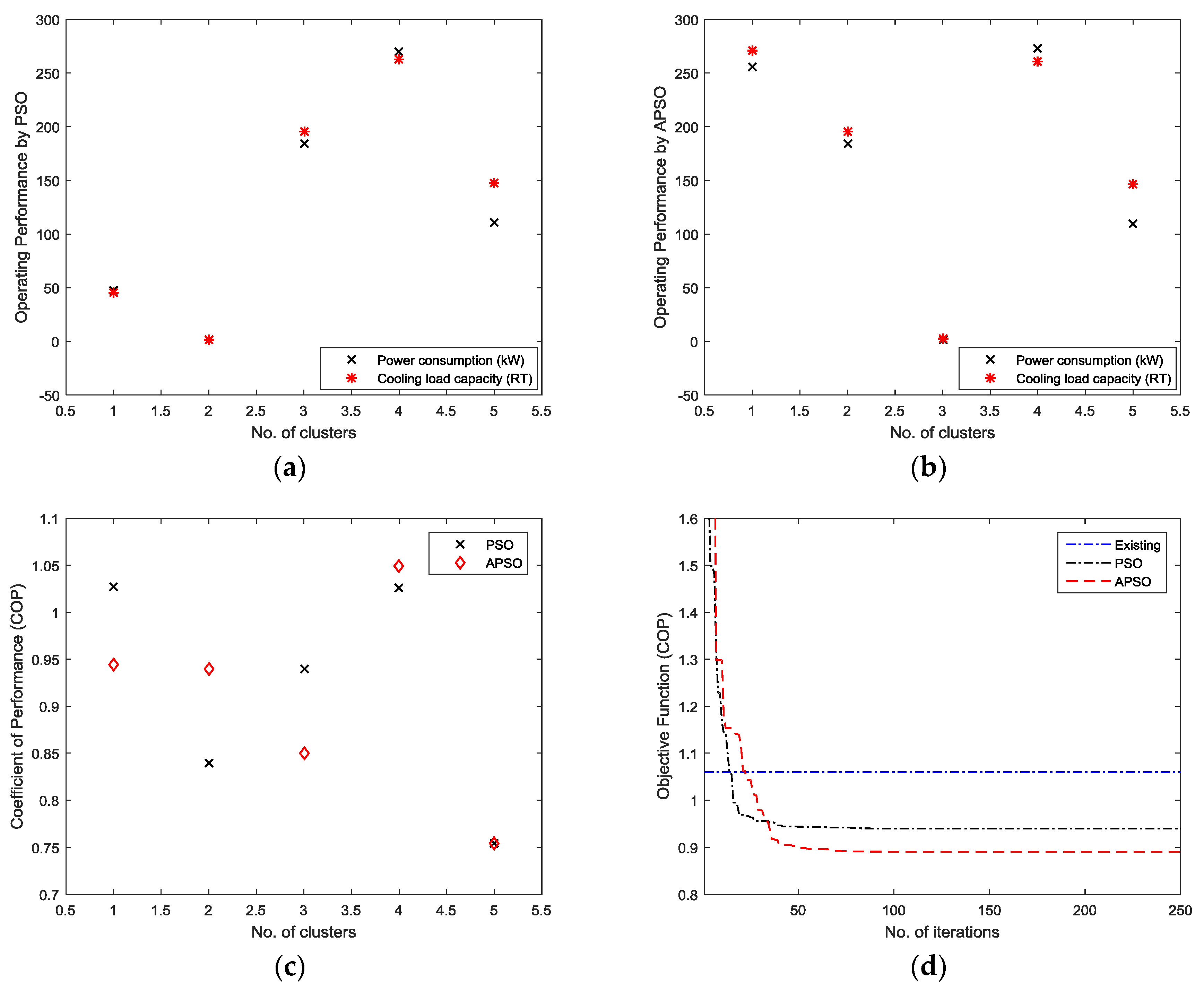Figure 9a,b shows the final classification for five cluster centers by PSO and APSO, respectively. Figure 9c shows the clustering of COP based on calculation of (a) and (b). Figure 9d shows the objective function using PSO and APSO compared to the existing system.

The energy efficiency of the chiller increased when the ANFIS-based FCS classified with APSO was used compared to when the ANFIS-based FCS classified with PSO as shown in

Table 7. A comparison of chiller efficiency.

Cluster	EFici (Exsiting)	EFici (PSO)	EFici (APSO)	Increased (PSO)%	Increased (APSO)%
Cluster#1	3.3179	3.4252	3.7245	3.23	12.25
Cluster#2	3.3179	4.1889	3.7411	26.25	12.75
Cluster#3	3.3179	3.7411	4.1362	12.75	24.66
Cluster#4	3.3179	3.4285	3.3518	3.33	1.02
Cluster#5	3.3179	4.6595	4.6626	40.43	40.53

according to Equation (5). The ANFIS-based FCS is better than the ANFIS-based FCM in terms of regression in Table 6. The data obtained by ANFIS-based FCS was classified and cluster No. 5 was found to be the best. From Table 7, cluster No. 5 was efficient and improved the performance by 40.53%. In this particular case, the chiller consumed 110 kW and produced 140 RT multiplied by all data points (744 h) to give a total energy consumption and cooling load capacity of 81,840 kWh and 104,160 RTh, respectively for May 2016. The data by ANFIS-based FCS was classified using PSO and APSO and the optimal results are given in

Table 8. A comparison of chiller consumption and cooling capacity.

Technique	Cluster 5 (kWh)	Saving (%)	Cluster 5 (RTh)	Saving (%)
Existing System	122,495	-	115,174	-
ANFIS—FCS with PSO	82,584	32.6	109,368	5.0
ANFIS—FCS with APSO	81,840	33.2	108,624	5.7

.

6. Conclusions

This paper adopted ANFIS-based FCS to simulate the energy consumption and cooling capacity for a chiller in an existing cooling system at UTP. The simulation was done in two parts. In Part 1, a simulation was done by ANFIS-based FCS. In this, data of six variables was collected and used to model two components. It was classified into four clusters centers with an adjusted influence radius of 0.12. The clusters were used as inputs to a 5-layer ANFIS. The output was then optimized by APSO to evaluate the operating performance of the chiller based on COP. The simulation results by using ANFIS-based FCS showed a good agreement and tended to be similar. Where the RMSE was about 11.2486 and 5.3269 for power consumption and cooling load capacity, respectively. In a simulation by ANFIS-based FCM, the results showed that the RMSE slightly increased compared to ANFIS-based FCS. Where the RMSE by ANFIS-based FCM for power consumption and cooling capacity was about 12.6965 and 6.8174, respectively. In Part 2 simulation by APSO was introduced. In this, the data modeling of energy consumption and cooling capacity by using ANFIS-based FCS were optimized. The overall results indicate that the COP using ANFIS-based FCS with a classifier APSO improved by 0.8908 and the efficiency increased by 3.95 (19.05%). Whereas, the COP using ANFIS-based FCS with a classifier PSO improved by 0.9393 and the efficiency increased by 3.74 (12.72%). In both cases, cluster 5 by ANFIS-based FCS with PSO and APSO reduced energy by 32.6% and 33.2% and cooling load by 5.0% and 5.7% of total consumption and capacity at DCS, respectively. The proposed technique was an efficient tool not only for system improvement but also for saving energy and can be used for any application of cooling systems.

References

- Abdalla, E.A.H.; Nallagownden, P.; Nor, N.M.; Romlie, M.F.; Abdalsalam, M.E.; Muthuvalu, M.S. Intelligent approach for optimal energy management of chiller plant using fuzzy and PSO techniques. In Proceedings of the 2016 6th International Conference on Intelligent and Advanced Systems (ICIAS), Kuala Lumpur, Malaysia, 15–17 August 2016. [Google Scholar]
- Wei, X.; Xu, G.; Kusiak, A. Modeling and optimization of a chiller plant. Energy 2014, 73, 898–907. [Google Scholar] [CrossRef]
- Ahmad, M.W.; Mourshed, M.; Yuce, B.; Rezgui, Y. Computational intelligence techniques for HVAC systems: A review. Build. Simul. 2016, 9, 359–398. [Google Scholar] [CrossRef]
- Saidur, R. Energy consumption, energy savings, and emission analysis in Malaysian office buildings. Energy Policy 2009, 37, 4104–4113. [Google Scholar] [CrossRef]
- Sadrzadehrafiei, S.; Mat, K.S.S.; Lim, C. Energy consumption and energy saving in Malaysian office buildings. Model. Methods Appl. Sci. 2011, 75, 1392–1403. [Google Scholar]
- May, Z.; Nor, N.M.; Jusoff, K. Optimal operation of chiller system using fuzzy control. In Proceedings of the 10th WSEAS International Conference on Artificial Intelligence, Knowledge Engineering and Data Bases, Cambridge, UK, 20–22 February 2011; World Scientific and Engineering Academy and Society (WSEAS): Stevens Point, WI, USA, 2011. [Google Scholar]
- Sun, W.; Hu, P.; Lei, F.; Zhu, N. Performance evaluation of a ground source heat pump system based on ANN and ANFIS models. In Proceedings of the 14th International Conference for Enhanced Building Operations, Beijing, China, 14–17 September 2014. [Google Scholar]
- Şencan, A. Performance of ammonia–water refrigeration systems using artificial neural networks. Renew. Energy 2007, 32, 314–328. [Google Scholar] [CrossRef]
- Adnan, W.N.W.M.; Dahlan, N.Y.; Musirin, I. Modeling baseline electrical energy use of chiller system by artificial neural network. In Proceedings of the 2016 IEEE International Conference on Power and Energy (PECon), Melaka, Malaysia, 28–29 November 2016. [Google Scholar]
- Lee, C.; Chang, Y.; Lu, Y. Application of an adaptive neuro-fuzzy inference system for the performance analysis of an air-cooled chiller. In Energy Science and Applied Technology ESAT 2016, Proceedings of the International Conference on Energy Science and Applied Technology (ESAT 2016), Wuhan, China, 25–26 June 2016; CRC Press: Boca Raton, FL, USA, 2016. [Google Scholar]
- Chan, T.-S.; Chang, Y.-C.; Lu, J.-T. An Analysis of Chiller Energy Savings Using an Adaptive Neuro-Fuzzy Inference System. In Energy and Mechanical Engineering, Proceedings of the 2015 International Conference on Energy and Mechanical Engineering, Wuhan, China, 17–18 October 2015; World Scientific: Singapore, 2016. [Google Scholar]
- Gill, J.; Singh, J. Performance analysis of vapor compression refrigeration system using an adaptive neuro-fuzzy inference system. Int. J. Refrig. 2017, 82, 436–446. [Google Scholar] [CrossRef]
- Yu, F.; Chan, K. Assessment of operating performance of chiller systems using cluster analysis. Int. J. Therm. Sci. 2012, 53, 148–155. [Google Scholar] [CrossRef]
- Hosoz, M.; Ertunc, H.M.; Bulgurcu, H. An adaptive neuro-fuzzy inference system model for predicting the performance of a refrigeration system with a cooling tower. Expert Syst. Appl. 2011, 38, 14148–14155. [Google Scholar] [CrossRef]
- Soyguder, S.; Alli, H. Predicting of fan speed for energy saving in HVAC system based on adaptive network based fuzzy inference system. Expert Syst. Appl. 2009, 36, 8631–8638. [Google Scholar] [CrossRef]
- Do, N.; Costa, H.R.; la Neve, A. Study on application of a neuro-fuzzy models in air conditioning systems. Soft Comput. 2015, 19, 929–937. [Google Scholar]
- Beghi, A.; Cecchinato, L.; Cosi, G.; Rampazzo, M. Two-layer control of multi-chiller systems. In Proceedings of the 2010 IEEE International Conference on Control Applications (CCA), Yokohama, Japan, 8–10 September 2010. [Google Scholar]
- Beghi, A.; Cecchinato, L.; Cosi, G.; Rampazzo, M. A PSO-based algorithm for optimal multiple chiller systems operation. Appl. Therm. Eng. 2012, 32, 31–40. [Google Scholar] [CrossRef]
- Xu, Y.; Ji, K.; Lu, Y.; Yu, Y.; Liu, W. Optimal building energy management using intelligent optimization. In Proceedings of the 2013 IEEE International Conference on Automation Science and Engineering (CASE), Madison, WI, USA, 17–20 August 2013. [Google Scholar]
- Lee, K.-P.; Cheng, T.-A. A simulation—Optimization approach for energy efficiency of chilled water system. Energy Build. 2012, 54, 290–296. [Google Scholar] [CrossRef]
- Chen, C.-L.; Chang, Y.-C.; Chan, T.-S. Applying smart models for energy saving in optimal chiller loading. Energy Build. 2014, 68, 364–371. [Google Scholar] [CrossRef]
- Ardakani, A.J.; Ardakani, F.F.; Hosseinian, S. A novel approach for optimal chiller loading using particle swarm optimization. Energy Build. 2008, 40, 2177–2187. [Google Scholar] [CrossRef]
- Lee, W.-S.; Lin, L.-C. Optimal chiller loading by particle swarm algorithm for reducing energy consumption. Appl. Therm. Eng. 2009, 29, 1730–1734. [Google Scholar] [CrossRef]
- Kusiak, A.; Xu, G.; Tang, F. Optimization of an HVAC system with a strength multi-objective particle-swarm algorithm. Energy 2011, 36, 5935–5943. [Google Scholar] [CrossRef]
- Lam, J.C.; Wan, K.K.; Cheung, K. An analysis of climatic influences on chiller plant electricity consumption. Appl. Energy 2009, 86, 933–940. [Google Scholar] [CrossRef]
- Li, M.; Ju, Y. The analysis of the operating performance of a chiller system based on hierarchal cluster method. Energy Build. 2017, 138, 695–703. [Google Scholar] [CrossRef]
- Al-Hmouz, A.; Shen, J.; Al-Hmouz, R.; Yan, J. Modeling and simulation of an adaptive neuro-fuzzy inference system (ANFIS) for mobile learning. IEEE Trans. Learn. Technol. 2012, 5, 226–237. [Google Scholar] [CrossRef]
- Collotta, M.; Messineo, A.; Nicolosi, G.; Pau, G. A dynamic fuzzy controller to meet thermal comfort by using neural network forecasted parameters as the input. Energies 2014, 7, 4727–4756. [Google Scholar] [CrossRef]
- Moon, J.W.; Chang, J.D.; Kim, S. Determining adaptability performance of artificial neural network-based thermal control logics for envelope conditions in residential buildings. Energies 2013, 6, 3548–3570. [Google Scholar] [CrossRef]
- Elena Dragomir, O.; Dragomir, F.; Stefan, V.; Minca, E. Adaptive Neuro-Fuzzy Inference Systems as a strategy for predicting and controling the energy produced from renewable sources. Energies 2015, 8, 13047–13061. [Google Scholar] [CrossRef]
- Hadi Abdulwahid, A.; Wang, S. A Novel Approach for Microgrid Protection Based upon Combined ANFIS and Hilbert Space-Based Power Setting. Energies 2016, 9, 1042. [Google Scholar] [CrossRef]
- Mote, T.; Lokhande, S. Temperature control system using ANFIS. Int. J. Soft Comput. Eng. (IJSCE) 2012, 2012, 2231–2307. [Google Scholar]
- Dounis, A.I.; Caraiscos, C. Advanced control systems engineering for energy and comfort management in a building environment—A review. Renew. Sustain. Energy Rev. 2009, 13, 1246–1261. [Google Scholar] [CrossRef]
- Vieira, J.; Dias, F.M.; Mota, A. Neuro-fuzzy systems: A survey. In Proceedings of the 5th WSEAS NNA International Conference on Neural Networks and Applications, Udine, Italy, 25–27 March 2004. [Google Scholar]
- Jang, J.-S. ANFIS: Adaptive-network-based fuzzy inference system. IEEE Trans. Syst. Man Cybern. 1993, 23, 665–685. [Google Scholar] [CrossRef]
- Mahesh, K.; Nallagownden, P.; Elamvazuthi, I. Advanced Pareto Front Non-Dominated Sorting Multi-Objective Particle Swarm Optimization for Optimal Placement and Sizing of Distributed Generation. Energies 2016, 9, 982. [Google Scholar] [CrossRef]
- Kumar, M.; Nallagownden, P.; Elamvazuthi, I. Optimal Placement and Sizing of Renewable Distributed Generations and Capacitor Banks into Radial Distribution Systems. Energies 2017, 10, 811. [Google Scholar] [CrossRef]
- Nallagownden, P.; Abdalla, E.A.H.; Nor, N.M.; Romlie, M.F. Optimal Chiller Loading Using Improved Particle Swarm Optimization. In Proceedings of the 9th International Conference on Robotic, Vision, Signal Processing and Power Applications; Springer: Berlin, Germany, 2017. [Google Scholar]
- Chandan, V.; Do, A.-T.; Jin, B.; Jabbari, F.; Brouwer, J.; Akrotirianakis, I.; Chakraborty, A.; Alleyne, A. Modeling and optimization of a combined cooling, heating and power plant system. In Proceedings of the American Control Conference (ACC), Montreal, QC, Canada, 27–29 June 2012. [Google Scholar]
- Deng, K.; Sun, Y.; Chakraborty, A.; Lu, Y.; Brouwer, J.; Mehta, P.G. Optimal scheduling of chiller plant with thermal energy storage using mixed integer linear programming. In Proceedings of the 2013 American Control Conference, Washington, DC, USA, 17–19 June 2013. [Google Scholar]
- Deng, K.; Sun, Y.; Li, S.; Lu, Y.; Brouwer, J.; Mehta, P.G.; Zhou, M.; Chakraborty, A. Model predictive control of central chiller plant with thermal energy storage via dynamic programming and mixed-integer linear programming. IEEE Trans. Autom. Sci. Eng. 2015, 12, 565–579. [Google Scholar] [CrossRef]
- Lu, J.-T.; Chang, Y.-C.; Ho, C.-Y. The optimization of chiller loading by adaptive neuro-fuzzy inference system and genetic algorithms. Math. Probl. Eng. 2015, 2015, 306401. [Google Scholar] [CrossRef]
- Wang, S.K. Handbook of Air Conditioning and Refrigeration; McGraw-Hill Education: New York, NY, USA, 2001. [Google Scholar]
- Avery, G. Improving the efficiency of chilled water plants. ASHRAE J. 2001, 43, 14. [Google Scholar]
- Lu, L.; Cai, W.; Soh, Y.C.; Xie, L.; Li, S. HVAC system optimization––Condenser water loop. Energy Convers. Manag. 2004, 45, 613–630. [Google Scholar] [CrossRef]
- Browne, M.; Bansal, P. Steady-state model of centrifugal liquid chillers: Modèle pour des refroidisseurs de liquide centrifuges en régime permanent. Int. J. Refrig. 1998, 21, 343–358. [Google Scholar] [CrossRef]
- Ipoh Weather, Malaysia. Available online: https://www.timeanddate.com/weather/malaysia/ipoh/historic?month=5&year=2016 (accessed on 3 May 2016).
- Castañón-Puga, M.; Salazar, A.S.; Aguilar, L.; Gaxiola-Pacheco, C.; Licea, G. A novel hybrid intelligent indoor location method for mobile devices by zones using Wi-Fi signals. Sensors 2015, 15, 30142–30164. [Google Scholar] [CrossRef] [PubMed]
- Yager, R.R.; Filev, D.P. Generation of fuzzy rules by mountain clustering. J. Intell. Fuzzy Syst. 1994, 2, 209–219. [Google Scholar]
- Castanón-Puga, M.; Salazar-Corrales, A.; Gaxiola, C.; Licea, G.; Flores-Parra, J.M.; Ahumada-Tello, E. Hybrid-intelligent Mobile Indoor Location using Wi-Fi Signals. In Proceedings of the 17th International Conference on Enterprise Information Systems, Barcelona, Spain, 27–30 April 2015; SCITEPRESS—Science and Technology Publications: Setúbal, Portugal, 2015; Volume 1. [Google Scholar]
- Kennedy, J.; Eberhart, R. Particle swarm optimization. In Proceedings of the IEEE International Conference on Neural Networks, Perth, Australia, 27 November–1 December 1995. [Google Scholar]
- Fong, S.; Wong, R.; Vasilakos, A.V. Accelerated PSO swarm search feature selection for data stream mining big data. IEEE Trans. Serv. Comput. 2016, 9, 33–45. [Google Scholar] [CrossRef]
- Rahman, I.; Vasant, P.M.; Singh, B.S.M.; Abdullah-Al-Wadud, M. On the performance of accelerated particle swarm optimization for charging plug-in hybrid electric vehicles. Alex. Eng. J. 2016, 55, 419–426. [Google Scholar] [CrossRef]
Figure 1.
A block diagram of District Cooling Systems at UTP campus.
Figure 2.
Power consumption and cooling capacity; (a) Chiller 1; (b) Chiller 2; (c) Chiller 3; (d) Chiller 4.
Figure 3.
The structure of the proposed methodology (1) FCS; (2) ANFIS; (3) APSO.
Figure 4.
The operating conditions of partial load ratio (a) chiller 1 and 2; (b) chiller 3 and 4.
Figure 5.
The structure of adaptive system ANFIS.
Figure 6.
Implementation of ANFIS-based FCS classified by APSO.
Figure 7.
ANFIS-based FCS chiller 2; (a,b) Power consumption: Training—Testing data; (c,d) Cooling load: Training—Testing data; (e,f) Power consumption—Cooling load output surface.
Figure 8.
ANFIS-based FCM chiller 2; (a,b) Power consumption: Training—Testing data; (c,d) Cooling load: Training—Testing data; (e,f) Power consumption—Cooling load output surface.
Figure 9.
The operating performance of chiller; (a) QkW and QC by PSO; (b) QkW and QC by APSO; (c) COP by PSO and APSO; (d) COP by existing system, PSO and APSO algorithm.