Fuzzy Load-Shedding Strategy Considering Photovoltaic Output Fluctuation Characteristics and Static Voltage Stability

Abstract

Based on the equilibrium point equations of a classic three-node system integrated with a large-scale photovoltaic cell (PV) power plant, the impact of PV output fluctuation on the saddle-node bifurcation (SNB) was derived and analyzed. When PV runs in a unity power factor and the PV output active power P_pv is not too large (several hundred MW and below), the PV output fluctuation has little effect on the SNB point position and load margin index, so that the load margin index can be calculated online using the SNB point at P_pv = 0 pu. On the other hand, the local reactive power compensation in the load center can effectively raise the load bus voltage and make the voltage stability problem become more concealed; the traditional under-voltage load-shedding (UVLS) strategy only carries out load shedding when the bus voltage amplitude is below the specified value and cannot effectively maintain the system static voltage stability in some occasions. In this paper, a fuzzy load-shedding strategy considering the impact of PV output fluctuations for the large-scale PV grid-connected system was designed, taking the load bus voltage amplitude and load margin index as fuzzy input variables, and the load-shedding command as a fuzzy output variable. Nine fuzzy IF-THEN rules were extracted for the fuzzy controller and the corresponding practical calculation method of load-shedding quantity was put forward. The simulation results of the classic three-node system and IEEE 14-bus system, both with a 100 MW PV power plant, verified the effectiveness of the fuzzy load-shedding controller whose input variable load margin index was calculated using the SNB point when the PV active power output was 0. The designed fuzzy load-shedding strategy can compensate for the defect—that the traditional UVLS strategy cannot effectively guarantee the system static voltage stability—and it can be widely used in power grids integrated with PV power plants whose scales are at a level of several hundred MW and below.

1. Introduction

With the rapid development of grid-connected new-energy power generation including wind power and solar photovoltaic cell (PV) power, energy structures are undergoing profound changes all over the world, and the safe and stable operation of power grids is facing enormous challenges [1,2,3]. China has become the country with the largest installed capacity of grid-connected PV power generation since the end of 2015. In China, the large-scale centralized PV power plants and distributed PV integrated into power grids are the two main directions of PV power generation applications [4]. By the end of 2017, the total installed capacity of grid-connected PV power in China reached 130.25 GW, in which centralized PV plants accounted for 100.59 GW, and distributed PV accounted for 29.66 GW. As the active power output of PV exhibits characteristics of stochastic fluctuation, intermittence, and step evolution, the large-scale PV grid-connected system is bound to have adverse effects on the operation and stability of power grids [5,6,7], especially on voltage stability [8,9]. On the other hand, the centralized PV power plant in deserts or Gebi belongs to the weak region of voltage stability in the system, because it requires a longer transmission line for integration into the existing power grid [10]. Therefore, it is of practical significance to study the voltage stability of large-scale PV grid-connected systems.

At present, some academic research on the potential voltage stability problem of large-scale PV grid-connected systems has been studied. In Reference [8], the static voltage stability of IEEE 14-bus system with large-scale PV was discussed using a Q-U modal analysis method. The internal voltage distribution and static voltage stability of an actual large-scale PV power plant were studied in Reference [11], and the static voltage stability criterion was derived. In Reference [12], the static voltage stability of China’s Qinghai power grid with a high penetration PV was studied and the authors compared the impact of different PV integration structures on static voltage stability. Using a bifurcation theory, an unstable Hopf bifurcation (UHB), searched out in Reference [9], can cause voltage oscillation instability in a classic three-node system with a large-scale PV power plant, and a prediction method based on the optimized support vector machine for the unstable Hopf bifurcation was proposed in Reference [13]. The static and transient voltage responses of the point of common coupling (PCC) in a simple three-bus system with large-scale PV were analyzed in Reference [14], and a voltage stability sensitivity method is used to compare the impact of system parameters on the system’s voltage stability, such as solar irradiance and temperature. The static and dynamic voltage stability simulation analyses for the IEEE 14-bus system integrated with the large-scale PV power plant were carried out, respectively, in References [15,16] using the power system analysis toolbox PSAT. The impact of a grid-connected PV system on the dynamic voltage stability of power grids when different disturbances occur was studied in Reference [17], taking the IEEE 30-bus system with large-scale PV power plants as an example. In Reference [18], the influence of dynamic behaviors of a PV power plant on short-term voltage stability was investigated and a method of dynamic reactive power control by the PV inverters was proposed to control the short-term voltage instability phenomena. Based on this, a novel dynamic voltage support method was proposed in Reference [19] using both active and reactive power injections to improve the short-term voltage stability in PV grid-connected systems. In Reference [20], the transient voltage instability mechanism of large-scale PV grid-connected systems with power electronic interfaces was discussed.

The above studies promote the development of voltage stability mechanism research on large-scale PV grid-connected systems. However, the emergency control methods for voltage instability, when the voltage stability margin of the large-scale PV grid-connected system is smaller and the power grid is close to the critical point of voltage collapse, lack further study.

The under-voltage load-shedding (UVLS) is an important means of control to automatically limit the voltage drop of the load bus and to prevent the voltage collapse of power grids. When the load bus voltage amplitude is below the specified minimum acceptable value, a load-shedding measure can be used to remove part of the load to increase the bus voltage amplitude and improve the system’s voltage stability [21]. The traditional UVLS strategy only takes the bus voltage amplitude as the reference of load shedding, while the voltage stability index that can indicate the power grid voltage stability level is not taken into account. However, in some scenarios, when the power grid voltage stability margin is smaller, the load bus voltage amplitude can be within the qualified range, posing a potential threat to the voltage stability of the power grid. Only a few new load-shedding methods that take the voltage stability into consideration have been proposed. In Reference [22], a calculation algorithm for the minimum amount of load shedding that took the static voltage stability domain into consideration was studied. In Reference [23], based on the consideration of static voltage stability, the genetic algorithm (GA) was used to study load shedding using the sensitivity of the proximity index. In Reference [24], a combinatorial optimized load-shedding method for static voltage stability was designed and the behavioral objectives were achieved by optimizing the controller parameters, based on the example of the Hydro-Québec system. In Reference [25], three adaptive combinational load-shedding methods were proposed to enhance the voltage stability margin of the power grid.

With the change of energy structures, the output fluctuation of grid-connected new-energy power generation has to be taken into account in the load-shedding method. In Reference [26], a novel adaptive under-frequency load-shedding (UFLS) scheme that took the high wind power penetration into consideration was proposed. This scheme could identify the changes of the wind power output so that the amount of load shedding was determinate. In PV grid-connected systems, the PV output fluctuation has, to a certain extent, an inevitable impact on the calculation of the conventional voltage stability index, so an adaptive voltage stability index has to be studied and it should be used as another reference for load shedding when the system is under an emergency state close to voltage instability.

This paper mainly studies the load-shedding problem taking the voltage stability of large-scale PV grid-connected systems into consideration using bifurcation theory and fuzzy control theory. Based on the analyses of the impact of the PV output fluctuation on the saddle-node bifurcation (SNB) point and on the voltage stability load margin index, a fuzzy load-shedding strategy, with the load margin index and voltage amplitude as reference variables, is designed for maintaining the system’s static voltage stability, the purpose being to shed enough load in time when the system is under a heavy load and to ensure that the static voltage stability and load bus voltage amplitude are both qualified.

2. Voltage Stability Load Margin Index

The margin index and status index are commonly used to measure the static voltage stability of power grids. There are usually three kinds of margin indexes: the load margin index, the voltage margin index, and electrical distance margin index, the most commonly used index being the load margin index. As shown in Figure 1, in the P-V curve, the SNB point is the saddle-node bifurcation point of the power grid. Regardless of the UHB or the limit induced bifurcation (LIB) [9,27], the SNB point is usually used as the voltage collapse critical point in power grids. The upper half of the P-V curve is the voltage’s stable region and the lower half is the voltage’s unstable region. Consequently, the load margin index of the current operating point can be defined as the following:

$$I_{\mathrm{LM}}=1-\frac{P_0}{P_{\mathrm{SNB}}}$$

(1)

where P₀ is the load’s active power at the current operating point and P_SNB is the load’s active power at the SNB point. The value of I_LM is between 0 and 1. The bigger the I_LM value is, the more stable the voltage will be; and the smaller the I_LM value is, the more unstable the voltage will be.

If the load’s reactive power is used for the bifurcation parameter, then the reactive power Q_SNB at the SNB point can also be used to define the load margin index:

$$I_{\mathrm{LM}}=1-\frac{Q_0}{Q_{\mathrm{SNB}}}$$

(2)

where Q₀ is the load’s reactive power at the current operating point.

After the PV power plant is integrated into the power grid, the PV output fluctuation will change the position of the system’s SNB point randomly, increasing the on-line calculation difficulty and reducing the calculation speed of the load margin index. It is, therefore, necessary to investigate the impact of the PV output fluctuation on the position of the SNB point and the load margin index.

3. Analysis of the Impact of PV Output Fluctuation on the SNB and Load Margin Index

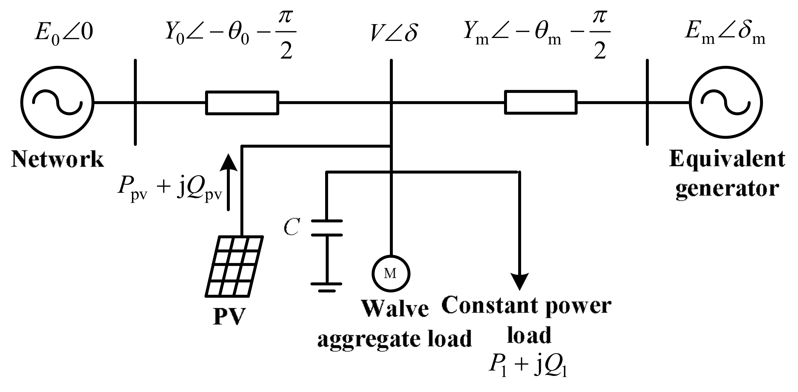
As shown in Figure 2, a large-scale PV power plant is integrated into a classic three-node system [5]. The three-node system is a classic model for studying voltage stability problems [28,29] and any complex system can be reduced to the form of a three-node system via equivalent transformation. Considering that most of the loads in power grids are induction motors, the load in Figure 2 is made up of the induction motor (Walve aggregate load model [28,29]) and the constant power load in parallel. As shown in Figure 2, C represents the shunt capacitor banks. The purpose of installing capacitor banks is to ensure that the load bus voltage amplitude is in a qualified range when the three-node system is running.

The ordinary differential equations (ODEs) of the system in Figure 2 are [9] given below:

$$\{\begin{array}{c}{\dot{\delta }}_{\mathrm{m}}=\omega \hfill \\ \dot{\omega }=\frac{1}{M}[-D\omega +P_{\mathrm{m}}+E_{\mathrm{m}}^2{Y}_{\mathrm{m}}\sin {\theta }_{\mathrm{m}}+E_{\mathrm{m}}V{Y}_{\mathrm{m}}\sin (\delta -{\delta }_{\mathrm{m}}-{\theta }_{\mathrm{m}})]\hfill \\ \dot{\delta }=\frac{1}{k_{q\omega }}(-k_{qV}V-k_{qV2}{V}^2+Q-Q_0-Q_1+Q_{\mathrm{pv}})\hfill \\ \begin{array}{cc}\hfill \dot{V}& =\frac{1}{T{k}_{q\omega }{k}_{pV}}[k_{p\omega }{k}_{qV2}{V}^2+(k_{p\omega }{k}_{qV}-k_{q\omega }{k}_{pV})V+\hfill \\ & k_{p\omega }(Q_0+Q_1-Q_{\mathrm{pv}}-Q)-k_{q\omega }(P_0+P_1-P_{\mathrm{pv}}-P)]\hfill \end{array}\hfill \end{array}$$

(3)

The active power P and the reactive power Q of the load demand from the network and equivalent generator are given below:

$$\{\begin{array}{c}P=-E{\prime }_{0}VY{\prime }_0\sin (\delta +\theta {\prime }_0)-E_{\mathrm{m}}V{Y}_{\mathrm{m}}\sin (\delta -{\delta }_{\mathrm{m}}+{\theta }_{\mathrm{m}})+(Y{\prime }_0\sin \theta {\prime }_0+Y_{\mathrm{m}}\sin {\theta }_{\mathrm{m}})V^2\\ Q=E{\prime }_{0}VY{\prime }_0\cos (\delta +\theta {\text{'}}_0)+E_{\mathrm{m}}V{Y}_{\mathrm{m}}\cos (\delta -{\delta }_{\mathrm{m}}+{\theta }_{\mathrm{m}})-(Y{\prime }_0\cos \theta {\prime }_0+Y_{\mathrm{m}}\cos {\theta }_{\mathrm{m}})V^2\end{array}$$

(4)

where the state variables δ_m and ω are, respectively, the rotor angle and angular frequency of the equivalent generator. The state variables δ and V are the voltage phase angle and the voltage amplitude of the load bus, respectively. P_pv and Q_pv are the active and reactive powers of the PV, respectively. P₁ and Q₁ are the active and reactive powers of the constant power load, respectively; P₀ and Q₀ are the constant active and reactive powers of the Walve motor load. See Appendix A for the meaning and values of the other parameters.

The equilibrium equations of the ODEs (3) are given below:

$$\{\begin{array}{l}\omega =0\hfill \\ -D\omega +P_{\mathrm{m}}+E_{\mathrm{m}}^2{Y}_{\mathrm{m}}\sin {\theta }_{\mathrm{m}}+E_{\mathrm{m}}V{Y}_{\mathrm{m}}\sin (\delta -{\delta }_{\mathrm{m}}-{\theta }_{\mathrm{m}})=0\hfill \\ -k_{qV}V-k_{qV2}{V}^2+Q-Q_0-Q_1+Q_{\mathrm{pv}}=0\hfill \\ k_{p\omega }{k}_{qV2}{V}^2+(k_{p\omega }{k}_{qV}-k_{q\omega }{k}_{pV})V+k_{p\omega }(Q_0+Q_1-Q_{\mathrm{pv}}-Q)-k_{q\omega }(P_0+P_1-P_{\mathrm{pv}}-P)=0\hfill \end{array}$$

(5)

We took the reactive power Q₁ of the constant power load as the bifurcation parameter. The PV active power is set from P_pvmin to P_pvmax. From Equation (5), we can derive the system’s SNB point position difference between P_pvmax and P_pvmin (the detailed derivation process is given in Appendix B):

$$Q_{1\mathrm{SNBmax}}-Q_{1\mathrm{SNBmin}}=-a(V_{\mathrm{SNBmax}}^2-V_{\mathrm{SNBmin}}^2)+\tan {\varphi }_{\mathrm{pv}}(P_{\mathrm{pvmax}}-P_{\mathrm{pvmin}})$$

(6)

where Q_1SNB and V_SNB are the reactive powers of the constant power load and the load bus voltage, respectively, at the SNB point. The subscripts “max” and “min” represent the corresponding values when the PV active power is at P_pvmax and P_pvmin. They are the same in the following equation. $a=-k_{qV2}-Y{\prime }_0\cos \theta {\prime }_0-Y_{\mathrm{m}}\cos {\theta }_{\mathrm{m}}$. ϕ_pv is the power factor angle of the PV output power.

From the second equation of Equation (5), we obtained the following:

$$V_{\mathrm{SNB}}\sin ({\delta }_{\mathrm{SNB}}-{\delta }_{\mathrm{mSNB}}-{\theta }_{\mathrm{m}})=\frac{P_{\mathrm{m}}+E_{\mathrm{m}}^2{Y}_{\mathrm{m}}\sin {\theta }_{\mathrm{m}}}{-E_{\mathrm{m}}{Y}_{\mathrm{m}}}$$

(7)

where the calculation result of the right formula is fixed. δ_SNB and δ_mSNB represent the corresponding values at the SNB point.

By putting Equation (7) into Equation (6), the SNB point position difference between P_pvmax and P_pvmin can be calculated. If the plan and design of the power grid are reasonable, the voltage phase angle difference between both ends of the line is very small. When the fluctuation range of P_pv is not too large, the variable quantity of the (δ_SNB − δ_mSNB) value at the SNB point should be very small, and the variable quantity of the sin(δ_SNB − δ_mSNB − θ_m) value is smaller. It can be derived from Equation (7) that the value of (V²_SNBmax − V²_SNBmin) is also very small.

The range of the tanϕ_pv is generally from −0.2 to + 0.2 [9]. It can be seen from Equation (6) that the SNB point position difference between P_pvmax and P_pvmin is relatively large when tanϕ_pv ≠ 0. When tanϕ_pv = 0, the PV power plant runs in a unity power factor (cosϕ_pv = 1) and the SNB point position difference will decrease significantly.

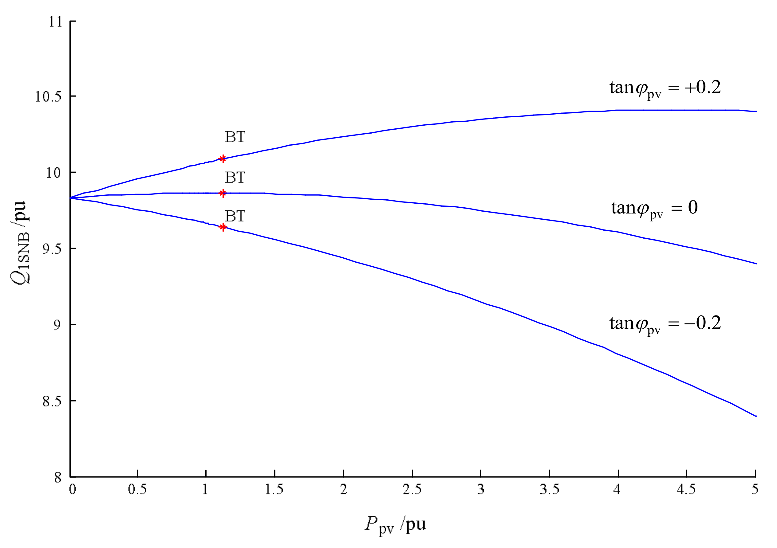
Next, we used the numerical bifurcation analysis software MATCONT to verify the above conclusions. We let P₁ = 0 pu and the load center capacitor banks C = 10 pu. Next, we took P_pv and Q₁ as the bifurcation parameters for the double-parameter bifurcation analysis. Figure 3 shows the P_pv-Q_1SNB curves calculated by the ODEs (3) when P_pv changes from 0 pu to 5 pu. We do not discuss where the BT (Bogdanov–Takens) bifurcation is a co-dimension bifurcation. It can be seen from Figure 3 that when tanϕ_pv = 0 and when P_pv < 2 pu, the change in Q_1SNB is minimal, and that when tanϕ_pv = ±0.2, Q_1SNB undergoes a relatively larger change. From the perspective of reducing the impact of the PV output fluctuation on the system’s voltage stability, the PV inverter should operate in a unity power factor, if possible.

The same conclusion can be obtained when the active power P₁ of the constant power load is taken as the bifurcation parameter.

From the above analysis we can see that when cosϕ_pv is 1 or close to 1 and when P_pv is not too large (generally no more than 1–2 pu), the impact of the PV output fluctuation on the SNB point position is minimal. It can be seen from Equations (1) and (2) that, for the same load power, the change in the load margin index value is smaller as well. Since any complex system can be equivalent to the three-node system shown in Figure 2, the above conclusion has a certain degree of universality.

Therefore, we can calculate the load margin index via the load power value at the SNB point when P_pv is P_pvmin, not considering the PV output fluctuation. Equations (1) and (2) can be expressed as the following:

$$I_{\mathrm{LM}}=1-\frac{P_0}{P_{\mathrm{SNBmin}}}$$

(8)

$$I_{\mathrm{LM}}=1-\frac{Q_0}{Q_{\mathrm{SNBmin}}}$$

(9)

where P_SNBmin and Q_SNBmin are the load’s active and reactive powers, respectively, at the SNB point when P_pv is P_pvmin.

P_SNBmin or Q_SNBmin can be calculated via the continuous power flow (CPF) method when P_pv is P_pvmin (usually at 0 pu). Since the impact of the PV output fluctuation is no longer considered, the calculation process of the load margin index I_LM can be greatly simplified and the calculation speed can evidently be improved. This is propitious to the on-line application of the load margin index.

4. The Design of Fuzzy Load-Shedding Strategy

We take the three-node system shown in Figure 2 as an example. The installed capacity of PV is 1 pu, and the PV runs in a unity power factor. We let P₁ = 0 pu and Q₁ be the bifurcation parameter. The MATCONT software (Version 2.4., Ghent University, Ghent, Belgium and Utrecht University, Utrecht, The Netherlands) is used for the analysis.

Table 1. The values of the load’s reactive power and the voltage at the saddle-node bifurcation (SNB) points of the three-node system with the photovoltaic cell (PV).

Ppv/pu	Q1SNB/pu	VSNB/pu
0	9.8310	0.8123
0.1	9.8371	0.8123
0.2	9.8425	0.8129
0.3	9.8473	0.8133
0.4	9.8515	0.8137
0.5	9.8550	0.8141
0.6	9.8580	0.8145
0.7	9.8604	0.8149
0.8	9.8621	0.8154
0.9	9.8633	0.8159
1.0	9.8638	0.8164

shows the load’s reactive power Q_1SNB and the voltage amplitude V_SNB of the system’s SNB point when the PV active power P_pv changes. It can be seen that Q_1SNB gradually increases with the increase of P_pv, but that the amount of change is minimal.

We then observe the changes of the load bus voltage. As can be seen from Table 1, no matter how the P_pv fluctuates, the voltage amplitude of the SNB point is higher (>0.81 pu), which results from the large capacity shunt capacitor banks (C = 10 pu) installed in the load center, thus, raising the voltage amplitude of the load bus. When the system runs close to the SNB point, the load margin becomes very small and more load should be shed to maintain the system’s voltage stability. However, when the voltage amplitude of the load bus is relatively high, the load may be shed less or not shed, causing a great risk to the safe and stable operation of the system. Besides the voltage amplitude of the load bus, we can introduce the load margin index as the basis for emergency load shedding so that the system can avoid this hidden danger.

Considering that the fuzzy control theory is applied to solve the uncertainty and deal with multi-target problems [30], a dual-input single-output fuzzy load-shedding controller is designed for the system shown in Figure 2. The voltage amplitude of the load bus and load margin index are used for the fuzzy input variables and a load-shedding command is used for the fuzzy output variable.

4.1. Principles of Load Shedding

The load margin index I_LM is calculated at the SNB point when P_pv = 0 pu. We set I_LM ≥ n₁~n₂ (0 < n₁ < n₂ < 1) when the system is running normally. For example, if a system requires a load margin of 15% to 20%, then n₁ = 0.15 and n₂ = 0.2. As shown in Figure 4, the principle of load shedding according to the load margin index can be specified. When I_LM < n₁, the voltage stability of the system is in a dangerous state and the load should be shed more. When n₁ ≤ I_LM < n₂, the voltage stability of the system is in an alert state and the load should be shed less. When I_LM ≥ n₂, the voltage stability of the system is in a stable state and the load does not need to be shed.

On the other hand, the acceptable range of the load bus voltage amplitude is generally above 0.9 pu when the power system operates normally. In this case, the principle of load shedding, according to the voltage amplitude of the load bus can be stated as follows: when V < 0.85 pu, the load should be shed more; when 0.85 pu ≤ V < 0.9 pu, the load should be shed less; when V ≥ 0.9 pu, the load does not need to be shed.

4.2. Fuzzy Variables, Fuzzy Domains, and Membership Functions

The fuzzy input variables of the designed dual-input single-output fuzzy load-shedding controller are the load margin index (ILM) and the load bus voltage amplitude V, while the fuzzy output variable is the load-shedding command (LS).

The fuzzy word set of ILM can be taken as {NB, NS, Z} according to the previously determined principle of load shedding, which indicates that the load margin index value is very small, smaller, and normal, respectively.

The fuzzy word set of V is taken as {NB, NS, Z}, which indicates that the voltage amplitude is very low, lower, and normal, respectively.

The fuzzy word set of LS is taken as {NLS, LLS, MLS}, which means no load shedding, less load shedding, and more load shedding, respectively. Setting the command to less load shedding and more load shedding can ensure the rationality of the load-shedding quantity and lead to avoiding losing an excessive load in the system. The load-shedding quantity can be set according to the specific operating conditions of the system.

Figure 5 shows the membership functions of the fuzzy input and output variables, where:

The fuzzy domain of the fuzzy input variable ILM is taken as the interval [0 1] and the membership function of the fuzzy subset NB, NS, and Z takes the trapezoidal, triangular, and trapezoidal functions, respectively. The parameters of the membership functions are the abscissa values corresponding to the vertices of the triangle or trapezoidal functions, and they are set according to the load margin index reference values of the load shedding. The parameters of the NS trapezoidal function are [0 0 n₁ (n₁ + n₂)/2]; the parameters of the NS triangular function are [n₁ (n₁ + n₂)/2 n₂]; and the parameters of the Z trapezoidal function are [(n₁ + n₂)/2 n₂ 1 1].

The fuzzy domain of the fuzzy input variable V is [0.8 1.2] and the membership functions of the fuzzy subset NB, NS, and Z take the trapezoidal function (the parameters are [0.8 0.8 0.85 0.875]), the triangular function (the parameters are [0.85 0.875 0.9]), and the trapezoidal function (the parameters are [0.875 0.9 1.2 1.2]), respectively. The parameters of the membership functions are set according to the load bus voltage reference values of the load shedding.

The fuzzy domain of the fuzzy output variable LS is [0 1]. The membership functions of the fuzzy subset NLS, LLS, and MLS take the Gaussian function (the parameters are [0.1699 0], [0.1699 0.5] and, and [0.1699 1], respectively).

4.3. Fuzzy Rules

Nine IF-THEN fuzzy rules of the fuzzy controller are extracted based on the above principles of load shedding, according to the load margin index and voltage amplitude of load bus, as shown in

Table 2. IF-THEN fuzzy rules.

	ILM	NB	NS	Z
V
NB		MLS	MLS	MLS
NS		MLS	LLS	LLS
Z		MLS	LLS	NLS

. The extraction principle of the fuzzy rules is that, if one of the input variables ILM or V is not in the qualified range, the fuzzy controller will output the load-shedding command. A different load-shedding command (more load shedding or less load shedding) will then be decided according to the reduction degree of the input variable.

The meanings of the nine IF-THEN fuzzy rules are:

(1)

IF ILM is NB and V is NB, THEN LS is MLS

(2)

IF ILM is NB and V is NS, THEN LS is MLS

(3)

IF ILM is NB and V is Z, THEN LS is MLS

In the above three rules, ILM is very small. In order to ensure that the power grid is able to recover to a state of normal operation, the fuzzy controller has to output the more load shedding command (MLS), no matter what state V is in.

(4)

IF ILM is NS and V is NB, THEN LS is MLS

(5)

IF ILM is Z and V is NB, THEN LS is MLS

In the above two rules, V is very small, so the fuzzy controller has to output the MLS to recover the bus voltage amplitude.

(6)

IF ILM is NS and V is NS, THEN LS is LLS

(7)

IF ILM is NS and V is Z, THEN LS is LLS

(8)

IF ILM is Z and V is NS, THEN LS is LLS

In the above three rules, either ILM is smaller or V is smaller and the other input variable is normal or smaller. Therefore, the fuzzy controller just needs to output the less load shedding command (LLS).

(9)

IF ILM is Z and V is Z, THEN LS is NLS

When ILM and V are all in the qualified range, the fuzzy controller does not operate (output is the no load shedding command (NLS)).

4.4. Fuzzy Reasoning and Anti-Fuzzification

The Mamdani reasoning is used in the fuzzy controller; when the fuzzy relation of each fuzzy rule is set to R_i (i = 1~9), then the fuzzy relation of the fuzzy control system is as follows:

$$R={\displaystyle \underset{i=1}{\overset{9}{\cup }}{R}_i}$$

(10)

where $\cup$ represents the union operation.

The output variable LS′ will then be calculated through the given input variables ILM′ and V′ according to the fuzzy supposing reasoning.

$$LS\prime ={[ILM{\prime }^{\mathrm{L}}\circ V\prime ]}^{\mathrm{H}}\circ R$$

(11)

where the superscript ‘L’ indicates the fuzzy column vector and the superscript ‘H’ indicates the fuzzy row vector. ‘$\circ$’ is the synthetic operator and the max-min synthesis is taken generally.

Figure 6 is the fuzzy surface of the designed fuzzy load-shedding controller. We can see that the smaller the quantization value of ILM or V, the greater the quantization value of LS is and the more inclined it is to load shedding.

The center-of-gravity method can be used in the anti-fuzzification of the output variable LS [30]. When the output quantization value is LS ≤ 0.3, the output variable can be specified as no load shedding, 0.3 < LS < 0.7 as less load shedding, and LS ≥ 0.7 as more load shedding.

4.5. Flowchart of Fuzzy Load Shedding

The process of fuzzy load shedding is shown in Figure 7. In this flowchart, after 5–10 s, the real-time operating data will be collected again and whether the two load-shedding commands are the same will be determined. The aim is to prevent the rapid change and recovery of the load power or PV output from causing the malfunction of the fuzzy controller.

5. Discussion on the Load-Shedding Quantity

The load-shedding quantity in the load-shedding control has always been a difficult problem. If the quantity is too small, it will be hard to maintain the system’s voltage stability and recover the voltage amplitude. If the quantity is too large, it will cause unnecessary load loss.

A practical load-shedding method is introduced to the fuzzy load-shedding controller designed in this paper. When setting the load-shedding quantity as ∆P or ∆Q, the increment of the load margin index achieved by Equations (8) or (9) after the load shedding is $\frac{\Delta P}{P_{\mathrm{SNBmin}}}$ or $\frac{\Delta Q}{Q_{\mathrm{SNBmin}}}$, respectively. It can be seen from Figure 4 that more load should be shed when the load margin index is I_LM < n₁. To ensure that I_LM recovers to n₂~1, the increment of the load margin index should meet the following conditions:

$$\frac{\Delta P}{P_{\mathrm{SNBmin}}}\ge n_2-n_1$$

(12)

Or

$$\frac{\Delta Q}{Q_{\mathrm{SNBmin}}}\ge n_2-n_1$$

(13)

Therefore, the minimum load-shedding quantity for more load shedding is as follows:

$$\Delta P_{\mathrm{Min}.\mathrm{mls}}=(n_2-n_1)P_{\mathrm{SNBmin}}$$

(14)

Or

$$\Delta Q_{\mathrm{Min}.\mathrm{mls}}=(n_2-n_1)Q_{\mathrm{SNBmin}}$$

(15)

On the other hand, in order to avoid load over shedding, we can take 1 − n₂/(n₂ − n₁) times the minimum load-shedding quantity in the actual operation.

Similarly, for the case of less load shedding, we can derive that the maximum load-shedding quantity is as follows:

$$\Delta P_{\mathrm{Max}.\mathrm{lls}}=(n_2-n_1)P_{\mathrm{SNBmin}}$$

(16)

Or

$$\Delta Q_{\mathrm{Max}.\mathrm{lls}}=(n_2-n_1)Q_{\mathrm{SNBmin}}$$

(17)

In the actual operation, we can take 0.5–1 times the maximum load-shedding quantity.

Regardless of the situation, whether it is more or less load shedding, if the output LS of the fuzzy load-shedding controller is large, the load-shedding quantity will take a larger multiple, and if the output LS is small, the load-shedding quantity will take a smaller multiple.

6. Simulation Analysis for the Fuzzy Load-Shedding Strategy

6.1. Fuzzy Load Shedding in a Classic Three-Node System with a Large-Scale PV

Taking the system shown in Figure 1 as an example (the installation capacity of the PV power plant is 1 pu), we analyze the load-shedding effect of the designed fuzzy controller. We set the load margin index I_LM ≥ 0.1–0.15 when the system runs normally. The membership function parameters of the three fuzzy subsets NB, NS, and Z of the fuzzy input variable ILM are: [0 0 0.1 0.125], [0.1 0.125 0.15], and [0.125 0.15 1 1], respectively. The fuzzy inference system (FIS) file of the fuzzy controller is established using the MATLAB Fuzzy toolbox (Version R2010b. The MathWorks, Inc., Natick, MA, USA).

Scenario 1: The PV active power output P_pv = 1 pu, the parameters at the current operating point are as follows: (δ_m ω δ V Q₁) = (0.3462 0 0.1437 0.9817 9.3899), Q_1SNBmin = 9.8310 pu (can be seen from Table 1). According to Equation (9), I_LM = 1 − 9.3899/9.8310 = 0.045, which is much smaller than 0.1–0.15, so the system is in heavy load and close to the edge of voltage collapse. The quantization values of the fuzzy input variables ILM and V are substituted into the fuzzy controller and the quantization value of the fuzzy output variable is LS = 0.868 > 0.7, so the fuzzy controller outputs the MLS.

Now, although the voltage amplitude (0.9817 pu) is qualified, the value of I_LM is very small, so more load needs to be shed. At this moment, the load will not be shed according to the traditional UVLS strategy and the voltage collapse will occur in the system once the load creates a fluctuation. According to Equation (15), the minimum load-shedding quantity ∆Q_1Min.mls = (0.15 − 0.1) × 9.8310 = 0.49 pu and the range of the load-shedding quantity is (1–3) ∆Q_1Min.mls. As LS is relatively larger, the load-shedding quantity takes 1.47 pu (3 × 0.49). After the load shedding and the system recovers stability, V = 1.153 pu, and I_LM = 1 − 7.9199/9.8310 = 0.194. When putting the two values into the fuzzy controller again, we get LS = 0.132 < 0.3, so the load does not need to be shed.

Following this, if the weather suddenly becomes extremely terrible and the P_pv suddenly drops to 0 pu, after the system is stable, V = 1.145 pu, I_LM = 0.194 pu, and LS = 0.132 < 0.3; the fuzzy controller will output the NLS and the load will not need to be shed.

Scenario 2: The PV active power output P_pv = 0.5 pu, the parameters at the current operating point (δ_m ω δ V as Q₁) = (0.2949 0 0.1040 1.0909 8.5276), the calculated I_LM = 1 − 8.5276/9.8310 = 0.133, so the LS = 0.449 (between 0.3 and 0.7) and a small amount of load quantity needs to be shed. According to Equation (17), the maximum load-shedding quantity ∆Q_1Max.lls = (0.15 − 0.1) × 9.8310 = 0.49 pu. As LS is relatively smaller, the load-shedding quantity is set to 0.245 pu (0.5 × 0.49 = 0.245). After the load shedding and the system is stable, V = 1.115 pu and I_LM = 1 − 8.2826/9.8310 = 0.158, so we get LS = 0.132 < 0.3, and the load does not need to be shed again.

From the above analyses, we can see that the designed fuzzy controller has a better control effect on the load-shedding in the classic three-node system with a large-scale PV and it contributes to avoiding the voltage instability threat of SNB.

6.2. Fuzzy Load-Shedding in an IEEE 14-Bus System with a Large-Scale PV

The IEEE 14-bus system with a large-scale PV power plant is used to further verify the control effect of the designed fuzzy load-shedding controller. As shown in Figure 8, a large PV power plant (installation capacity is 1 pu) is integrated into Bus 5 with a unity power factor. The power supplies installed in Bus 3, Bus 6, and Bus 8 are all synchronous compensators (SCs), and all synchronous generators and SCs have automatic voltage regulators (AVRs) installed within them. The initial total load power of the system is 2.59 + j0.814 pu.

We assume that the transformers of the system are all normal transformers with constant tap ratios. We take the total load’s active power P as the bifurcation parameter. The SNB points of the system under the different PV active power outputs are obtained via a CPF method. The CPF method adopts the mode of the whole loads growing at the same time. The load’s active power values P_SNB of the SNB points when the PV active power output P_pv changes are shown in

Table 3. The values of the load’s active power at the SNB points of IEEE 14-bus system with PV.

Ppv/pu	PSNB/pu
0	6.1557
0.1	6.1922
0.2	6.2248
0.3	6.2517
0.4	6.2763
0.5	6.2958
0.6	6.3116
0.7	6.3232
0.8	6.3305
0.9	6.3336
1.0	6.3380

. It can be seen that the random fluctuation of the PV active power output has little effect on the SNB position. Therefore, when P_pv = 0 pu, the P_SNBmin (6.1557 pu) can be used to calculate the load margin index I_LM according to Equation (8).

Each load bus in the system includes the installation of the fuzzy load controller and takes local control of the load on the bus. The design of the fuzzy load-shedding controller installed in each bus is basically the same as that described in Section 4, except that the parameter settings of the fuzzy subset membership functions of the fuzzy input variable ILM are different. Supposing that it is required that I_LM ≥ 0.15–0.2 when the system is running normally, the membership function parameters of the three fuzzy subsets NB, NS, and Z of the ILM are [0 0 0.15 0.175], [0.15 0.175 0.2], and [0.175 0.2 1 1], respectively.

Now we give an example to describe the local control effect of the fuzzy load shedding. When P_pv = 0.5 pu and the system’s total load power is (2.59 + j0.814) × 2 = 5.18 + j1.628 pu, then the system is in heavy load. Take Bus 14 as an example. At this time, V = 0.9584 pu and I_LM = 1 − 5.18/6.1557 = 0.159. When putting the two values into the fuzzy controller, LS = 0.635, between 0.3 and 0.7, so a LLS needs to be carried out.

We calculated that the fuzzy load-shedding controllers installed in other buses all output the LLS, as shown in

Table 4. The fuzzy outputs of all the fuzzy load-shedding controllers of the IEEE 14-bus system with PV.

Bus	V/pu	ILM	LS	Load-Shedding Command
2	1.0450	0.159	0.635	LLS
3	1.0100	0.159	0.635	LLS
4	0.9772	0.159	0.635	LLS
5	0.9863	0.159	0.635	LLS
6	1.0700	0.159	0.635	LLS
9	0.9805	0.159	0.635	LLS
10	0.9804	0.159	0.635	LLS
11	1.0171	0.159	0.635	LLS
12	1.0347	0.159	0.635	LLS
13	1.0200	0.159	0.635	LLS
14	0.9584	0.159	0.635	LLS

. At this point, all the bus voltage amplitudes are qualified due to the voltage support of the SCs, but the load margin index I_LM is smaller, so the less load shedding needs to be carried out. According to Equation (16), the maximum load shedding quantity ∆P_Max.lls = (0.2 − 0.15) × 6.1557 = 0.31 pu, and the range of the load-shedding quantity is (0.5–1)∆P_Max.lls. As LS is close to 0.7, the load-shedding quantity takes 0.31 pu (1 × 0.31 = 0.31). We assume that the percentage of the load-shedding quantity of each bus is 6% (0.31/5.18 = 6%) when the system recovers stability after the load shedding, following which the parameters of Bus 14 are as follows: V = 0.9627 pu and I_LM = 1 − 4.87/6.1557 = 0.209 > 0.2. When putting the two values into the fuzzy controller, we get LS = 0.132 < 0.3 and the load doesn’t need to be shed again. The control effects installed in other buses are also the same.

In the IEEE 14-bus system, T2 sometimes adopts a load tap changing transformer (LTC) which is used for voltage stability research [16]. The LTC regulates the bus voltage or reactive power by changing the tap under the load. Now, when assuming that T2 is a LTC with a secondary voltage control mode and that the secondary reference voltage is 1.0129 pu, the tap ratio step is 0.005 and the dead zone is at 5%.

We set P_pv = 0 pu. The system’s total load power is at the initial value, the tap ratio of the LTC is at 1.090 pu by power flow calculation. From this operation point, we can calculate that P_SNB = 6.1036 pu using the CPF method (strictly speaking, this is an approximate value). When P_pv changes, the corresponding values of P_SNB are shown in

Table 5. The values of the load’s active power at the SNB points of the IEEE 14-bus system with PVs including a load tap changing transformer (LTC) regulation.

Ppv/pu	LTC Tap Ratio/pu	PSNB/pu
0	1.090	6.0136
0.1	1.095	6.1375
0.2	1.095	6.1676
0.3	1.095	6.1937
0.4	1.100	6.2142
0.5	1.100	6.2336
0.6	1.100	6.2494
0.7	1.100	6.2631
0.8	1.100	6.2751
0.9	1.100	6.2797
1.0	1.100	6.2800

. It can be seen that the impact of the LTC regulation on the value of P_SNB is minimal when the system is in a steady-state operation, and the system load margin has a slight decrease compared with Table 3. The P_SNBmin (6.0136 pu) can be used to calculate the index I_LM.

Now we set P_pv = 0.5 pu. Assume that the system’s total load power is 5.18 + j1.628 pu. At this time, I_LM = 1 − 5.18/6.1036 = 0.151. It can be seen from

Table 6. The fuzzy outputs of all the fuzzy load-shedding controllers of IEEE 14-bus system with PV including an LTC regulation.

Bus	V/pu	ILM	LS	Load-Shedding Command
2	1.0450	0.151	0.818	MLS
3	1.0100	0.151	0.818	MLS
4	0.9662	0.151	0.818	MLS
5	0.9801	0.151	0.818	MLS
6	1.0700	0.151	0.818	MLS
9	1.0129	0.151	0.818	MLS
10	1.0075	0.151	0.818	MLS
11	1.0311	0.151	0.818	MLS
12	1.0372	0.151	0.818	MLS
13	1.0251	0.151	0.818	MLS
14	0.9798	0.151	0.818	MLS

that although most load bus voltage amplitudes (the italic digits) are raised by LTC, I_LM is very small (close to 0.15) and all the fuzzy load-shedding controllers output the MLS at this time. According to Equation (14), the minimum load-shedding quantity is ∆P_Min.mls = (0.2 − 0.15) × 6.1036 = 0.31 pu and the range of the load-shedding quantity is (1–4)∆P_Min.mls. As LS is relatively larger, the load-shedding quantity takes 0.62 pu (2 × 0.31 = 0.62). After the load-shedding commands are carried out and the system is stable, I_LM = 1 − 4.56/6.1036 = 0.253 > 0.2 and all bus voltage amplitudes and the load margin index will return to normality; all the fuzzy controllers output the NLS.

From the above analyses, we can see that the designed fuzzy load-shedding controller also has a better control effect in the multi-machine power system with a large-scale PV plant. Even though the regulation function of the LTC is considered, the fuzzy load-shedding strategy can still play an important role in improving the static voltage stability of PV grid-connected systems.

7. Conclusions

In this paper, the impact of the PV output fluctuation on the position of the SNB point is derived based on the equilibrium point equations of a classic three-node system with a large-scale PV power plant, firstly. We found that when the PV plant is running with a power factor of 1 or close to 1 and the installed capacity of the PV plant is not too large (usually not more than 100–200 MW), the PV output fluctuation had little effect on the SNB position of the system and the impact on the load margin index was smaller. Consequently, the voltage stability load margin index can be calculated by the SNB point when the PV plant active power P_pv is at a minimum (usually at 0 pu). This greatly simplifies the calculation process of the load margin index and shortens its calculation time, creating the conditions for the on-line utilization of the load margin index in a large-scale PV grid-connected system. Since any complex system can be reduced to the form of a classic 3-node system by equivalent transformation, the conclusion has a certain degree of versatility.

On the other hand, large capacity reactive power compensation devices at the load center (for example, the shunt capacitor banks in classic three-node systems and the SCs in IEEE 14-bus system) will significantly increase the voltage amplitude of a load bus. It is, therefore, difficult to detect whether a power grid runs on the edge of a voltage collapse, which can cause a great threat to the safe and stable operation of the power grid. Meanwhile, the traditional UVLS strategy cannot maintain static voltage stability. Based on the above analyses, we proposed a fuzzy load-shedding strategy for SNB, while the impact of the PV output fluctuation was also taken into account. The input variables of the fuzzy load-shedding controller were the voltage amplitude of the load bus and the load margin index, and the output variable was the load-shedding command. The load margin index was calculated at the SNB point when P_pv is 0 pu and the selection principle of the membership function parameters of each input/output variable was determined. Nine fuzzy load-shedding rules were extracted and a practical calculation method for the load shedding that is quantity suitable for the fuzzy controller was also discussed. The fuzzy controller was simple in design and had a strong portability for different PV grid-connected systems.

The fuzzy load-shedding strategy overcomes the defect of the traditional UVLS method and the simulation analysis results for a classic three-node system and an IEEE 14-bus system with a large-scale PV verified the effectiveness of the designed fuzzy strategy. It can maintain the static voltage stability of the power grid and it can ensure that the voltage amplitude of the load bus is qualified.

The fuzzy load-shedding strategy designed in this paper is suitable for power grids integrated with PV power plants whose scale is at a level of several hundred MW and below and it can also be used as an emergency control measure to ensure the safe and stable operation of PV grid-connected systems.