Experimental and Numerical Simulation of the Heat Transfer Enhancement on the Twin Impingement Jet Mechanism

Abstract

This article presents a study which sought to enhance heat transfer by employing a twin jet impingement mechanism (TJIM) and investigating the impact of the distance between the nozzles and plate on the Nusselt number (Nu) and heat transfer coefficient. This investigation was additionally based on the measurements of the heat flux temperature micro foil sensor and IR thermal imaging. A computational study of the cooling heated plate, through simulating the electronic components by the TJIM, was investigated using the RNG k-ε turbulence model. The jet-plate position was changed at the different jet-to-plate distances S = 1, 6, and 11 cm, Reynolds number = 17,000. The main flow structure, the static pressure, local and average Nus and heat transfer coefficient, were also examined. The findings have yielded new information about TJIM, and represent a new contribution about the flow and heat transfer characteristics of TJIM, and means of improving the rate of heat transfer in the passive heat transfer technique. The results of the various positions of the TJIM determined that the first model is, in fact, the best model for the heat transfer coefficient and the highest Nu, when S = 1 cm and H = 1 cm. Furthermore, the irregular distribution of the local Nu and the local heat transfer coefficient (h) on the impinged surface are due to the increase or decrease in the turbulence of flow on the measured surface.

1. Introduction

Impingement jets are widely used in many engineering applications, especially in last few decades, to enhance heat transfer rates [1,2,3]. In this study, experimental and numerical methods are employed to investigate twin impingement jet flow and impingement heat transfer. The results from the experimental work and simulations are then analysed and discussed, along with the impacts relating to the heat transfer that occurred due to the impingement of the twin jets on the hot plate surface. The study further investigates the twin impingement jet flow, by examining the influence and effects of applying different parameters, such as Nozzle-Nozzle spacing and Nozzle-plate distance [4,5]. The flow characteristics of twin jets incorporate the velocity of the air jet in the external hole when the Reynolds number is equivalent to 17,000. The issues associated with heat transfer are correlated using five factors that affect heat transfer, and where further investigation of the heat transfer enhancement associated with the twin jets impingement is conducted. Importantly, the experiments in this study were performed following a complete verification of the experimental setup [6].

In this article, a computational study is undertaken on the cooling of industrial and engineering components, in an attempt to enhance the heat transfer coefficient [7]. Jet impingement has a significant impact on the cooling process of a flat surface, as well as on electronic applications [8,9]. Many researchers over the years have been motivated by the characteristics associated with heat transfer in the cooling process [9,10]. The flow and heat transfer characteristics of a single jet impingement mechanism on the protrusion surface have been investigated using numerical simulation and particle image velocimetry (PIV) [11]. A ground fast cooling simulation device was employed to investigate the impact of arrangement and nozzle geometry on the impinging jet’s heat transfer [12]. Large eddy simulation was carried out to study the flow dynamics and heat transfer characteristic of multiple impinging jets at high Reynolds numbers, and in a hexagonal configuration [13]. A numerical investigation and design optimization were carried out for impingement cooling system with an array of air jets [14].

However, there has been limited research to investigate the twin impingement jets mechanism numerically and experimentally. Accordingly, one of the key objectives of the present study is to simulate the characteristics of heat transfer in twin jets on a heated plate surface which is cooled by TJIM at different jet positions. This provides information on the most suitable model through the best heat transfer rate from different arrangements of jets on the surface measured, and is of considerable significance in the performance of industrial applications, and in efforts to improve the rate of heat transfer in passive heat transfer techniques using TJIM. The current study is conducted both experimentally and numerically, based on ANSYS FLUENT software (version 18, Ansys, Inc., Canonsburg, PA, USA). SOLIDWORKS software (Dassault Systèmes SolidWorks Corporation, Waltham, MA, USA) will be used to create and grid the system geometry, and to simulate the cases for the geometry model with two jets.

Turbulence Model

Computational Fluid Dynamics (CFD) provides a qualitative (and sometimes even quantitative) prediction of fluid flows for solving problems, which consists of four subject domains: geometry and grid generation, establishing a physical model, solving it, and post-processing the computer data. Using this approach, many of the CFD problems may be solved along with the acquired data that is computed using several tools to assist in creating the correct geometrical designs and grid patterns. However, no single model suits all conditions or requirements—especially for industrial and engineering applications—for establishing a physical model for turbulence flows, given that all models differ in some way. The importance of understanding the influencing factors for selecting the right model is paramount and often requires researching previous models used by other researchers that touch upon heat transfer and turbulence models, including their limitations and advantages.

Therefore, in selecting an appropriate turbulence model, many factors may influence the final decision, including: the physics associated with the overall flow model, whether the model is based on a proven method and approach, resolving of specific problems, the level of accuracy, assumptions, resource requirements, and computing power required to process large volumes of data quickly and precisely. Often overlooked is the allocated time needed for the simulation exercise, as this can be considerable, and may require additional processing power and effort.

One model that has been commonly used by many researchers is referred to as the common K-epsilon (k-ε) model, due to its abilities to provide accurate results, its affordability, the fact that it is relatively straightforward to implement and provides reasonable predictions for many flows, and that it has been widely used to simulate mean flow characteristics for turbulent flow conditions [15]. Notably, this model has been used to investigate turbulent flow problems through various simulation exercises and experiments in many countries.

Furthermore, what makes the K-epsilon (k-ε) model stand out, is that it is a two-equation model which gives a general description of turbulence using two transport equations, partial differential equation (PDEs): turbulent kinetic energy (k) and turbulent dissipation rate (ε), which are solved, and the eddy viscosity (μ_t) is computed as a function of k and ε. The Boussinesq hypothesis is also part of this model, given its low computational cost, and is applied to model the Reynolds stress term.

Therefore, in applying this model, several assumptions are made. The working fluid is air, and the flow characteristics are: steady flow, Newtonian fluid, an incompressible fluid, and turbulent flow. The Boussinesq approach also utilizes the Boussinesq hypothesis to reduce the Reynolds stresses to the mean velocity gradients as given below in Equation (1):

$$-\rho \overline{{u^{\prime }}_i{u^{\prime }}_j}= {\mu }_t\left(\frac{\partial {\overline{U}}_i}{\partial x_j}+\frac{\partial U_j}{\partial x_i}\right)-\frac{2}{3}\left(\rho k+{\mu }_t\frac{\partial {\overline{U}}_i}{\partial x_i}\right){\delta }_{ij }$$

(1)

where the eddy viscosity (${\mu }_t$) at each grid point is related to the values of the ($k$) and ($\epsilon$), [16]:

$${\mu }_t=\rho C_{\mu }\frac{k^2}{\epsilon }$$

(2)

Moreover, where $C_{\mu }$ is an empirical constant; and $k$ is the turbulent energy is defined by the fluctuating velocities as:

$$k = \frac{1}{2}\frac{1}{(u^2+v^2+w^2)}$$

(3)

The assumption here is that the flow is entirely turbulent, and the impact of the molecular viscosity is negligible.

2. Experimental Procedures and Methodology

Two types of impingement plates form part of the experimental setup according to the application of jet impingement heat transfer. First, an electrically heated plate is used for the jet impingement cooling application, and second, the thin film relatively cold plate is used in the hot jet impingement application. Accordingly, in both plates, a heat flux was generated due to the temperature difference between the air jet and the plate surface. Furthermore, the impingement plate surface used for the cooling application was designed and fabricated to be used as a heat source [17]. 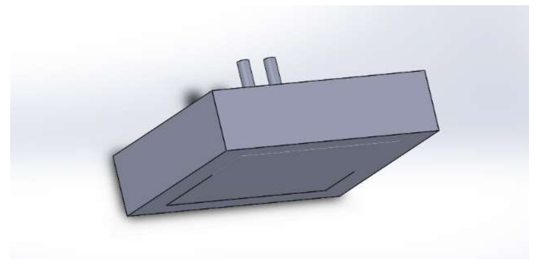The plate was made of aluminum, chosen for its high thermal conductivity (204 W/m·K) and light weight (2707 kg/m³) [18]. The dimensions of the plate were 4 mm × 300 mm × 300 mm; an electric plate heater of equivalent surface dimensions were fixed onto the back of the plate, and a steel plate supported the back of the heater with the same surface dimensions. All three components were then bolted together and fixed to an aluminum frame holder. It was possible to adjust the height of the plate. The impingement plate of the cooling application is shown in Figure 1.

The experimental procedures consisted of five steps:

• For each jet in the steady state, the airflow was initially set to acquire a Reynolds number of 17,000 by measuring the twin jet middle (center) point velocity at the nozzle exit using a pitot tube.
• To measure the flow rate and steady jet flow, a flow meter anemometer was installed in a constant temperature mode of 100 °C by Dantec Dynamics, who specialize in the development, manufacture and application support of measurement systems. Next, the flow meter was positioned between the refrigerated air dryer and the TJIM pipes, which pass through to the twin jets. It is important in this step to verify the speed of the flowmeter from the pitot tube through to the operation of the twin impingement jets. By capturing the heat transfer per unit (q) via the data logger, the highest Reynolds number is determined by calculating the convective heat transfer coefficient (h) by the units (W/(m²·K)). From the measured surface, the average Nu is then obtained for the points at the radial distance on the surface from the stagnation point.
• In this step, differential pressure produces a pressure difference as an analog that is then inputted to the data acquisition Ni 6008 device, which converts it to a signal. Using the Scilab code (developed beforehand), the signal is converted to a value. Notably, the differential pressure occurs between the pitot tube and the Ni 6008 data acquisition device.
• Three models are next constructed for the experimental tests using aluminum foil at a measured distance of 1, 6 and 11 cm from the nozzle exit and surface, with spacing between the nozzles of 1 cm. The purpose of this step is to allow measurements of the heat flux and surface temperature to be taken on the impingement surface.
• To capture the thermal images and temperature distribution at the surface, an infrared thermal imager (Fluke Ti25) is used to simultaneously capture images at the surface region until heat transfer to the steady state is achieved. When the heat inlet to the aluminum foil by the jets equals the heat loss by the effect of natural convection, heat transfer is achieved. During this step, to minimize errors in the heat flux temperature, several samples were recorded, to determine the average values. (see Figure 2 and Figure 3).

Before conducting the tests, various constant parameters were maintained related to the infrared thermal imager and TJIM as shown in

Table 1. Constant values in the numerical and experimental tests.

Constant Parameters	Values
Nozzle to Plate distance	1, 6 and 11 cm
Nozzle to Nozzle spacing	1 cm
Reynolds Number	17,000
Nozzle Diameter	0.02 m
Ambient Temperature	24 °C
Aluminum plate Temperature	100 °C
Emissivity of foil Aluminum	0.97
Transmission	100%

.

Next, the fluid mechanics and heat-transfer are considered in addressing the problems of jet impingement heat transfer, and consequently, the dimensionless numbers that are related must also be specified. The computation of the Reynolds number (the velocity) of the twin air jet—which correlates to the inertial forces because of viscous effects—is given as follows [19]:

$$Re=\frac{\rho \nu d}{\mu }$$

(4)

where μ represents the fluid’s dynamic viscosity (Pa·s or kg/(s) or N·s/m²), ν signifies the fluid velocity x (m/s), and ρ denotes the fluid density (kg/m³).

Forced convection dominated during the jet impingement heat transfer. The Newton’s law equation can be employed to determine the heat-transfer coefficient (h), i.e., [20] Q = h(T_s − T_j), which then gives:

$$h=\frac{q}{T_s-T_j}$$

(5)

where T_s represents the surface temperature, T_j signifies the air jet temperature and q denotes the amount of heat flux (W/m²).

The Nu equation is used to calculate the ratio of convective to conductive heat transfer, as follows [19]:

$$Nu=\frac{hd}{k}$$

(6)

where h indicates the convective heat-transfer coefficient, d represents the pipe diameter, and k signifies the fluid’s thermal conductivity.

3. Theoretical and Numerical Solution

3.1. Governing Equations

A series of governing equations are established as follows:

• The governing equations to be solved include the momentum, continuity and energy equations [21,22].
• The mass of fluid is conserved.
• According to (Newton’s second law), the rate of change in momentum is equal to the sum of the forces on a fluid particle.

According to the first law of thermodynamics, the rate of change of energy is equal to the sum of the rate of heat added, and the rate of work performed on a fluid particle.

$$\frac{\partial u}{\partial x}+\frac{\partial u}{\partial y}+\frac{\partial w}{\partial z}=0$$

(7)

$$\begin{array}{c}u\frac{\partial u}{\partial x}+u\frac{\partial u}{\partial y}+w\frac{\partial u}{\partial z}=-\frac{1}{r}\frac{\partial p}{\partial x}+n\left[\frac{{\partial }^{2}u}{\partial x^2}+\frac{{\partial }^{2}u}{\partial y^2}+\frac{{\partial }^{2}u}{\partial z^2}\right]\\ u\frac{\partial u}{\partial x}+u\frac{\partial u}{\partial y}+w\frac{\partial u}{\partial z}=-\frac{1}{r}\frac{\partial p}{\partial y}+n\left[\frac{{\partial }^{2}u}{\partial x^2}+\frac{{\partial }^{2}u}{\partial y^2}+\frac{{\partial }^{2}u}{\partial z^2}\right]\\ u\frac{\partial w}{\partial x}+u\frac{\partial w}{\partial y}+w\frac{\partial w}{\partial z}=-\frac{1}{r}\frac{\partial p}{\partial z}+n\left[\frac{{\partial }^{2}w}{\partial x^2}+\frac{{\partial }^{2}w}{\partial y^2}+\frac{{\partial }^{2}w}{\partial z^2}\right]\end{array}$$

(8)

$$u\frac{\partial T}{\partial x}+u\frac{\partial T}{\partial y}+w\frac{\partial T}{\partial z}=\frac{k}{r{c}_p}+n\left[\frac{{\partial }^{2}T}{\partial x^2}+\frac{{\partial }^{2}T}{\partial y^2}+\frac{{\partial }^{2}T}{\partial z^2}\right]$$

(9)

3.2. Description of the Numerical Model and Mathematical Formulation

3.2.1. Geometrical and Flow Description

The schematic diagram of a twin jet impingement mechanism (TJIM) of the three models that depend on the spacing between the nozzle and distance between the nozzle and plate and the cross-flow between the twinjet and the impinging plate is illustrated in Figure 4. The dimensions of the identical twin jets diameter are 0.02 m; the impingement plate width (W), height (H), and thickness (Z) are 0.3, 0.3 and 0.04 m respectively; the velocity of the jet flow equals Re is 17,000.

3.2.2. FLUENT Software Package

The flow equations are solved using two modules:

• The first module is a pre-processor module, a program structure that creates the geometry and grid using ANSYS FLUENT for:

  (a)

  Modeling of the geometry;

  (b)

  Mesh generation; and

  (c)

  Boundary condition.

• The second module is the ‘Solution’ module, for solving the Navier-Stokes equations (which include momentum, continuity and energy equations), as well as the turbulent flow model.

3.3. Mesh Generation

There are two kinds of approaches used in volume meshing: structured and unstructured meshing. FLUENT can use grids comprising of tetrahedron or hexahedron cells in three dimensions. However, the type of mesh selection depends on the application.

In a structured mesh, the governing equations are transformed into the curvilinear coordinate system aligned with the flat surface. While it is trivial for simple shapes [23], it becomes incredibly inactive and time consuming for complex geometries, and therefore is excluded in this study. In the unstructured process, the integral form of the governing equations is discretized, and either a finite-volume or a finite-element scheme is used. The information regarding the grid is directly inserted into the discretization. Unstructured grids are generally successful for complex geometries, rather than applications such as that described above. Notably, unstructured tetrahedron grids were used in the present work. A higher order element type is used for mesh generation to approximate the precise the boundaries of high curvature, including the following:

• For a three-dimensional mesh, a higher order tetrahedral element with hanging nodes (i.e., nodes on faces that are not vertices of all the cells sharing those faces) is used.

3.3.1. Three Dimension Mesh Generation

Although many mesh generation codes (e.g., FLUENT and ANSYS) support mesh generation of solid geometry and three-dimensional models from a single phase with minimum input from the user, it is more durable to divide this process into subsequent steps, including the following two key issues to further control the mesh [24].

3.3.2. Surface Mesh Generation

The surface mesh is created for the flat aluminum surface, the TJIM, and other boundaries as follows:

(a)

The edges are meshed by assigning an interval size for each boundary comprising a closed loop of the area;

(b)

The meshed edges are controlled by specifying a grading scheme for each edge;

(c)

On the edges of the mesh, a triangular element is used to generate a three-dimensional pave unstructured surface mesh.

3.3.3. Volume Mesh Generation

For the surfaces meshed for each region, the volume mesh can next be created for each area comprising of a closed loop of the area using the T-Grid, ANSYS scheme. Notably, building the mesh requires fine cells in the zones near the surfaces and edges in a TJIM. Furthermore, the mesh should be manipulated and controlled manually to maintain a smooth mesh transition, and to retain accurate mesh for a three-dimensional model. Moreover, with a minimal computational expense, this is accomplished by applying the size function. The features of the cases : the relevance center used was medium, the normal curvature angle of 12-degrees, the minimum size = 3 × 10⁻⁴, max face size 4 × 10⁻³, and the max Tet size 4 × 10⁻³ (see Figure 5).

3.3.4. Mesh Quality and Mesh Dependency

The generation of the mesh and mesh control for the three-dimensional model has been previously discussed in this article. Therefore, it is important to assess the mesh for both quality and dependency before running to guarantee that accurate results are successfully achieved. Furthermore, there are some general guidelines to produce good mesh, known as the rules of QRST standing for Quality, Resolution, Smoothness, and Total cell count [25].

3.3.5. Quality of Mesh

Investigating the mesh quality and to check the orientation of the elements is important. The face alignment represents the importance of the quality parameter; it is the parameter that calculates skewness of the cells. Also, the elements with high skewness should be averted. The face skewness can be calculated as given in Equation below as:

$$face skewness=1-\frac{leangth of shorter face diagonal }{leangth of longer face diagonal}$$

(10)

Accordingly, this value is about (0.2–0.5) according to [24].

3.3.6. Mesh Resolution

The grid-dependence analysis is held by creating a grid with more cells and to compare the solutions of the two models. The grid refinement tests for the average static temperature on a hot surface indicated that a grid size of approximately (one million cells) could produce sufficient accuracy and resolution to adopt as the standard for the models. Furthermore, the number of cells should be more near viscosity, influencing areas like the walls and the smaller at non-critical zones.

3.3.7. Total Cell Count

The last point in producing a good mesh is through the total number of cells produced. Accordingly, it is necessary to acquire a sufficient number of cells to achieve a good resolution, but memory requirements will increase as the number of cells increase. For the current case, an average of one million cells was used, and the number of iterations is the maximum number of iterations performed before the solver terminates, and in the present case, 3000 iterations were carried out.

3.4. Boundary Conditions

The boundary conditions are prescribed at all boundary surfaces of the computational domain. The mainstream conditions were maintained in all cases as follows:

• Plate temperature = 100 °C.
• Air velocity (Re) = 17,000.
• Dimension of plate = 0.3 × 0.3 × 0.04 m.
• Nozzle diameters = 0.02 m.

3.5. Results and Discussion

3.5.1. Model Validation

The cooling process adopted for engineering and industrial applications within the manufacturing industry has employed many models. One of the most popular models is the RANS turbulence model given the advantages associated with this approach for predicting the heat transfer procedure and the model’s minimal computational time. In the present chapter, the RNG k-ε turbulence model simulates all the cases of the twin impingement jets mechanism on the aluminum plate surface. Validation of the present model was undertaken using the experimental results of the average heat transfer coefficient presented by [6] for the same operating conditions and geometry. Indeed, the experimental results will determine the heat transfer coefficient numerically on the plate surface. Also, it was observed that the distribution of the average heat transfer coefficient had a minimal deviation from the experimental data and reported a good agreement with the experimental data, as illustrated in Figure 6.

The distribution of the average heat transfer coefficient (h) on the aluminum surface for all models at Reynolds number = 17,000 of the twin impingement jet mechanism is shown in Figure 6. The temperature distribution over a flat surface for the different models is illustrated in the above table to validate the simulation model. Also, it is observed that the distribution of the average heat transfer coefficient had a slight variation from the experimental data and reported a good agreement with the experimental data. The percentage of thermal enhancement factor resulting from the difference in the arrangement of the nozzles in the three models was approximately 10% to 20% as indicated in

Table 2. Error Percentage of heat transfer coefficient (h) between the Numerical and Experimental tests.

Model No.	Parameter	Numerical Tests (h)	Experimental Tests (h)	Percentage of Error
1	S = 1 & H = 1	51.76	56.55	8.47%
2	S = 1 & H = 6	44.55	50.19	9.43%
3	S = 1 & H = 11	41.59	46.02	9.62%

.

The concave profile on the front face is also in good agreement with the experimental data. The results show that the higher values of the heat transfer coefficient were obtained on the first model when S = 1 and H = 1.

3.5.2. Experimental Results on Twin Impingement Jet Mechanism

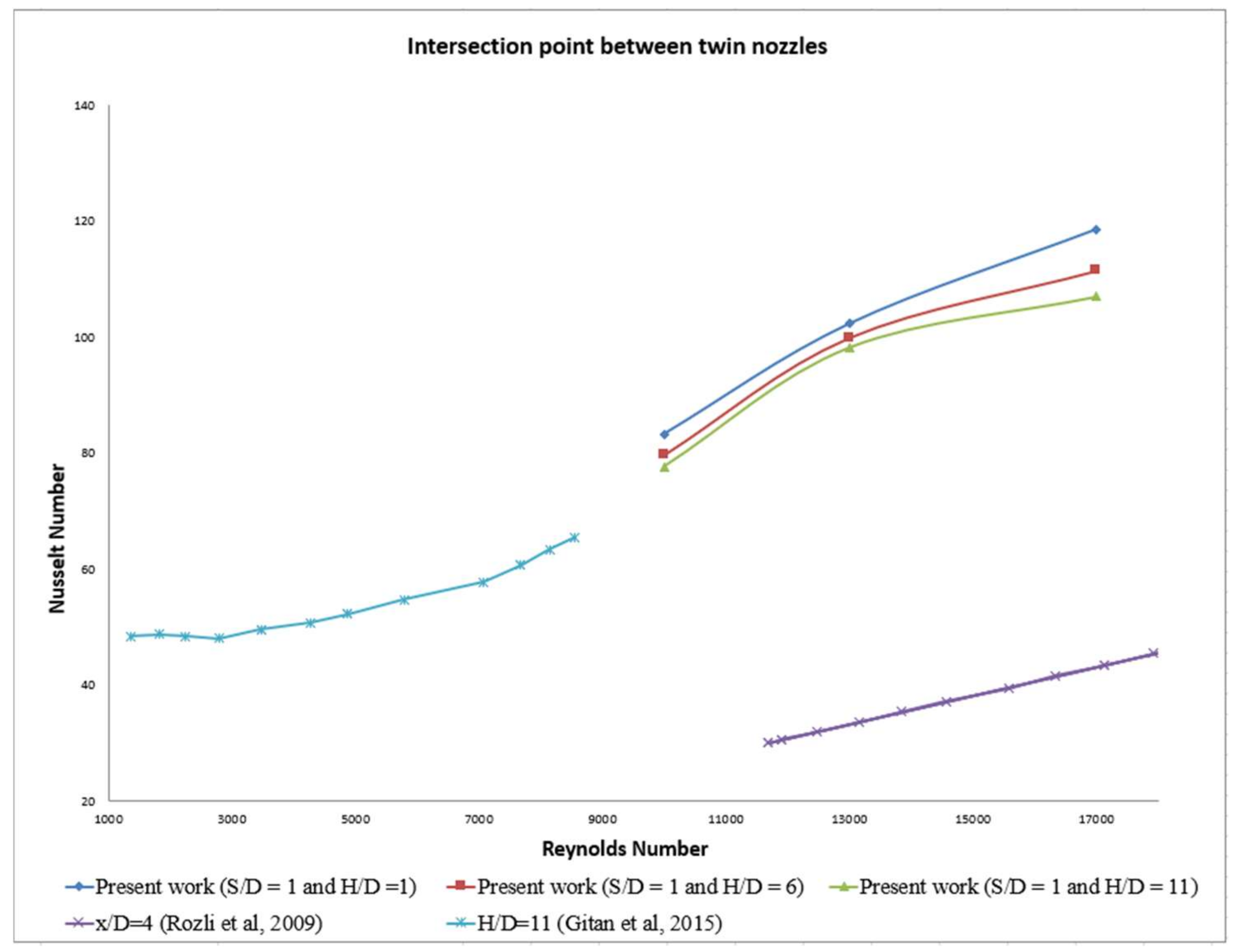
The experimental setup of TJIM was verified through performing several tests and through comparing the data obtained with other work. The analyses of the air leakage, flow characteristics, heat transfer performance, and the thermal behavior at the impingement surface were conducted to verify the overall setup and the twin jets performance. The work of [26] was selected for comparative purposes in this study, due to the similarities between their experimental setup and the present work. However, there are several differences between both practices that were considered in the comparison of the results. The “Test Results in The Interference Zone of Twin Jets Impingement” as shown in Figure 7, illustrates the intersection of the Nu and the Reynolds number at a nozzle-nozzle spacing equal to 1 cm, and the nozzle-plate distance equal to 1, 6 and 11 cm subsequently. Obviously, the Nu at the near nozzle-plate distance level is higher than that at the high nozzle-plate distance level. Furthermore, at all nozzle-plate spacing distances, the Nu increases as the Reynolds number increases with a similar slope. Indeed, this slope similarity denotes a similar effect on the Nu which is performed as the nozzle-plate distance varies at all considered Reynolds number levels. Also, there is a noticeable enhancement in Nu compared with the other results [27].

Figure 7 displays the intersection of the Nu at the nozzle-nozzle spacing equal to 1 cm, and the nozzle-plate distance equal to 1, 6 and 11 cm subsequently. Obviously, the Nu at the near nozzle-plate distance level is higher than that at the high nozzle-plate distance level. Moreover, at all nozzle-plate spacing distances, the Nu increases as the Reynolds number increases with a similar slope. Indeed, this slope similarity denotes the similar effect on the Nu which is performed as the nozzle-plate distance varies at all considered Reynolds number levels. There is a noticeable enhancement in the Nu comparing with another result.

3.5.3. Thermal Image

Figure 8 presents the images captured by a thermal imager and illustrate how the twin jets impingement mechanism (TJIM) is affected and distributed on the plate surface that measures the impinged target. The images are labeled with the center of the temperature values. The illustrated steady jet cases below are based on three models. The images were captured for all models, with one image captured for each model at Re = 17,000. Furthermore, in these images, some observations can be made. First, the hottest spots can be observed due to the impact of the twin jets impingement. Secondly, the midlevel point of temperature, an elliptical temperature distribution can be observed, and higher temperature rates were achieved through the steady jet case because of the high flow rates for the jets. In contrast, in TJIM, due to its duty principles, the lower flow rate was supplied. Figure 8 also displays the higher center temperature of 82.6 °C when H = 1 and S = 1 (i.e., the first model). Notwithstanding, the twin jets had the highest temperature result to the high sensitivity of the thermal imager that can detect even the smallest temperature changes between both jets.

3.6. Convective Heat Transfer

Numerical simulations are performed using the RNG k-ε model to investigate the cooling process on the flat plate heated by an electrical heater using the TJIM for the three models according to jet-jet spacing (S) = (1 cm), jet-plate distance (H) = (1, 6 and 11 cm) and the Reynolds number at 17,000. The impact of the jet position on the average Nus and heat transfer coefficient are examined. The values of the average Nu and heat transfer coefficient (h) are chosen based on the jet-jet spacing and jet-plate distance.

The distribution of the heat transfer coefficient (h) on the aluminum surface for all the models at the Reynolds number =17,000 of the twin impingement jet mechanism is shown in Figure 9. The temperature distribution over a flat surface for the different models are: (a) S = 1 and H = 1 (b) S = 1 and H = 6 (c) S = 1 and H = 11. It can be observed that the distribution of the average heat transfer coefficient has a convex profile on the front face that is in good agreement with the experimental data. The results show that the higher values of the heat transfer coefficient are obtained on the first model when S = 1 and H = 1. The remaining models, as seen from the images, are not dissimilar from each other regarding thermal distribution. The jet arrangement will help to determinate the turbulence intensity in the air flow that limits the distribution of the heat transfer coefficient and reflecting the impacts of the twin jets on the plate surface.

3.6.1. Model (1) Nozzle-Nozzle Spacing = 1 cm, and Nozzle-Plate Distance = 1 cm

For Model 1, when the spacing between the nozzles is equivalent to 1 cm, and the distance between the nozzle and plate equals 1 cm, the contour of the predicted static temperature for the k-ε model for model 1; displays contours of the total temperature, as presented in Figures below. A tiny part for the thermal distribution of the hot plate as shown in Figure 10 below, displays the heat transfer coefficient being high in the middle of the plate surface and then decreases gradually when moving away from the plate center. Furthermore, the high-temperature region is located on the plate surface where the presence of strong recirculating air flow exists resulting from the twin jet under high velocity. The remaining models, as shown in the figures below, are not dissimilar from each other. The surface Heat Transfer Coefficient in this model (h) = 51.76 (W/m²·K).

The distribution of the fluctuating heat transfer coefficient (h) is presented in Figure 11. Notably, these distributions display many characteristics which are like the mean heat transfer coefficient distributions. The peak in the magnitude of the fluctuations occurs at the stagnation points of the twin jets, which gradually decreases moving from the center of the stagnation points.

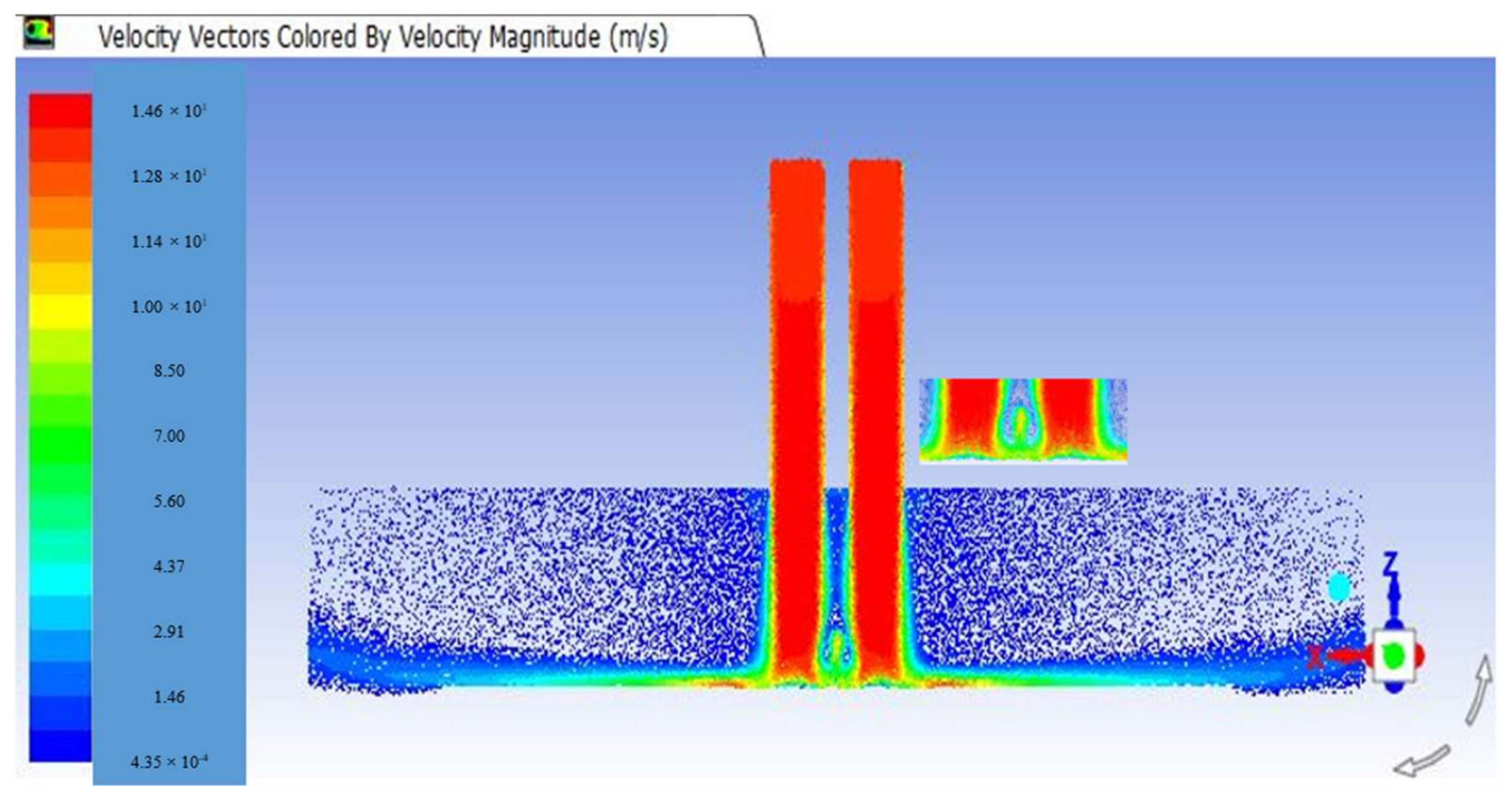
The velocity vectors and temperature contours in the below-mentioned models, (Figure 12 and Figure 13) illustrate the combined plot of the velocity vectors colored by the velocity magnitude and the temperature contours for all cases of the models described above. From these figures, it is evident that an air flow on the heated flat plate surface and the apparent turbulence on the aluminum plate occurs mainly when the jets become too close to the plate surface. Furthermore, it is also observed that the flow directions have changed and that swirls are generated, in-turn increasing the disturbance that leads to the increased heat transfer coefficient and thus increases the Nu. The temperature attained on the plate surface was 100 °C with the air velocity Reynolds number was equal to 17,000.

3.6.2. Model (2) Nozzle-Nozzle Spacing = 1 cm and the Nozzle-Plate Distance = 6 cm

Figure 14, Figure 15, Figure 16 and Figure 17 present the contours of the static temperature of the cooling process for the plate surface for Model 2 when the nozzle-nozzle spacing is equivalent to 1 cm, and the nozzle-plate distance equals 6 cm. The contour of the predicted static temperature for the k-ε model for model 1; the contours of the total temperature is presented in Figure 15. The high-temperature region is located on the plate surface where the presence of strong re-circulating air flow results from the twin jet under high velocity. The temperature is 100 °C, and the Surface Heat Transfer Coefficient in this model (h) = 44.55 (W/m²·K).

The shape of the heat transfer coefficient distributions shown in Figure 14 indicates that the heat transfer decreases dramatically when moving away from the direction of the stagnation point. Once again, the difference is more pronounced at different parameters such as an increase or reduction in the S and H values.

The velocity vectors and temperature contours in the below-mentioned model, (Figure 16 and Figure 17) show the combined plot of the velocity vectors which are colored by the velocity magnitude and the temperature contour for the second model. From these figures, it is evident that an air flow on the heated flat plate surface and the noticeable turbulence on the aluminum plate occurs mainly when the Jets are near to the plate surface. The flow directions are also observed to have changed, and swirls are generated, thereby increasing the disturbance leading to the increased heat transfer coefficient and in-turn, increases the Nu.

3.6.3. Model (3) Nozzle-Nozzle Spacing = 1 cm and the Nozzle-Plate Distance = 11 cm

For Model 3 when the spacing between the nozzles is equivalent to 1 cm, and the distance between the nozzle and plate is equal to 11 cm, the contour of the predicted static temperature for the k-ε model for model 2; contours of the total temperature are presented below. Also, a tiny part representing the thermal distribution of the hot plate is shown in the figures below, heat transfer coefficient is high in the middle of plate surface then decreases gradually when moving away from the plate center. The high-temperature region is located on the plate surface where there is the presence of a strong recirculating flow of air that is originating from the twin jet under high velocity. The Surface Heat Transfer Coefficient in this model = 41.59 (W/m²·K).

By observing the heat transfer coefficient distributions at different points with the vortex development, a better understanding of the influence of the vortices can be achieved. Figure 18 presents the heat transfer distributions at the low nozzle to the impingement surface spacings. The axial heat transfer coefficient distributions are consistent with the flow behavior and the heat transfer coefficient. Figure 19, Figure 20 and Figure 21 below present the contours of the static temperature of cooling process for the plate surface for model 3 when the nozzle-nozzle spacing is equivalent 1 cm and the nozzle-plate distance is equal to 11 cm. The contour of the predicted static temperature for the k-ε model for model 3; contours of the total temperature is also presented in the figures. The high-temperature region is located on the plate surface where the presence of strong re-circulating air flow air is observed coming from the twin jet under high velocity.

The values of the Nu exhibited a reasonable change with an increase or decrease in the distance values [28]. These results appear more logical when comparing to other research works [29]. Moreover, when the steady or where the impinging air twin jets on a hot plate surface occur near the interference zone’s center line passing through all the twin jets’ holes towards the end of the surface plate [30]. Accordingly, this section presents the results from the experimental data. Also, the figures above demonstrate the effect of TJIM on the surface temperature as measured through a heat flux-temperature sensor placed on the front of the flat plate surface and the thermal image on the surface. Indeed, at the first 4 or 5 points, there was an observed increase in the surface temperature on the plate surface, which then begins to gradually decrease after the 5-point measured distance on the aluminum surface plate [6].

It is important also to demonstrate how TJIM can impact the Nu in the midpoint or center between the air twin jets passing to the end of the interference zone near the terminal aluminum plate surface. The figures demonstrate how the Nu numbers are influenced based on the measurements by the micro-foil sensors. The recorded Nu number was found to decrease with increases in the distance from the center of the aluminum plate surface towards the terminal of the surface (low rates at distant points away from the flat plate surface center). Accordingly, this result was logical, as well as the simulation and experiment, where the increase in the heat-transfer rate occurred until the twin jets were near to the flat plate surface. Especially, when under the direct impact experienced by the heat flux sensor under the twin jets air flow on the surface. There was a gradual decrease in the distance from the center of the interference zone. However, this was an increase when compared to other research studies.

Eventually, as presented in the figures of the heat transfer coefficient distribution, this indicated that the heat transfer gradually decreases when moving away from the direction of the stagnation point. Likewise, the difference is more evident at different parameters such as an increase or reduction in the spacing between the nozzles and the distance between the nozzle and plate. Furthermore, there is an apparent mixing of air in the intersection area between the nozzles, as well as the presence of the measured area under the direct effect of the air coming from the nozzles, which decreases when the spacing increases between the nozzles and in-turn, increases the distance between the nozzle and plate.

3.7. Conclusions

Numerical simulation and experimental work were carried out based on the RNG k-ε turbulence model and TJIM to investigate the cooling process of a heated aluminum plate surface using TJIM in three different models. The impact of the jet position (i.e., the ‘Jet-Plate’ distance) and the high Reynolds number on the convective heat transfer to obtain the average heat transfer coefficient and average Nu. The main conclusions drawn from the study are that the temperature distribution over a flat surface for the different models is demonstrated to validate the simulation model. Secondly, it was also observed that the distribution of the average heat transfer coefficient had a slight variation from the experimental data and was reported to be in good agreement with the experimental data. Therefore, in summary, the findings have given more information about TJIM that has not been done before to provide the new contribution about the flow and heat transfer characteristics of TJIM. The main conclusions from work performed in this study are:

(a)

Simulation of three models at the Reynolds number = 17,000 was used to compare and validate the results comparing with the experimental tests.

(b)

The jet position was investigated (as the jet-plate distance), influencing the heat transfer coefficient, the average Nu and distribution of static pressure.

(c)

The contour of the predicted static temperature, the velocity vector colored by the static temperature and the velocity vectors’ colored velocity magnitude for the k-ε model were captured and discussed.

(d)

The various positions of the TJIM showed that the first model (Model 1) is the best model for the heat transfer coefficient and the highest Nu when the S/D = 1 cm and H/D = 1 cm.

(e)

The irregular distribution of the local heat transfer coefficient and the local Nu on the impinged surface occurred due to the increase or decrease in the turbulence of flow on the measured surface.

(f)

The different twin jet arrangements demonstrated that the least model for the heat transfer coefficient and the Nu is the third model when the S/D = 1 cm and H/D = 11 cm.

(g)

Numerical validation of the results is achieved by comparing with the experimental data for the TJIM.

(h)

The different twin jet arrangements showed that the least model of heat transfer coefficient and the Nu is the third model when the S/D = 1 cm and H/D = 11 cm.

(i)

As the twin nozzles are close to each other, the nearest distance between the nozzle and impinged surface plate shows significant variation especially at interference zone more than that as nozzle-nozzle spacing increases.