A New Discharge Pattern for the Characterization and Identification of Insulation Defects in GIS

Abstract

Identification of insulation defects in gas insulated metal-enclosed switchgear (GIS) is important for partial discharge (PD) evaluation. This article proposes a polar coordinate pattern approach to characterize the different kinds of defect types. These defect types include floating electrodes, a fixed protrusion on the enclosure, surface contamination on the spacer, metallic prominence on the high voltage electrode, a void in the insulator, and free metal particles on the enclosure. First, the physical models for the insulation defects in the established GIS model are designed. Second, the phase resolved pulse sequence (PRPS) data sets are obtained using ultra-high frequency (UHF) measurement. Then, the polar coordinate patterns are proposed to characterize the defects. Nine discharge parameters combined with the parameters based on quadrant statistical theory constitute the input feature vector to identify the PD types. The experimental results show that these new parameters could produce a clear, quantitative description of the characteristics of the defect types and could be used to distinguish between the different kinds of defect types.

1. Introduction

In high-voltage power systems, gas insulated metal-enclosed switchgear (GIS) is widely used. Electrical insulation is an important problem in all high voltage power equipment; therefore, insulation fault detection is necessary. If an insulation fault existing inside GIS is not detected, it may cause insulation faults in the GIS. According to the CIGRE 23.10 investigation report, insulation faults are the main cause of accidents in GIS. If any insulation fault exists inside GIS [1], the intensity of the electric field around the insulation fault increases locally. In this case, it will cause partial discharge (PD). The insulation between two conductors does not need to be completely bridged when PD takes place across a portion of the insulation between them [2]. PD can cause progressive deterioration and, in the worst cases, insulation breakdown. PD is harmful to the normal operation of power equipment, etc., including GIS. Therefore, PD detection is considered an effective way to avoid insulation failure in GIS [3,4,5]. For PD detection, identifying the PD type is important [6,7,8].

To detect PD, different schemes such as electrical, acoustical [9], and ultra-high frequency (UHF) detection methods [10,11] have been developed in previous years to measure partial discharge pulses. Many researchers have studied and developed the UHF method [11,12,13]. UHF sensors can detect the electromagnetic waves generated by PD with a frequency range from 300 MHz to 3 GHz [14,15]. UHF monitoring of PD data has become a recognized technique due to its sensitivity and comparative immunity to noise. The PD evoked by the floating electrodes, a fixed protrusion on the enclosure, surface contamination on the spacer, metallic prominence on the high voltage electrode, a void in the insulator, and free metal particles on the enclosure are common in GIS. This paper, through experiments in the GIS test cavity, applies the UHF method to monitor the PD of the six types of defects in GIS.

Identification of the insulation defects is an important aspect for PD detection [16,17,18]. The discharge characteristic parameters of the PD pattern plot, statistical operators [19], Weibull distribution parameters [20], fractal characteristic parameters [21], and PD characteristics based on chaos theory [22] have been proposed to identify different discharge sources. Distance classifiers, statistical classifiers, Artificial Neural Network (ANN)-base classifiers, fuzzy logic based classifiers [23], and the Kernel Statistical Uncorrelated Optimum Discriminant Vectors (KSUODV) algorithm have been applied to undertake GIS PD pattern recognition [24]. Additionally, the support vector machine (SVM) method has been used for PD identification where successful applications have demonstrated that SVMs can perform as well or better than classical pattern recognition approaches [25].

This paper proposes a new analysis and identification method for the PD types in a GIS. First, the physical models for the PD are designed in the established 220 kV GIS model. Second, the phase resolved pulse sequence (PRPS) data sets are obtained by ultra-high frequency (UHF) measurements. Then, polar coordinate patterns are proposed to characterize the insulation defects. The polar coordinate pattern is classified into two clusters using the K-means clustering algorithm. From the clustering results, the nine discharge parameters, the centroid, the phase range, the PD number, the phase median, the phase quartile and the amplitude quartile, in terms of each cluster, were calculated. The discharge parameters were processed to obtain the cosine similarity, A_ratio1, and A_ratio2. Combined with the parameters based on quadrant statistical theory, these parameters constituted the input feature vector to identify PD types.

This paper compares the performance of a SVM classifier with traditional parameters versus one with new parameters. Through the experimental results, six types of insulation defects are identified by the parameters extracted from the polar coordinate pattern.

2. Experiment Setup and Physical Models of the Insulation Defects

2.1. Test Sample and Measuring System

The 220 kV GIS sample is shown in Figure 1a. The 220 kV GIS sample comprised a high voltage conductor, a metal enclosure, and spacer insulators. The test cavity was considered to be coaxial cylindrical electrodes. The internal diameter and the external diameter were 106 mm and 320 mm, respectively. The test chamber was 2700 mm long. The basin-shaped insulator was made of epoxy resin and its relative dielectric constant was 4. The outer diameter and the thickness of the insulator were 520 mm and 40 mm, respectively. The test conditions were consistent with the actual working conditions. The SF₆ gas was set to 0.4 MPa. The mounting hole was designed for the installation of the UHF internal sensor. The hand hole was reserved for the physical model placement. The positions of the PD source and UHF sensor are shown in Figure 1b.

The UHF sensor’s sensitivity was obtained with a pulsed gigahertz transverse electromagnetic (GTEM) cell. The ratio of the sensor’s output (volts) to the applied electric field (volts per mm) gave the resultant sensor sensitivity in terms of millimeters. The frequency range of the electromagnetic wave excited by PD was mainly in the range of 0.3–1.5 GHz. Therefore, the frequency response of the UHF sensor was measured in the range of 0–2 GHz. The sensor had a mean effective height of $H_e=10.2\mathrm{mm}$ over the frequency range of 500 MHz to 1500 MHz, as shown in Figure 2.

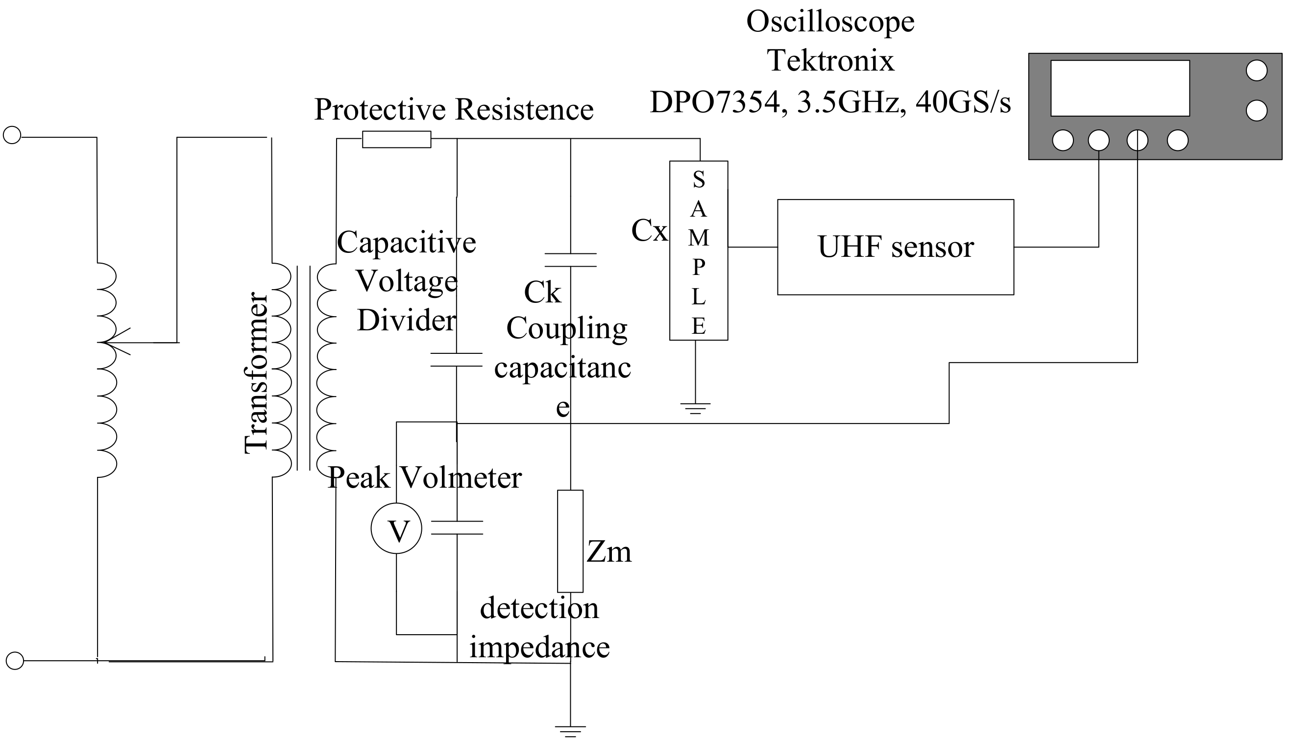
The measuring system is shown in Figure 3. The voltage regulator, transformer, and voltage divider comprised the measuring system. A corona-free discharge encapsulated transformer was used to produce the applied voltage. The rated voltage of the transformer was 750 kV, and the rated power was 375 kVA. The test voltage was adjustable within the range of 0–750 kV. $C_x$ presents the PD physical model in the GIS. $C_k$ is a 500 pF capacitor used for coupling the pulse current signals produced by $C_x$. $Z_m$ stands for the coupling impedance. The UHF PD signal was obtained by the internal UHF sensor. A Tektronix oscilloscope DPO7354 was used for data acquisition. The parameters for the oscilloscope were a 3.5 GHz bandwidth and a 40 GS/s max. sample rate.

2.2. Physical Models of the Insulation Defects

The physical models of the common insulation defects were designed as described below. The floating electrode defect in GIS, as shown in Figure 4a, was achieved by fixing a flat metal washer with a diameter of 33 mm to the High Voltage (HV) conductor. The HV conductor and the washer were separated from each other using insulation tape wrapped around the HV conductor. Figure 4b illustrates a metal protrusion on the enclosure. At the enclosure, a single metal protrusion with a length of 1.7 cm was fixed to simulate the corona discharge. A metal wire of 5.3 cm in length was located on the insulator to simulate the surface contamination on the spacer as shown in Figure 4c. One end of the wire was positioned close to the high conductor, but not contact in with it, with the other end pointing to the cylinder wall in the radial direction. Approximately 2.1 cm from the conductor, a metal protrusion was fixed to obtain the corona discharge on the conductor (Figure 4d). Figure 4e shows a void in the epoxy insulator. A hole was drilled into the insulator, and epoxy resin was used to seal the hole. A void formed after the coagulation. Figure 4f shows the free metal particles of 0.05–0.1 cm in width and 0.1–0.2 cm in length on the enclosure.

3. Proposal of the Polar Coordinate Pattern and Experimental Test

3.1. The New Proposed Discharge Pattern

The discharge region is discontinuous as a result of the positive and negative half cycle partition throughout the whole cycle when using the traditional phase resolved partial discharge (PRPD) pattern. As shown in Figure 5, when the applied voltage was 390 kV, the discharge region of the floating electrode defect was –30°~90°. This region was divided into –30°~0° (330°~360°) and 0°~90° in the PRPD pattern, but in practice, this region is continuous. The same situation for the surface contamination on the spacer defect was also detected.

If the discharge occurs at the positive and negative boundary of the power frequency voltage, using the floating electrode defect as an example, the phase ranges at the positive half cycle and the negative half cycle are 0°~90°, 150°~180° and 180°~270°, 330°~360°, respectively. As a result, the areas corresponding to 90°~150° and 270°~330° are blank. These blank areas divide the distribution of the discharge in the positive and negative half cycles into two parts. Due to the existence of this blank area, parameters such as the discharge width, phase center of gravity and discharge amplitude center of gravity extracted from the PRPD pattern cannot represent its original physical meaning. Statistical characteristic parameters, such as skewness, kurtosis, and asymmetry, based on the positive and negative half cycle partition also cannot represent the original statistical significance due to the existence of this blank region.

In order to solve this problem, this paper presents a method for drawing PD spectra in polar coordinates and obtaining the polar coordinate phase resolved partial discharge analysis pattern. In the polar coordinate pattern, the horizontal axis in the PRPD pattern is in a head to tail arrangement, so the observation of the partial discharge phase characteristics can be more intuitive. Additionally, the polar coordinate pattern is distinguished from its corresponding PRPD pattern by the fact that it applies a clustering algorithm. This approach does not use the traditional positive half cycle and negative half cycle analysis method. The new discharge parameters, in terms of each cluster extracted from the new polar coordinate pattern, can be used to better identify the defect type. The following section specifically describes the the steps of the polar coordinate pattern in detail.

3.2. Steps for the Polar Coordinate Pattern

The polar coordinate pattern proceeds according to the following steps.

Step 1

The PD data sets are prepared for the polar coordinate pattern. The data measured by the UHF method is stored as a sequence of PD pulses, $u_s(t_s,U(t_s))$, of which $t_s$ is the time of the PD pulse occurrence; $U(t_s)$ is the applied voltage; and $u_s$ is the discharge amplitude of the PD pulses. Data sets named the phase resolved pulse sequence (PRPS) data were selected for our tests. The PD data plotted in the polar coordinate takes the discharge amplitude, $u_s$, as the polar radius and the angle, $\phi$, as the polar angle.

Step 2

Normalize the discharge amplitude of PD pulses, $u_s$, using the Equation (1)

$$u_{\mathrm{norm}}=(u_s-u_{\min })/(u_{\max }-u_{\min })$$

(1)

where $u_{\min }$ is the minimum amplitude of the discharge, and $u_{\max }$ is the maximum amplitude of the discharge.

Step 3

Convert the degree value, $\phi$, from degrees to radians (${\phi }_{\mathrm{norm}}$).

Step 4

Use the 50 Hz applied voltage as the reference signal, and draw the PD data in the polar coordinate, using the discharge amplitude, $u_{\mathrm{norm}}$, as the polar radius and the angle, ${\phi }_{\mathrm{norm}}$, as the polar angle.

Step 5

Classify the partial discharge into two clusters using the K-means clustering algorithm. The K initial centroids are chosen, where K is a specified parameter. According to the measurement statistics and phase distribution characteristics of the partial discharge, K is specified as 2. The centroid of a cluster is the mean of the points in the cluster and is calculated as follows:

$$c_i=1/N_i{\displaystyle \sum _{x\in C_i}x}$$

(2)

where $C_i$ is the $i^{th}$ cluster; $x$ is a point in $C_i$, and $c_i$ is the mean of the $i^{th}$ cluster; $N_i$ is the PD number of each PD cluster.

Step 6

Calculate the discharge parameters where the centroids are indicated in the polar coordinate pattern. The 0.5th quartile (the median), the 0.25th quartile (the lower quartile), and the 0.75th quartile (the upper quartile) for the phase and discharge amplitudes are indicated in the polar coordinate pattern.

The polar coordinate pattern can be obtained through this approach. The polar coordinate patterns were 500 power cycles of the PRPS data sets.

3.3. Experimental Results

The experimental results of the six kinds of partial discharge proposed in the paper were 370 kV, 271 kV, 58 kV, 106 kV, 340 kV, and 540 kV, respectively. The voltage level was selected when the discharge was at a steady discharge state.

The six kinds of partial discharge were classified into two clusters by the K-means clustering algorithm. Then, the discharge parameters in terms of each cluster were calculated. The centroids marked in the polar coordinate patterns were calculated according to Equation (2) and are represented by $(c_{\phi },c_u)$ where $c_{\phi }$ is the phase angle of the centroid measured in degrees, and $c_u$ is the amplitude of the centroid; these are the mean of the points in the cluster. They describe the average level of each discharge region. The phase range was calculated according to the minimum and the maximum phase of the Cluster 1 PD and Cluster 2 PD. The PD numbers were calculated in terms of each PD cluster. The phase and the amplitude were analyzed through the quartile method. The 0.25 quartile (lower quartile), the 0.75 quartile (upper quartile), and the 0.5 quartile (the median) were calculated to measure the dispersion of the PD data sets and to analyze the characteristics of the partial discharge. The polar coordinate pattern for the six types of insulation defect are shown in Figure 6, Figure 7, Figure 8, Figure 9, Figure 10 and Figure 11. The discharge parameters calculated from the polar coordinate pattern are summarized in

Table 1. Parameters calculated from the polar coordinate pattern of the floating electrode defect.

Parameters	Centroid	Phase Range	PD Number	Phase Median	Phase Lower Quartile	Phase Upper Quartile	Amplitude Median	Amplitude Lower Quartile	Amplitude Upper Quartile
Cluster 1	(25°, 0.21)	[–18°, 93°]	334	24°	6°	39°	0.16	0.1	0.27
Cluster 2	(204°, 0.22)	[159°, 277°]	426	198°	189°	219°	0.19	0.1	0.32

,

Table 2. Parameters calculated from the polar coordinate pattern of the fixed protrusion on the enclosure defect.

Parameters	Centroid	Phase Range	PD Number	Phase Median	Phase Lower Quartile	Phase Upper Quartile	Amplitude Median	Amplitude Lower Quartile	Amplitude Upper Quartile
Cluster 1	(81°, 0.15)	[50°, 123°]	2444	80°	69°	93°	0.12	0.05	0.21
Cluster 2	(269°, 0.13)	[238°, 299°]	1002	270°	261°	278°	0.1	0.04	0.18

,

Table 3. Parameters calculated from the polar coordinate pattern of the surface contamination on the spacer defect.

Parameters	Centroid	Phase Range	PD Number	Phase Median	Phase Lower Quartile	Phase Upper Quartile	Amplitude Median	Amplitude Lower Quartile	Amplitude Upper Quartile
Cluster 1	(60°, 0.18)	[25°, 100°]	218	61°	53°	69°	0.11	0.06	0.22
Cluster 2	(223°, 0.10)	[197°, 285°]	161	216°	211°	227°	0.07	0.04	0.12

,

Table 4. Parameters calculated from the polar coordinate pattern of the metallic prominence on the high voltage electrode defect.

Parameters	Centroid	Phase Range	PD Number	Phase Median	Phase Lower Quartile	Phase Upper Quartile	Amplitude Median	Amplitude Lower Quartile	Amplitude Upper Quartile
Cluster 1	(82°, 0.16)	[43°, 120°]	1235	80°	69°	95°	0.13	0.09	0.22
Cluster 2	(260°, 0.15)	[215°, 300°]	1322	260°	244°	274°	0.15	0.08	0.20

,

Table 5. Parameters calculated from the polar coordinate pattern of a void in the insulator defect.

Parameters	Centroid	Phase Range	PD Number	Phase Median	Phase Lower Quartile	Phase Upper Quartile	Amplitude Median	Amplitude Lower Quartile	Amplitude Upper Quartile
Cluster 1	(72°, 0.18)	[36°, 109°]	67	67°	63°	78°	0.11	0.06	0.23
Cluster 2	(256°, 0.12)	[218°, 302°]	414	260°	241°	271°	0.09	0.04	0.17

and

Table 6. Parameters calculated from the polar coordinate pattern of the free metal particles on the enclosure defect.

Parameters	Centroid	Phase Range	PD Number	Phase Median	Phase Lower Quartile	Phase Upper Quartile	Amplitude Median	Amplitude Lower Quartile	Amplitude Upper Quartile
Cluster 1	(60°, 0.24)	[5°, 143°]	1239	59°	50°	71°	0.15	0.12	0.37
Cluster 2	(227°, 0.17)	[146°, 340°]	2800	232°	206°	247°	0.13	0.10	0.16

.

3.3.1. Floating Electrode Defect

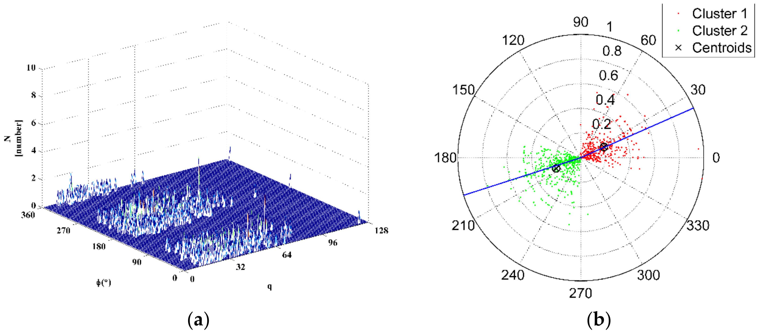
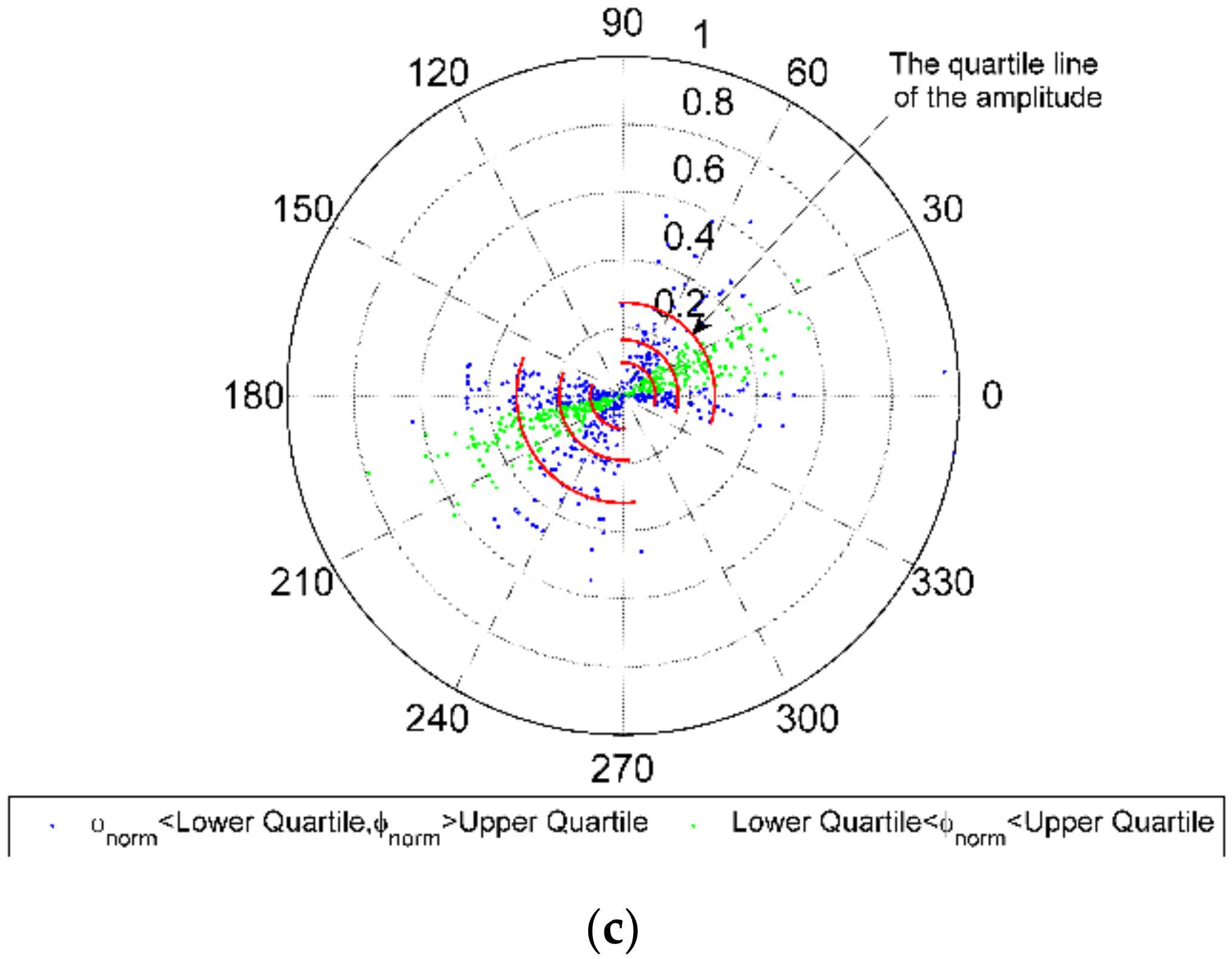
The PRPD pattern and the polar coordinate pattern for the floating electrode defect are shown in Figure 6. The discharge parameters calculated from the polar coordinate pattern are summarized in Table 1. The PRPD pattern is shown in Figure 6a. The cluster results are indicated in Figure 6b. The phase median lines were drawn in the polar coordinate pattern as shown in Figure 6b. The 0.25th quartile (lower quartile) and the 0.75th quartile (upper quartile) of the phase are indicated in Figure 6c. The blue color indicates areas that were in the range of ${\phi }_{\mathrm{norm}}$ < lower quartile and ${\phi }_{\mathrm{norm}}$ > upper quartile. The green color indicates the areas that were in the range of the lower quartile < ${\phi }_{\mathrm{norm}}$ < upper quartile.

With the PRPD pattern, the pulses were mainly concentrated in the phase intervals of 0°~90°, 150°~270° and 330°~360°. The discharge area was divided into three parts. In this type of phase distribution, the center phase at the negative half cycle may be less meaningful. The symmetry information cannot be observed from this pattern. However, more discharge information can be obtained from the polar coordinate pattern. The centroid of Cluster 1 was (25°, 0.21), and the centroid of Cluster 2 was (204°, 0.22). These were located in the first quadrant and the third quadrant. The phase median of Cluster 1 and Cluster 2 was 24°, 198°. The angle difference between the centroids was 179°. The phase median difference between Cluster 1 and Cluster 2 was 174°. This means that the centroids of the two clusters were almost in a straight line. The phase medians were also almost in a straight line. The centroid and phase medians of Cluster 1 and Cluster 2 were similar and symmetrical in the first and the third quadrants. The discharge of Cluster 1 was concentrated around the range of –18° to 93° and Cluster 2 was concentrated around the range of 159° to 277°. It was observed that the PD number of Cluster 1 was less than that of Cluster 2. The Cluster 1 discharge in the case where the lower quartile < ${\phi }_{\mathrm{norm}}$ < upper quartile was distributed mainly around the range of 6° to 39°, and the Cluster 2 discharge was centrally located in the range of 189° to 219°. These were mainly located in the first and third quadrants. It can be observed that the amplitude quartile value of Cluster 1 was similar to that of Cluster 2.

3.3.2. A Fixed Protrusion on the Enclosure Defect

The PRPD pattern and the polar coordinate pattern for the fixed protrusion on the enclosure defect are shown in Figure 7. The discharge parameters calculated from the polar coordinate pattern are summarized in Table 2. With the PRPD pattern, the discharge phase interval was concentrated within the ranges of 40°~120°, and 240°~300°. Compared to the polar coordinate pattern, PRPD could not exhibit the simplicity clearly. With the polar coordinate pattern, the centroid of Cluster 1 was (81°, 0.15), and the centroid of Cluster 2 was (269°, 0.13). The phase medians of Cluster 1 and Cluster 2 were 80° and 270°. It was observed that the PD number of Cluster 1 was more than doubled when compared with Cluster 2. As shown in Figure 7b, the phase median line almost went across the centroid in the cluster. The discharge of Cluster 1 was concentrated around the range of 50° to 123°, and the discharge of Cluster 2 was concentrated around the range of 238° to 299°. Cluster 1′s discharge in the case where the lower quartile < ${\phi }_{\mathrm{norm}}$ < upper quartile was concentrated around the range of 69° to 93° and Cluster 2′s discharge was concentrated around the range of 261° to 278°.

3.3.3. Surface Contamination on the Spacer Defect

The PRPD pattern and the polar coordinate pattern for surface contamination on the spacer defect are shown in Figure 8. The discharge parameters calculated from the polar coordinate pattern are summarized in Table 3. With the PRPD pattern, the phase interval was concentrated around the ranges of 0°~90° and 180°~270°. The difference between the positive and negative half cycles was not obvious. Nevertheless, the discharge parameters calculated from the polar coordinate pattern can provide more detailed information. The centroid of Cluster 1 was (60°, 0.18), and the centroid of Cluster 2 was (223°, 0.10). The phase median of Cluster 1 and Cluster 2 was 61°, 216°. The angle difference between the centroids was 163°. The phase median difference between Cluster 1 and Cluster 2 was 159°. This means that the centroids of Cluster 1 and Cluster 2 were not in a straight line. Similarly, the phase medians of the two clusters were not in a straight line. The discharge of Cluster 1 was concentrated around the range of 25° to 100°, and Cluster 2 was concentrated around the range of 197° to 285°. The density of Cluster 1 was less than that of Cluster 2. The Cluster 1 discharge in the case where the lower quartile < ${\phi }_{\mathrm{norm}}$ < upper quartile was concentrated around the range of 52° to 69°, and the Cluster 2 discharge was concentrated around the range of 211° to 227°. Figure 8c shows that the amplitude quartiles of Cluster 1 were higher than the amplitude quartiles of Cluster 2.

3.3.4. Metallic Prominence on the High Voltage Electrode Defect

The PRPD pattern and the polar coordinate pattern for the metallic prominence on the high voltage electrode defect are shown in Figure 9. The discharge parameters calculated from the polar coordinate pattern are summarized in Table 4. With the PRPD pattern, the discharge phase interval was concentrated within the ranges of 40°~120° and 210°~300°. With the polar coordinate pattern, the centroid of Cluster 1 was (82°, 0.16), and the centroid of Cluster 2 was (260°, 0.15). The phase median of Cluster 1 and Cluster 2 was 80°, 260°. It was observed that the PD number of Cluster 2 and the PD number of Cluster 1 was almost the same. As shown in Figure 9b, the phase median line almost went across the centroid in the cluster. The discharge of Cluster 1 was concentrated around the range of 43° to 120°, and Cluster 2 was concentrated around the range of 215° to 300°. The Cluster 1 discharge in the case where the lower quartile < ${\phi }_{\mathrm{norm}}$ < upper quartile was concentrated around the range of 69° to 95°, and the Cluster 2 discharge was concentrated around the range of 244° to 274°. The phase distribution characteristics obtained from the PRPD pattern and the polar coordinate pattern were similar to those for the fixed protrusion on the enclosure defect.

3.3.5. A Void in the Insulator

The PRPD pattern and the polar coordinate pattern for a void in the insulator defect are shown in Figure 10. The discharge parameters calculated from the polar coordinate pattern are summarized in Table 5. With the PRPD pattern, the discharge phase interval was concentrated within the range of 30°~100° and 210°~300°. With the polar coordinate pattern, the centroid of Cluster 1 was (72°, 0.18), and the centroid of Cluster 2 was (256°, 0.12). The phase median of Cluster 1 and Cluster 2 was 67°, 260°. It was observed that the PD number of Cluster 2 was more than the PD number of Cluster 1. The discharge of Cluster 1 was concentrated around the range of 36° to 109°, and Cluster 2 was concentrated around the range of 218° to 302°. The Cluster 1 discharge in the case where the lower quartile < ${\phi }_{\mathrm{norm}}$ < upper quartile was concentrated around the range of 63° to 78°, and the Cluster 2 discharge was concentrated around the range of 241° to 271°. The phase characteristics of the void in the insulator defect and the surface contamination on the spacer defect were similar.

3.3.6. Free Metal Particles on the Enclosure

The PRPD pattern and the polar coordinate pattern for the free metal particles on the enclosure defect are shown in Figure 11. The discharge parameters calculated from the polar coordinate pattern are summarized in Table 6. With the PRPD pattern, the discharge almost covered the whole phase range. The discharge was not concentrated in a specific area. With the polar coordinate pattern, the centroid of Cluster 1 was (60°, 0.24), and the centroid of Cluster 2 was (227°, 0.17). The phase median of Cluster 1 and Cluster 2 was 59°, 232°. The discharge of Cluster 1 was concentrated around the range of 5° to 143°, and Cluster 2 was concentrated around the range of 146° to 340°. The Cluster 1 discharge in the case where the lower quartile < ${\phi }_{\mathrm{norm}}$ < upper quartile was concentrated around the range of 50° to 71°, and the Cluster 2 discharge was concentrated around the range of 206° to 247°. The amplitude line almost formed a circle and showed that the phase region of the discharge involved almost every region.

4. Comparison between Recognition Accuracies

4.1. Traditional Feature Parameters Extraction

The statistical operators were introduced as the input feature vector to the classifier [19,26,27]. The selected statistical operators were calculated to describe the shape features of the PRPD patterns. The statistical operators contained skewness ($S_k$), kurtosis ($K_u$), the number of peaks ($P_e$), discharge asymmetry (Q), the cross-correlation factor (cc), and the modified correlation factor (mcc).

4.2. The New Proposed Parameters Extraction Method

The nine discharge parameters, including the centroid, phase range, PD number, phase median, phase quartile and amplitude quartile in terms of each cluster, as mentioned in Section 3, were processed to obtain the cosine similarity, $A_{ratio1}$, and $A_{ratio2}$. Combined with the parameters based on quadrant statistical theory, these parameters constituted the input feature vector to identify the PD types.

(1)

The parameter $D_i(i=1,2,3,4)$ is the percentage of discharge numbers at the first, second, third, and fourth quadrants accounting for the total PD number. $D_1$, $D_3$, $D_4$ are selected to form one of the part of feature vector.

(2)

The cosine similarity of centroids is calculated as

$$Cossim(c_1,c_2)=\frac{\langle c_1,c_2\rangle }{\Vert c_1\Vert \Vert c_2\Vert }$$

(3)

where $c_1$, $c_2$ are the centroids of Cluster 1 and Cluster 2, respectively.

(3)

This paper also used the ratio of the amplitude quartiles of Cluster 1 and Cluster 2. The formula is as follows.

$$A_{ratio1}=\frac{A{1}_{50}}{A{2}_{50}}or\frac{A{2}_{50}}{A{1}_{50}}(A_{ratio1}\ge 1)$$

(4)

$$A_{ratio2}=\frac{A{1}_{75}}{A{2}_{75}}or\frac{A{2}_{75}}{A{1}_{75}}(A_{ratio2}\ge 1)$$

(5)

where $A{1}_{50}$ is the 0.5 amplitude quartile (the median) of Cluster 1, and $A{2}_{50}$ is the 0.5 amplitude quartile (the median) of Cluster 2. $A{1}_{75}$ and $A{2}_{75}$ are the 0.75 amplitude quartiles of Cluster 1 and Cluster 2.

(4)

The skewness of Cluster 1 and Cluster 2 is defined as

$$\{\begin{array}{l}S{K}_x=\frac{1}{{\sigma }_x^3}{\displaystyle \sum _{i=1}^{N_1}{(x_i-\overline{x})}^3}\\ S{K}_y=\frac{1}{{\sigma }_y^3}{\displaystyle \sum _{i=1}^{N_1}{(y_i-\overline{y})}^3}\end{array}$$

(6)

$$\{\begin{array}{l}{x}_i=q_{\mathrm{norm}}{}_i\cos {\varphi }_{\mathrm{norm}}{}_i\\ y_i=q_{\mathrm{norm}}{}_i\sin {\varphi }_{\mathrm{norm}}{}_i\end{array}$$

(7)

where $x_i$, $y_i$ are the coordinates of each point in the polar coordinate pattern, calculated according to Equation (3). $\overline{x}$, $\overline{y}$ are the median values of the coordinates; and ${\sigma }_x$, ${\sigma }_y$ are the standard deviations of the coordinates. $N_1$ is the PD number of Cluster 1. The skewness of the Cluster 2 data sets is calculated in the same way.

(5)

The kurtosis of Cluster 1 and Cluster 2 is defined as

$$\{\begin{array}{l}K{U}_x=\frac{1}{{\sigma }_x^4}{\displaystyle \sum _{i=1}^{N_1}{(x_i-\overline{x})}^4-3}\\ K{U}_y=\frac{1}{{\sigma }_y^4}{\displaystyle \sum _{i=1}^{N_1}{(y_i-\overline{y})}^4-3}\end{array}$$

(8)

4.3. Experimental Procedures for PD Pattern Recognition

To verify the capability of the feature parameters extracted from the polar coordinate pattern to classify PD, this paper compared the performance of the support vector machine (SVM) classifier using the traditional feature parameters versus the new proposed parameters. SVM is known to be an effective method for dealing with prediction and classification problems [28]. In this paper, the SVM was used to undertake PD classification. For the SVM, a nonlinear transformation is needed to map the data from its original feature space into a new space where the decision boundary becomes linear. The method known as kernel trick is used to solve the curse of the dimensionality problem often associated with high-dimensional data. The choice in this work for the kernel function was the radial basis function (RBF) kernel.

$$K(x_i,x_j)=\exp (-\gamma {\Vert x_i-x_j\Vert }^2)$$

(9)

Table 7. Testing voltage level and number of samples of each defect model.

Label	Defect Model	Testing Voltage Levels (kV)	Number of Samples
1	Floating Electrode	296, 320, 350, 370, 390, 400	150
2	Fixed Protrusion on the Enclosure	210, 252, 271, 332, 370, 383	150
3	Surface Discharge	46, 53, 58, 61, 64, 69	150
4	Metallic Prominence on the High Voltage Electrode	73, 90, 106, 122, 140, 160	150
5	Void in an Insulator	247, 280, 320, 340, 360, 385	150
6	Free Metal Particles	502, 510, 520, 540, 560, 580	150

shows the testing voltage level and number of samples for each defect model. There were 150 samples for each defect model. The six kinds of defect models were labeled as 1, 2, 3, 4, 5, and 6 in the classification procedure. These 150 × 6 samples formed the experimental data sets.

These data sets were split into calibration sets and test sets based on the shutters grouping strategy, respectively. The shutters grouping strategy is where every third sample is chosen for testing, and the remaining samples are used for the calibration set. The calibration sets are used to train the classification model, and the test sets used to evaluate the effectiveness of the model. In this paper, 10-fold cross validation was employed to determine the appropriate parameters for the classification model based on the classification accuracy of cross validation (CV-accuracy), which was computed with respect to the calibration datasets. The penalty parameter (C) was selected in the range [–4, 15] in a log 2 space (the normal space ranging from 2⁻⁴ to 2¹⁵), and the kernel parameter, $\gamma$, of the RBF was determined using the grid search method in the range [–5, 6] in a log 2 space (the normal space ranging from 2⁻⁵ to 2⁶). The procedure for the parameter selection is shown in Figure 12.

In this study, the classification accuracy computed with respect to the test data sets was employed as the metrics to compare and assess the efficacy of the traditional feature parameters and the new proposed feature parameters.

4.4. Experimental Results for PD Pattern Recognition

The recognition results are shown in

Table 8. Classification results with the traditional parameters.

Defect Model	Floating Electrode	Fixed Protrusion on the Enclosure	Surface Discharge	Metallic Prominence on the High Voltage Electrode	Void in Insulator	Free Metal Particles	Classification Accuracy
Floating Electrode	100%	0	0	0	0	0	100%
Fixed Protrusion on the Enclosure	0	96.7%	0	10%	3.3%	0	96.7%
Surface Discharge	0	0	86.7%	0	3.3%	3.3%	86.7%
Metallic Prominence on the High Voltage Electrode	0	3.3%	0	90.0%	0	0	90.0%
Void in Insulator	0	0	13.3%	0	93.3%	0	93.3%
Free Metal Particles	0	0	0	0	0	96.7%	96.7%
Total							93.9%

and

Table 9. Classification Results with the new parameters.

Defect Model	Floating Electrode	Fixed Protrusion on the Enclosure	Surface Discharge	Metallic Prominence on the High Voltage Electrode	Void in Insulator	Free Metal Particles	Classification Accuracy
Floating Electrode	100%	0	3.3%	0	0	0	100%
Fixed Protrusion on the Enclosure	0	100%	0	0	0	0	100%
Surface Discharge	0	0	93.3%	0	3.3%	0	93.3%
Metallic Prominence on the High Voltage Electrode	0	0	0	96.7%	0	0	96.7%
Void in Insulator	0	0	3.3%	0	96.7%	0	100%
Free Metal Particles	0	0	0	3.3%	0	100%	100%
Total							98.3%

. The new feature parameters for the SVM classifier were able to achieve better classification results than the traditional parameters. The fixed protrusion on the enclosure defect and metallic prominence on the high voltage electrode defect could not be recognized well by the traditional parameters. The classification accuracy used in the traditional parameters for metallic prominence on the high voltage electrode was 90.0%. The traditional parameters could not distinguish well between the surface discharge and the void in the insulator defect. The accuracy of the surface discharge was 86.7%, and the accuracy of the void in the insulator was 93.3% when using the traditional parameters. From the results obtained from the new parameters, the fixed protrusion on the enclosure defect and metallic prominence on the high voltage electrode defect could be recognized well. The accuracy for the fixed protrusion on the enclosure defect was improved from 96.7% to 100%, and the metallic prominence on the high voltage electrode defect improved from 90.0% to 96.7%. The surface discharge and the void in the insulator defect could also be recognized well. The accuracy for the surface discharge defect was improved from 86.7% to 93.3%, and the void in the insulator defect was improved from 93.3% to 96.7%. For the free metal particles defect, the accuracy was improved from 96.7% to 100%. Therefore, the new parameters extracted from the polar coordinate pattern could be used to identify the six types of insulation defect.

5. Conclusions

This paper proposed the polar coordinate pattern approach to characterize the defects in a GIS. In the polar coordinate pattern, the horizontal axis in the PRPD pattern is in a head to tail arrangement, so the observation of the partial discharge phase characteristics can be more intuitive. In addition, the polar coordinate pattern is distinguished from the corresponding PRPD pattern by the fact that it applies a clustering algorithm. Furthermore, a feature parameter extraction method based on a discharge cluster partition approach was proposed. These parameters included the cosine similarity, $A_{ratio1}$, $A_{ratio2}$, and parameters based on quadrant statistical theory. This paper compared the performance of an SVM classifier using traditional parameters and the new parameters. The experimental results showed that these new parameters could give a clear, quantitative description of the characteristics of the defect types and could be used to distinguish between the different kinds of defect types. The classification accuracy was improved from 93.9% to 98.3% by using the new parameters.

References

- Tian, Y.; Lewin, P.L.; Davies, A.E. Comparison of on-line partial discharge detection methods for XLPE cable joints. Prof. Eng. Publ. 2002, 9, 604–615. [Google Scholar]
- Wu, M.; Cao, H.; Cao, J.; Nguyen, H.L. An overview of state-of-the-art partial discharge analysis techniques for condition monitoring. IEEE Electr. Insul. Mag. 2015, 31, 22–35. [Google Scholar] [CrossRef]
- Rudd, S.; Mcarthur, S.D.J.; Judd, M.D. A generic knowledge-based approach to the analysis of partial discharge data. IEEE Trans. Dielectr. Electr. Insul. 2010, 17, 149–156. [Google Scholar] [CrossRef]
- Kreuger, F.H. Partial Discharge Detection in High. Voltage Equipment; Butterworth & Co., Ltd.: Brisbane, Queensland, Australia, 1989. [Google Scholar]
- Montanari, G.C.; Cavallini, A. Partial discharge diagnostics: From apparatus monitoring to smart grid assessment. IEEE Electr. Insul. Mag. 2013, 29, 8–17. [Google Scholar] [CrossRef]
- Salama, M.M.A.; Bartnikas, R. Fuzzy logic applied to PD pattern classification. IEEE Trans. Dielectr. Electr. Insul. 2000, 7, 118–123. [Google Scholar] [CrossRef]
- Hunter, J.A.; Lewin, P.L.; Hao, L.; Walton, C. Autonomous classification of PD sources within three-phase 11 kv pilc cables. IEEE Trans. Dielectr. Electr. Insul. 2013, 20, 2117–2124. [Google Scholar] [CrossRef]
- Hsieh, J.; Tai, C.; Su, M.; Lin, Y. Identification of partial discharge location using probabilistic neural networks and the fuzzy c-means clustering approach. Electr. Power Compon. Syst. 2014, 42, 60–69. [Google Scholar] [CrossRef]
- Sharkawy, R.M.; Mangoubi, R.S.; Abdel-Galil, T.K.; Salama, M.M.A.; Bartnikas, R. SVM classification of contaminating particles in liquid dielectrics using higher order statistics of electrical and acoustic PD measurements. IEEE Trans. Dielectr. Electr. Insul. 2007, 14, 669–678. [Google Scholar] [CrossRef]
- Putro, W.A.; Nishigouci, K.; Khayam, U.; Suwarno; Kozako, M.; Hikita, M.; Urano, K.; Min, C. PD pattern of various defects measured by UHF external sensor on 66 kV GIS model. In Proceedings of the 2012 IEEE International Conference on Condition Monitoring and Diagnosis (CMD), Bali, Indonesia, 23–27 September 2012; pp. 954–957. [Google Scholar]
- Gao, W.; Ding, D.; Liu, W. Research on the typical partial discharge using the UHF detection method for GIS. IEEE Trans. Power Deliv. 2011, 26, 2621–2629. [Google Scholar] [CrossRef]
- Pearson, J.S.; Hampton, B.F.; Sellars, A.G. A continuous UHF monitor for gas-insulated substations. IEEE Trans. Electr. Insul. 1991, 26, 469–478. [Google Scholar] [CrossRef]
- Yoshida, M.; Kojima, H.; Hayakawa, N.; Endo, F. Evaluation of UHF method for partial discharge measurement by simultaneous observation of UHF signal and current pulse waveforms. IEEE Trans. Dielectr. Electr. Insul. 2011, 18, 425–431. [Google Scholar] [CrossRef]
- Judd, M.D.; Farish, O.; Hampton, B.F. The excitation of UHF signals by partial discharges in GIS. IEEE Trans. Dielectr. Electr. Insul. 1996, 3, 213–228. [Google Scholar] [CrossRef]
- Judd, M.D.; Yang, L.; Hunter, I.B.B. Partial discharge monitoring for power transformers using UHF sensors part 1: Sensors and signal interpretation. IEEE Electr. Insul. Mag. 2005, 21, 5–14. [Google Scholar] [CrossRef]
- Ma, H.; Chan, J.C.; Saha, T.K.; Ekanayake, C. Pattern recognition techniques and their applications for automatic classification of artificial partial discharge sources. IEEE Trans. Dielectr. Electr. Insul. 2013, 20, 468–478. [Google Scholar] [CrossRef]
- Mazroua, A.A.; Salama, M.M.A.; Bartnikas, R. PD pattern recognition with neural networks using the multilayer perceptron technique. IEEE Trans. Electr. Insul. 1994, 28, 1082–1089. [Google Scholar] [CrossRef]
- Su, M.S.; Chen, J.F.; Lin, Y.H. Phase determination of partial discharge source in three-phase transmission lines using discrete wavelet transform and probabilistic neural networks. Int. J. Electr. Power 2013, 51, 27–34. [Google Scholar] [CrossRef]
- Kreuger, F.H.; Gulski, E.; Krivda, A. Classification of partial discharges. IEEE Trans. Electr. Insul. 1993, 28, 917–931. [Google Scholar] [CrossRef]
- Contin, A.; Montanari, G.C.; Ferraro, C. PD source recognition by weibull processing of pulse height distributions. IEEE Trans. Dielectr. Electr. Insul. 2000, 7, 48–58. [Google Scholar] [CrossRef]
- Lalitha, E.M.; Satish, L. Fractal image compression for classification of PD sources. IEEE Trans. Dielectr. Electr. Insul. 1998, 5, 550–557. [Google Scholar] [CrossRef]
- Zhang, X.; Xiao, S.; Shu, N.; Tang, J. GIS partial discharge pattern recognition based on the chaos theory. IEEE Trans. Dielectr. Electr. Insul. 2014, 21, 783–790. [Google Scholar] [CrossRef]
- Sahoo, N.C.; Salama, M.M.A.; Bartnikas, R. Trends in partial discharge pattern classification: A survey. IEEE Trans. Dielectr. Electr. Insul. 2005, 12, 248–264. [Google Scholar] [CrossRef]
- Zhang, X.; Ren, J.; Tang, J.; Sun, C. Kernel statistical uncorrelated optimum discriminant vectors algorithm for GIS PD recognition. IEEE Trans. Dielectr. Electr. Insul. 2009, 16, 206–213. [Google Scholar] [CrossRef]
- Umamaheswari, R.; Sarathi, R. Identification of partial discharges in gas-insulated switchgear by ultra-high-frequency technique and classification by adopting multi-class support vector machines. Electr. Power Compon. Syst. 2011, 39, 1577–1595. [Google Scholar] [CrossRef]
- Gulski, E.; Kreuger, F.H. Computer-aided analysis of discharge patterns. J. Phys. D Appl. Phys. 1990, 23, 1569–1575. [Google Scholar] [CrossRef]
- Gulski, E. Computer-aided measurement of partial discharges in hv equipment. IEEE Trans. Electr. Insul. 1993, 28, 969–983. [Google Scholar] [CrossRef]
- Wang, Q.; Shen, Y.P.; Chen, Y.W. Rule extraction from support vector machines. J. Natl. Univ. Def. Technol. 2006, 80, 106–110. [Google Scholar]
Figure 1.
Real 220 kV gas insulated metal-enclosed switchgear (GIS) equipment: (a) Photograph of the real 220 kV GIS equipment; and (b) the positions of the partial discharge (PD) source and ultra-high frequency (UHF) sensor.
Figure 2.
Frequency characteristics of the sensor.
Figure 3.
Partial discharge measuring system.
Figure 4.
The physical models of the insulation defects: (a) floating electrode; (b) a fixed protrusion on the enclosure; (c) surface contamination on the spacer; (d) metallic prominence on the high voltage electrode; (e) a void in the insulator; and (f) free metal particles on the enclosure.
Figure 5.
The discharge region of the floating electrode defect at 390 kV: (a) the phase resolved partial discharge (PRPD) pattern; and (b) the polar coordinate pattern.