Numerical Study on the Characteristic of Temperature Drop of Crude Oil in a Model Oil Tanker Subjected to Oscillating Motion


1
Merchant Marine College, Shanghai Maritime University, Shanghai 201306, China
2
School of Naval Architecture, Ocean & Civil Engineering, Shanghai Jiao Tong University, Shanghai 200240, China
3
China Petroleum Technology & Development Corporation, Beijing 100009, China
4
College of Energy and Mechanical Engineering, Shanghai University of Electric Power, Shanghai 200090, China
5
Hubei Subsurface Multi-Scale Imaging Key Laboratory, Institute of Geophysics and Geomatics, China University of Geosciences, Wuhan 430074, China
*
Author to whom correspondence should be addressed.
Energies 2018, 11(5), 1229; https://doi.org/10.3390/en11051229
Submission received: 14 April 2018
/
Revised: 8 May 2018
/
Accepted: 9 May 2018
/
Published: 11 May 2018
(This article belongs to the Special Issue Emerging Advances in Petrophysics: Porous Media Characterization and Modeling of Multiphase Flow)
Abstract
:During tanker transportation, crude oil is heated occasionally to ensure its good flowability. Whether the heating scheme is scientific or not directly influences the safety and economy of the tanker transportation. The determination of a scientific heating scheme requires fully understanding of the characteristic of oil temperature drop during tanker transportation. However, the oscillation caused by the marine environment leads to totally different thermal and hydraulic characteristic from that of the static cases. Therefore, a systematic investigation of thermal and hydraulic process of the motion system is more than necessary. Since the marine is subjected to rotational and/or translational motion, the essence of the temperature drop process is an unsteady mixed convection process accompanied with free liquid surface movement. In this study, the movement of the free liquid surface and the characteristic of the temperature drop of the crude oil in the cargo when the tanker is subjected to rotational motion were investigated using ANSYS FLUENT (15.0, Ansys, Inc., Canonsburg, PA, USA) with user defined functions. The research result shows that the oscillating motion leads to the motion of the free surface, converting the natural convection for the static case to forced convection, and thus significantly enhancing the temperature drop rate. It is found that the temperature drop rate is positively related to the rotational angular velocity.
1. Introduction
Crude oil, the lifeblood of the national economy, is the most important energy in the world at present and will be in the long future. China’s demand for crude oil is large, and is still growing [1]. In 2015, China became the world’s largest oil importer, when the net annual import of crude oil amounted to 328 million tons. The foreign dependence of crude oil exceeded 60% [1] for the first time, and is expected to reach 75% by 2035 [2,3]. In China, about 90% of crude oil import depends on tanker transport [4]. During tanker transportation, crude oil should be heated occasionally, which consumes a large amount of energy and discharges large quantities of pollutants. Making a scientific heating plan to heat the crude oil reasonably is the precondition to guarantee the normal operation of the tanker and to realize the energy saving and emission reduction. However, formulating the heating scheme requires fully understanding of the temperature drop characteristic of crude oil in the cargo during the transportation. Therefore, the study of the thermal and hydraulic characteristic of the crude oil in oil tankers is necessary and bears great significance.
During the tanker transportation, the tanker will be subjected to oscillating motion due to the special nature of the marine environment, as shown in Figure 1. Accordingly, the crude oil in the cargo will be forced to flow occasionally. Oscillating involves six degrees of freedom motion, including three degrees of freedom rotational motion and three degrees of freedom translational motion. Therefore, under oscillating conditions, the process of oil temperature drop is an unsteady mixed convection process accompanied with free liquid surface movement. The thermal and hydraulic characteristic of this mixed convection is more complicated than that of static condition. To formulate the scientific scheme for oil heating, the thermal and hydraulic characteristic of oil temperature drop must be thoroughly investigated.
Due to the late development of oil tanker, there are limited studies in this field in China. Yue [5], Zhang [6,7] and Zhang [8] adopted the lumped parameter method to study the average temperature drop and heat source required to heat the crude oil. The lumped parameter method treats the crude oil as a whole without considering the internal temperature gradient. Although it is convenient for calculating, it does not accurately reflect the thermal and hydraulic characteristic of crude oil. Shi et al. [9] set up a two-dimensional analog “resistance capacitance” network to calculate the characteristic of temperature field change. However, the heat transfer process of crude oil was treated as heat conduction during calculation. Jin [10] employed ANSYS FLUENT to analyze the velocity and temperature distribution of crude oil during heating and naturally cooling process in the tanker cargo. The heat transfer process was considered as the natural convection. Most of the research in China did not consider the effect of oscillation motion on the temperature drop characteristic of crude oil.
Since the tanker business is mainly monopolized by western countries, more research regarding the thermal and hydraulic characteristic of tanker oil have been conducted. However, the calculation is still not accurate enough. Akagis [11] experimentally studied the oil heating by a steam coil in the tanker, focusing on the heating efficiency and the heat loss from the bulkhead. Suhara [12] experimentally measured the heat loss during the heating process of a 33,000 DWT (Dead Weight Tonnage) tanker. According to the principle of heat conservation, Chen [13] calculated the heat loss during the heating and storage cooling process of crude oil in the tank cargo. However, the research mentioned above did not consider the influence of oscillation motion on the thermal and hydraulic process of crude oil in the tank cargo. To fully investigate the effect of oscillating on the thermal and hydraulic process of crude oil, Kato [14] experimentally studied the heat transfer process of crude oil in the tank cargo subjected to oscillation, obtaining the heat transfer formula for the bulkhead and the top of the tanker, finding that the heat transfer coefficient increases linearly with respect to the oscillating angle and frequency. Doerffer et al. [15] studied the correlation between heat transfer in the flow boundary layer and the external disturbance with the analytic method, taking the forced convection caused by the oscillating motion of the ship in actual navigation into consideration. However, the analytic method is only suitable for small perturbations, and is only flexible for heat flow in the boundary layer. It is impossible to obtain the complete thermal and hydraulic characteristic of crude oil in the tank cargo. Akagi et al. [16] considered the forced convection caused by the oscillation, established a mathematical model based on body fitted coordinate system by introducing an inertia force in the momentum equation. With the proposed model, the influence of related parameters on the thermal and hydraulic characteristic was studied. However, the gas–liquid interface movement, which seriously influences the thermal process, was not considered in the study.
To sum up, there has not been a comprehensive study which accurately considered the influence of oscillation of the tanker. The related previous research results cannot meet the requirements of precise design. Therefore, in this study, the thermal and hydraulic process of crude oil under the condition of oscillating motion will be studied in detail, and the thermal and hydraulic characteristic of crude oil under oscillating condition will be clarified. This study will provide theoretical basis for the related design and heating program formulation.
2. Physical and Mathematical Model
2.1. Physical Model
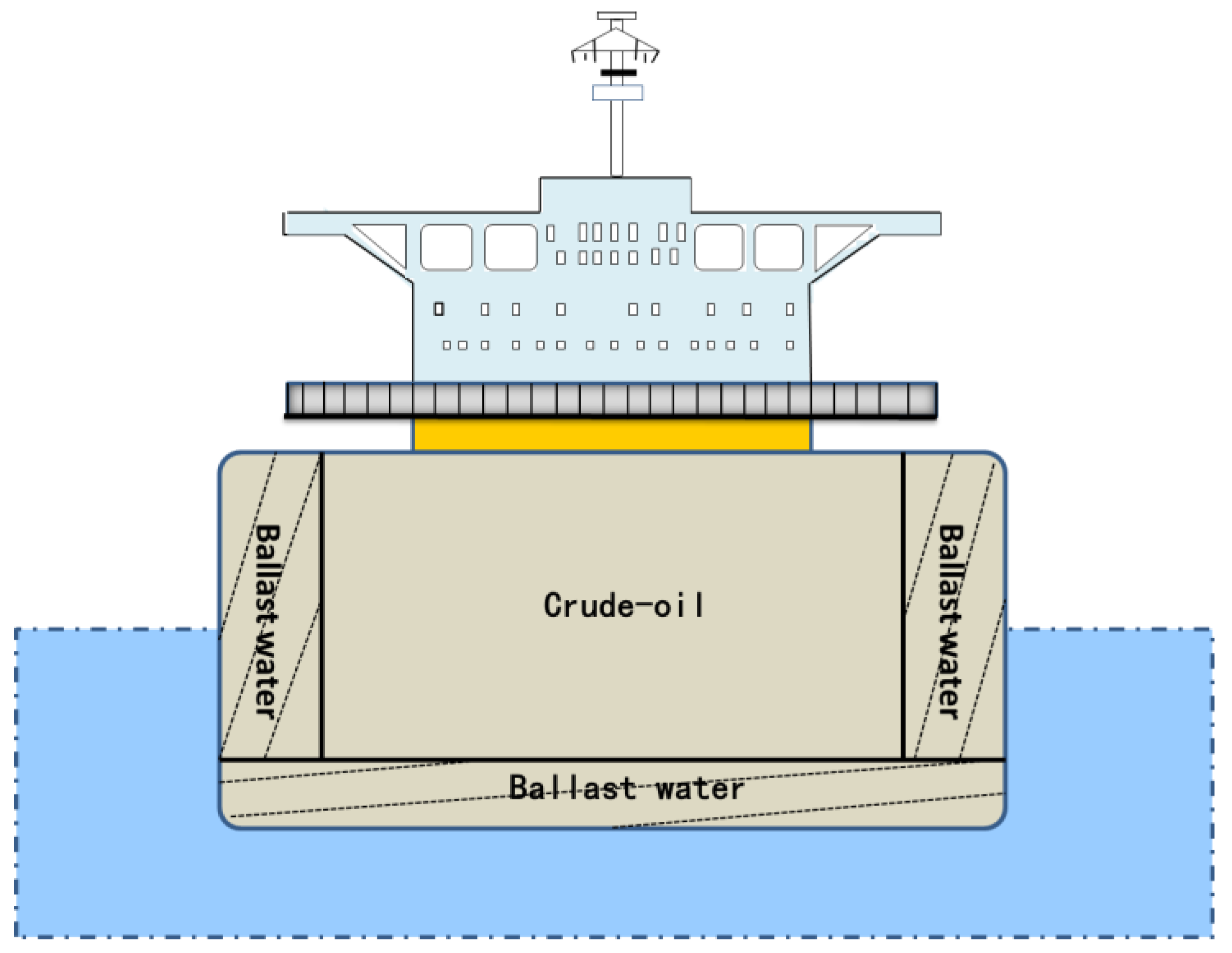
Modern large oil tankers are usually double hull vessels, with special ballast tanks at the sides of cargo tanks. The cross section of the tanker holds is shown as Figure 2. When the ship is sailing in ballast, the heat of crude oil in the tank is released to the sea through the inside shell, ballast water and outer shell. When the ship is not sailing in ballast, the heat of crude oil in the tank is released to the sea through the shell, the air and the shell. In addition, the crude oil in the tank exchanges heat with the inert gas at the top of the tank by convection. The inert gas occupies a small part of the oil tank, and the heat of the inert gas is released to the atmosphere through the upper deck. A heating coil is installed at the bottom of the cabin to avoid the oil temperature naturally cooling below freezing point due to the influence of the above factors. Considering the economy and practicability, the crude oil in the tank is heated to a temperature which is 10 °C above the gel point.
Since the temperature gradient of the crude oil in the longitudinal direction is very small, and the temperature gradient in the transverse direction is very large, the three-dimensional physical model is simplified to a two-dimensional one. This paper focuses on studying the influence of oscillating motion on the thermal and hydraulic characteristic of crude-oil, so the ballast water tank and inert gas tank are not considered. In addition, to save computation time, we only study a 40 cm × 30 cm model tank cargo. As mentioned above, the physical model of the thermal and hydraulic process of the crude oil in the tank cargo is shown in Figure 3.
The red section in Figure 3 represents the crude oil, the blue part indicates the air above the crude oil, and there is a phase interface between the crude oil and the air. The upper boundary is the deck of the tanker, exposed to the air and is subjected to the third boundary condition. The left and right sides are two side walls of the ship respectively, the lower part is immersed in the sea water, and the upper part is exposed to the air. Thus, the left and right boundaries are also subjected to third boundary condition. The lower boundary is the bottom of the ship and immersed in sea water, which is subjected to the third boundary condition. When the oil tanker is subjected to an oscillating motion, it is assumed that the tanker rotates with an imagined z axis which is perpendicular to x and y axis at the original point o of the coordinate system in Figure 3. To simplify calculations, the following assumptions are introduced:
- (1)
- The liquid oil does not evaporate, and the total volume does not change with temperature and time.
- (2)
- The oil tanker is only subjected to rotational motion.
- (3)
- The change of density with temperature is described by the Boussinesq approximation in the momentum equation, while the change of other physical properties with temperature is not considered, i.e., only the average value in the range of temperature change is used.
- (4)
- There is no phase change in the crude oil during temperature drop.
2.2. Mathematical Model
2.2.1. Governing Equations
The nature of the physical problem studied in this paper is the mixed convection heat transfer under external disturbances, so the governing equation is a convection diffusion equation. Since the computation domain is changing its position all the time, the governing equations is provided in the framework of dynamic grid system.
(1) Volume Fraction Equation
The tracking of the interface between the phases is accomplished by solution of a continuity equation for the volume fraction of one of the phases. For the qth phase, this equation has the following form:
In Equation (1), denotes the volume fraction of qth phase in the cell; is the velocity of qth phase, m/s; indicates the mass transfer from phase to phase , kg/(m3·s); and is the source term and is zero in this research, kg/(m3·s). The volume fraction equation is not solved for the primary phase; the primary-phase volume fraction is computed by .
The properties appearing in the transport equations are determined by the presence of the component phases in each control volume. In a gas–liquid system, if the phases are represented by the subscripts 1 and 2, and if the volume fraction of the second of these is being tracked, the density in each cell is given by
All other properties (for example, viscosity) are computed in this manner.
(2) Momentum conservation equation
where is the velocity of moving mesh, m/s; is static pressure, Pa; and is stress vector, Pa. is the volume-averaged velocity, m/s, which is calculated by
The density in the last term in Equation (3) is described by Boussinesq approximation, i.e., .
(3) Energy conservation equation
In Equation (5), volume-averaged value of h is calculated by
where h is the enthalpy, J/kg; is the effective conductivity, m2/s; and is the defined volume source term, W/m2.
Because of the oscillation, forced convection heat transfer will occur. Since the Reynolds number for a real-size oil tanker is large, the turbulence model should be employed for establishing a general mathematical model. In this paper, k-epsilon model is used to describe the turbulence effect. The equations of turbulent energy k and turbulent dissipation rate ε are as follows:
In these equations, is turbulent viscosity (), Pa·s. represents the generation of turbulence kinetic energy caused by mean velocity gradients, kg/(m·s3). is the generation of turbulence kinetic energy brought by buoyancy, kg/(m·s3). , , and are constants. and are the turbulent Prandtl numbers for and , respectively.
With respect to dynamic meshes, the integral form of the conservation equation for a general scalar, , on an arbitrary control volume, , whose boundary is moving can be written as
where is the diffusive coefficient, m2/s; is the source term of ; and indicates the boundary of control volume .
2.2.2. Boundary Conditions
As indicated in Figure 3, all the boundaries are subjected to the third-type boundary condition. The temperature of sea water is set to be 290.4 K, which is the annual average temperature of sea water; the temperature of air is chosen to be 293 K, which is also the annual average temperature. The initial temperature of the crude oil in the cabin is set at 323 K. It is provided in [17] that the forced heat transfer coefficient of water is 1000–1500 W/(m2·K), and that of air is 20–100 W/(m2·K). In this paper, the forced heat transfer coefficient of water is 1250 W/(m2·K), and that of air is 50 W/(m2·K). In conclusion, the detailed information about the boundary conditions is provided in Table 1.
3. Numerical Method
The computational domain is mapped by structured quadrilateral mesh generated by ICEM (The Integrated Computer Engineering and Manufacturing code) combined in ANSYSY FLUENT 15.0 [18], and the grid system is sketched in Figure 4. The rational grid density, which is 200 × 150, is determined after grid independent testing shown in Figure 5.
The governing equations are discretized in the framework of the finite volume method. The convection terms are discretized with the QUICK scheme. The volume fraction is discretized by QUICK scheme. The unsteady term is discretized by the first order forward difference. The coupling between velocity and pressure is calculated by semi-implicit pressure correction algorithm (SIMPLE algorithm). Since the problem studied involves the motion of the region and the free surface, the time step is set as 0.01 s. The discretized equations were solved by ANSYS FLUENT 15.0 solver.
Since the computational domain is changing its position with time, so a dynamic mesh technique is used in this research. The movement of the grid system is defined by a user defined function (DEFINE_CG_MOTION).
4. Results and Discussion
In this section, the temperature drop characteristic of the crude oil in the cargo tank at different oscillating frequencies is studied. To save computation time, only a small-size model tank cargo, which is 40 cm × 30 cm, is studied and shown in Figure 3. The depth of the crude oil is 22.5 cm (i.e., the thickness of air layer is 7.5 cm). The initial temperature in the tank cargo is 323.15 K uniformly. The physical properties of crude oil and air in the calculation are shown in Table 2. Non-Newtonian behavior of crude oil is not considered in this research, if anyone who wants to include this behavior, a power law [19] can be applied to characterize the non-Newtonian behavior of crude oil. With the parameters provided, the maximum Raleigh number for the static case can be calculated, which is 5 × 10⁸.
In this study, three different cases named Case 1, Case 2 and Case 3 will be tested for clarifying the influence of the oscillation on the temperature drop. The variables of the three cases are the rotational angular velocity. In Cases 1, the rotational angular velocity is 0, i.e., the tanker does not oscillate. In Cases 2 and 3, the rotational angular velocity is described by Equation (10).
In Equation (9), is the angular velocity of the oscillation motion, and varies by cosine. The period of angular velocity is the same as that of the tanker oscillation (); A and B are both constants. The amplitude of the tanker wobble can be calculated by , and can be obtained with and substituted. In the two oscillating cases, the time cycles of Case 2 and Case 3 are and , respectively. Therefore, in Equation (9) gives and , respectively. In the two oscillating cases, the amplitudes are equal, . Thus, in Equation (9), the values of are and respectively.
For easy reference, the information for Case 1 to Case 3 is listed in Table 3.
Under the above-mentioned calculation conditions, the thermal and hydraulic processes of the crude oil in the tanker cargo in three cases are calculated numerically. The hydraulic characteristics (including liquid surface movement and stream function) and the thermal characteristics (including boundary Nusselt number [20] and temperature field evolution) are investigated in detail. Afterwards, the sensitivity of temperature drop to rolling frequency is analyzed.
Figure 6 and Figure 7 show the gas liquid phase distribution at different time instants for Case 1 (static) and Case 2 (oscillation), respectively. In Case 1, the interface of gas–liquid phase does not change with time, and the phase distribution at different time is shown in Figure 6. Different from Case 1, the interface of the gas–liquid phase in oscillating case changes with time. Figure 7 shows the four typical time instants in Case 2 (). As shown in the figure, there is a small amount of wave on the surface at the beginning of the oscillation, and the liquid level tends to the horizontal surface as time goes by. This is because the oscillation frequency is small and the liquid surface has enough time to return to the horizontal plane.
Figure 8 shows four typical instantaneous stream functions in Case 1. As can be seen from the figure, the stream function is basically symmetrical. There are local vortices generated by natural convection at different position of the fluid region. There are two opposite vortices in the crude oil region, which are generated by natural convection on the left lower boundary and the right lower boundary. There are also a few pairs of vortices in the air region above the liquid level. In this static case, the flow field is dominated by local natural convection at different position.
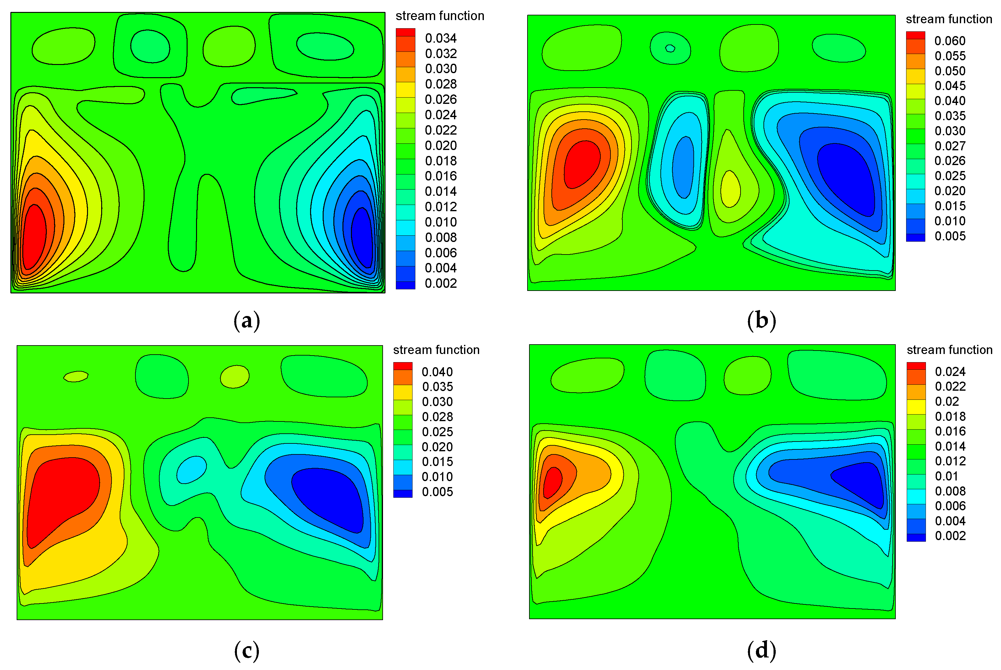
Figure 9 presents four typical instantaneous stream functions in Case 3, in which Figure 9a,b shows two states at which the domain is rotating to the left, and Figure 9c,d, shows two states at which the domain is rotating to the right. Different from Case 1, the flow field in Case 3 is dominated by integral flow generated by rotation. Because of the effect of rotation, the distribution of stream function is asymmetric, running towards the direction of rotation, and the direction of the flow is also alternately changing. In Figure 9, under the oscillating effect, the streamlines near the solid boundary are running consistent with the solid boundary trend, while there is a central vortex in the core area of the fluid.
To clarify the thermodynamic characteristics, the Nu distributions on the four boundaries are studied in this part. Figure 10 shows the Nu distributions on the four boundaries of the four typical time instants in Case 1. It can be seen from the figure that the left and right boundary have the identical Nu; and the Nu on the lower part of left and right boundaries is larger than that on the upper part, since the lower boundary immersed in the water and the upper part exposed in the air, and thus the convective coefficient between sea water and solid wall is larger than that between air and solid wall. On the lower boundary, Nu is larger in the middle and lower on both sides. As time proceeds, the Nu decreases significantly, and eventually tends to be stable. For the upper boundary, because there are pairs of vortices in the air region, the Nu of the upper boundary shows a wavy distribution. In general, the Nu on different boundaries gradually decreases with time. In the static case, the heat in the crude oil is mainly lost from the lower part of the left and right boundaries.
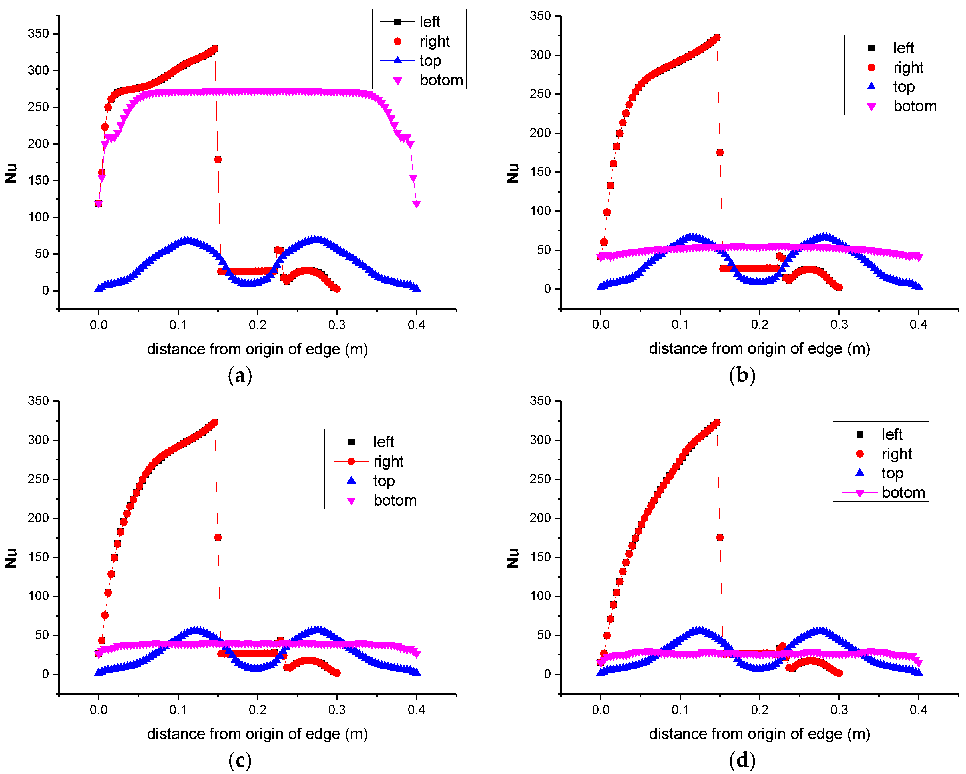
Figure 11 shows the Nu distribution on four boundaries at different instances in Case 3. Different from Figure 10, the length of the part immersed in the sea water varies during oscillation in Case 3, so the Nu distributions around the left and right boundaries are different and the distribution characteristic change with oscillation. With the oscillation, the flow field is in a complex change, so there is no clear characteristic on the Nu difference between the left and right boundaries. The Nu of the upper boundary is the smallest, and the Nu on the left, right and the lower boundaries are larger. As time proceeds, the Nu on each boundary decreases slightly. Unlike the static case, the Nu on the lower boundary does not decrease very much. The reason is that oscillation causes the fluid to move along the solid wall all the time, while, in Case 1, the flow near the lower boundary is very weak after a period of temperature drop. Thus, it can be concluded that the loss of heat from the left, right and lower boundary is greater, and that from the upper boundary is relatively small, for the oscillation situation.
Based on the analysis of hydraulic characteristics, the thermal process of the system is investigated. Figure 12 shows the temperature distribution at four typical time instants in the Case 1 (stationary condition). It is found that the temperature field is symmetrical. With the decrease of temperature, the temperature field of the crude oil shows stratified distribution that the lower part has a lower temperature and the upper part has a high temperature. This is the typical stratified temperature distribution formed by the natural convection of the crude oil in the tank. The temperature distribution in the air region presents a vortex distribution. This is because the natural convection of air causes the upper cold air to sink, while the hot air near the oil surface rises and transfers heat upwards. The air zone has multiple adjacent vortices in opposite directions.
The oscillation converts the natural convection in the stationary condition to a mixed convection, and thus the temperature drop characteristic changes dramatically. Figure 13 shows the temperature field distribution at four representative time instants in case 3 (). As can be seen in Figure 13, due to the role of oscillation, the temperature field presents an asymmetric distribution, and the temperature field has a tendency to shift toward the rotation. In the early phase of temperature drop, the temperature of the crude oil shows an approximately uniform distribution, and the temperature drop is very slight. However, the temperature drop in the air zone is obvious, and the oscillation makes the temperature distribution in the air zone asymmetric. With the decrease of temperature, the temperature near the four boundaries decreases rapidly, and the low-temperature zone expands gradually to the center. The oil temperature shows the phenomenon that the middle center is higher and the circumference is lower.
Comparing Figure 12 and Figure 13, it is found that the oscillation changes the temperature field, and the temperature field shifts to the direction of rotation. From the temperature data, the temperature drop rate under oscillating condition is generally higher than that for the static condition, and the greater the oscillating frequency, the greater the temperature drop rate. The quantitative contrast is shown in Figure 14.
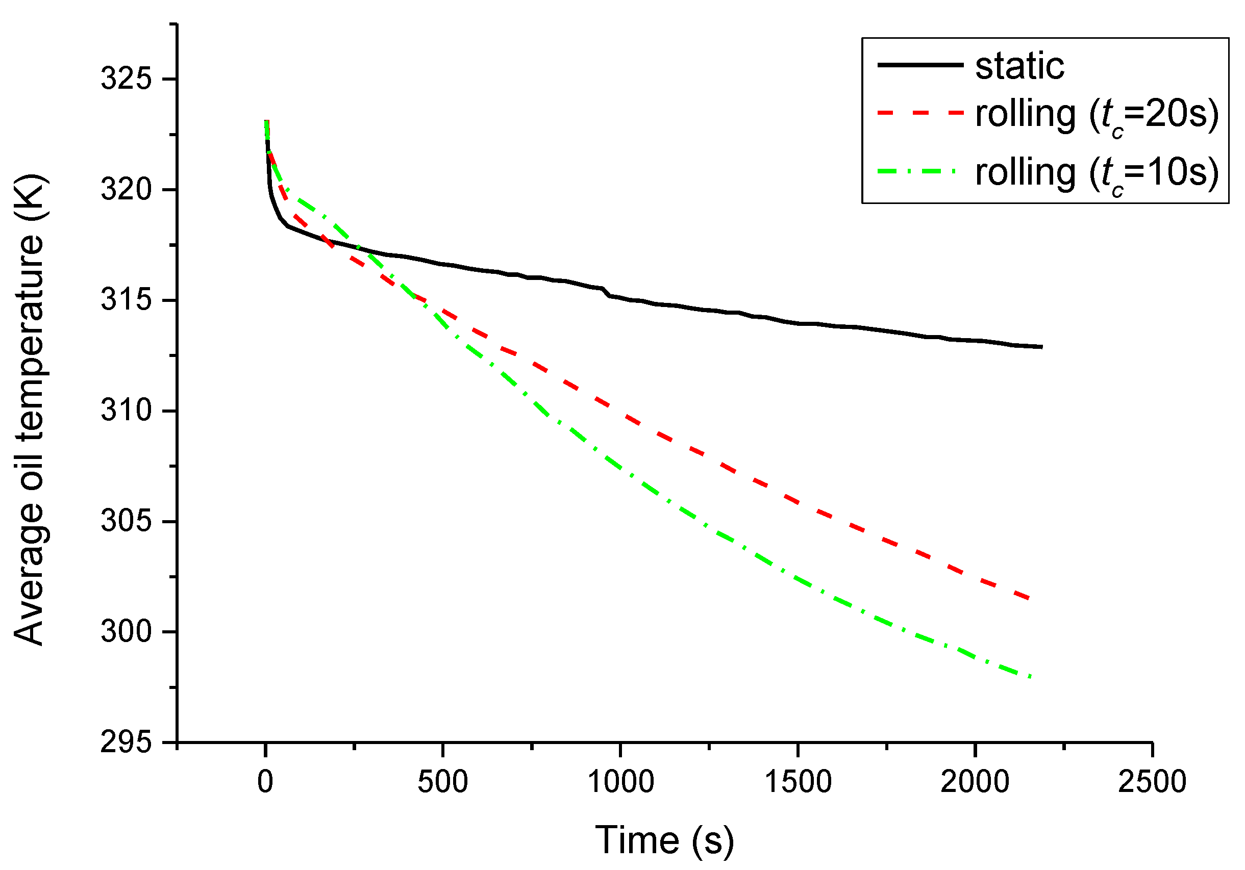
Figure 14 compares the average temperature changes versus time in the cargo in Case 1 (static), Case 2 () and Case 3 (). The temperature drop is obviously enhanced by the oscillating, and the larger the oscillating rate (i.e., the smaller the time cycle), the greater the temperature drop rate. This is because temperature drop of the crude oil under the stationary condition mainly depends on the natural convection, but, in oscillating condition, it depends on mixed convection (natural convection + forced convection), which enhances the heat transfer effect.
Since a small-size model oil tanker is discussed in this research, the thermal process will change if the size of the tanker is changed. If the size is increased to the real size, the Reynolds number, which is defined as , and the Grashof number, which is defined by , will increase dramatically. The Reynolds number and the Grashof number determine the strength of the forced convection and natural convection, respectively. Thus, the larger the tanker size, the more the oscillation will affect the thermal process.
5. Conclusions
In this paper, the thermal and hydraulic characteristic of the crude oil in the cargo tanker under the oscillating condition is numerically studied, with consideration of the free liquid surface motion under oscillating condition. The following conclusions are obtained:
(1) In the case of oscillation, the temperature drop process of crude oil is dominated by mixed convection. The temperature drop process is greatly enhanced and the temperature drop rate is remarkably increased compared with the natural convection for the static case.
(2) According to the actual oscillating period of the tanker, the wave of free surface is not obvious, and the horizontal liquid surface distribution is dominant.
(3) The larger is the oscillation frequency (i.e., the smaller the cycle), the greater is the temperature drop rate.
(4) For the static case, the heat in the crude oil is mainly lost from the lower part of the left and right boundaries, while, in the oscillating case, the loss of heat from the left, right and lower boundary is greater, and that from the upper boundary is relatively small.
Since only a 2D simplified model is studied in this research, future work will be focused on the real 3D model. In addition, the translational motion should be included in the future work as well.
Author Contributions
G.Y. conceived and designed the research case; Z.F. established the numerical model and performed the numerical simulation; B.D. and D.L. analyzed the solution data; Q.Y. wrote the paper.
Acknowledgments
The study is financially supported by National Science Foundation of China (Nos. 51606117 and 51606114), and China Postdoctoral Science Foundation funded project (2017M621473).
Conflicts of Interest
The authors declare no conflicts of interest
References
- Sun, X.; Qian, X.; Jiang, X. Report on the Development in Domestic and Foreign Oil and Gas Industry in 2015; Petroleum Industry Press: Dongying, China, 2016. [Google Scholar]
- BP. BP Energy Outlook, 2017 Ed.; BP p.l.c.: Orlando, FL, USA, 2017; Available online: http://www.bp.com/content/dam/bp/pdf/energy-economics/energy-outlook-2017/bp-energy-outlook-2017.pdf (accessed on 25 January 2017).
- Yin, J.; Tang, B. Analysis of Influence Factors in China Oil Imports Security. China Energy 2016, 11, 29–33. [Google Scholar]
- Li, H. Discussion on current situation and Countermeasures of crude oil transportation market in China. Chem. Eng. Equip. 2015, 6, 211–212. [Google Scholar]
- Yue, D. Calculation of Optimum Heating Time of Tanker Cargo Oil. In Excellent Collection of Academic Exchange Conference in 2006; China Institute of Navigation: Beijing, China, 2007; pp. 25–30. [Google Scholar]
- Zhang, C. Study on Heat Transfer Mechanism of Crude Oil Heating and Heat Preservation Process. Master’s Thesis, Dalian Maritime University, Dalian, China, 2007. [Google Scholar]
- Zhang, C.; Liang, Y.; Li, K.; Yue, D. The influence of steam parameters on the heating economy of cargo oil. J. Dalian Marit. Univ. 2005, 4, 38–40. [Google Scholar]
- Zhang, K. Development of Operation System for Oil Heating Process of Tanker. Master’s Thesis, Dalian Maritime University, Dalian, China, 2008. [Google Scholar]
- Shi, J.; Yin, P.; Zhang, L. Numerical calculation of temperature field in tanker cargo. J. Dalian Marit. Coll. 1989, 3, 69–74. [Google Scholar]
- Jin, Z. Research on Heating and Insulation Process of Tanker Cargo Based on FLUENT Platform. Master’s Thesis, Dalian Maritime University, Dalian, China, 2006. [Google Scholar]
- Akagi, S. Studies on the Heat Transfer of Oil Tank Heating of a Ship. J. Kansai Soc. Nav. Arch. Jpn. 1967, 124, 26–36. [Google Scholar]
- Suhara, J. Studies of heat transfer on tank heating of tankers. Jpn. Shipbuild. Mar. Eng. 1970, 5, 5–16. [Google Scholar]
- Chen, B.C.M. Cargo oil heating requirements for and FSO vessel conversion. Mar. Technol. 1996, 33, 58–68. [Google Scholar]
- Kato, H. Effects of Rolling on the Heat Transfer from Cargo Oils of Tankers. J. Soc. Nav. Arch. Jpn. 2009, 126, 421–430. [Google Scholar]
- Doerffer, S.; Mikielewicz, J. The influence of oscillations on natural convection in ship tanks. Int. J. Heat Fluid Flow 1986, 7, 49–60. [Google Scholar] [CrossRef]
- Akagi, S.; Kato, H. Numerical analysis of mixed convection heat transfer of a high viscosity fluid in a rectangular tank with rolling motion. Int. J. Heat Mass Transf. 1987, 30, 2423–2432. [Google Scholar] [CrossRef]
- Yang, S. Heat Transfer, 4th ed.; Higher Education Press: Beijing, China, 2006. [Google Scholar]
- Fluent, A. ANSYS Fluent Theory Guide 15.0; ANSYS, Inc.: Canonsburg, PA, USA, 2013. [Google Scholar]
- Huang, Z.; Zhang, X.; Yao, J.; Wu, Y.; Yu, T. Non-Darcy displacement by a non-Newtonian fluid in porous media according to the Barree-Conway model. Adv. Geo-Energy Res. 2017, 1, 74–85. [Google Scholar] [CrossRef]
- Luo, L.; Tian, F.; Cai, J.; Hu, X. The convective heat transfer of branched structure. Int. J. Heat Mass Transf. 2018, 116, 813–816. [Google Scholar] [CrossRef]
Figure 1.
Schematic of tanker navigation at sea.

Figure 2.
Schematic of the transverse section of a tanker.

Figure 3.
The physical model of the tank cargo system.

Figure 4.
Schematic of the grid system.

Figure 5.
Grid-independence test with Case 3.

Figure 6.
Instantaneous phase distribution in Case 1 (non-oscillation case).

Figure 7.
Instantaneous phase distribution in Case 2: (a) t = 1 s; (b) t = 18 s; (c) t = 42 s; and (d) t = 59 s.
Figure 7.
Instantaneous phase distribution in Case 2: (a) t = 1 s; (b) t = 18 s; (c) t = 42 s; and (d) t = 59 s.

Figure 8.
Instantaneous steam function in Case 1: (a) t = 60 s; (b) t = 660 s; (c) t = 1020 s; and (d) t = 2106 s.
Figure 8.
Instantaneous steam function in Case 1: (a) t = 60 s; (b) t = 660 s; (c) t = 1020 s; and (d) t = 2106 s.

Figure 9.
Instantaneous steam function in Case 3: (a) t = 264 s (moving to the left); (b) t = 660 s (moving to the left); (c) t = 990 s (moving to the right); and (d) t = 2112 s (moving to the right).
Figure 9.
Instantaneous steam function in Case 3: (a) t = 264 s (moving to the left); (b) t = 660 s (moving to the left); (c) t = 990 s (moving to the right); and (d) t = 2112 s (moving to the right).

Figure 10.
Instantaneous boundary Nusselt number in Case 1: (a) t = 60 s; (b) t = 660 s; (c) t = 1020 s; and (d) t = 2106 s.
Figure 10.
Instantaneous boundary Nusselt number in Case 1: (a) t = 60 s; (b) t = 660 s; (c) t = 1020 s; and (d) t = 2106 s.

Figure 11.
Instantaneous boundary Nusselt number in Case 3: (a) t = 264 s (moving to the left); (b) t = 660 s (moving to the left); (c) t = 990 s (moving to the right); and (d) t = 2112 s (moving to the right).
Figure 11.
Instantaneous boundary Nusselt number in Case 3: (a) t = 264 s (moving to the left); (b) t = 660 s (moving to the left); (c) t = 990 s (moving to the right); and (d) t = 2112 s (moving to the right).

Figure 12.
Instantaneous temperature fields in Case 1 (non-osculating condition): (a) t = 1 s; (b) t = 20 min; (c) t = 40 min; and (d) t = 60 min.
Figure 12.
Instantaneous temperature fields in Case 1 (non-osculating condition): (a) t = 1 s; (b) t = 20 min; (c) t = 40 min; and (d) t = 60 min.

Figure 13.
Instantaneous temperature fields in Case 3: (a) t = 60 s (The tanker is rotating to the left); (b) t = 682 s (The tanker is rotating to the left); (c) t = 992 s (The tanker is rotating to the right); and (d) t = 2108 s (The tanker is rotating to the right).
Figure 13.
Instantaneous temperature fields in Case 3: (a) t = 60 s (The tanker is rotating to the left); (b) t = 682 s (The tanker is rotating to the left); (c) t = 992 s (The tanker is rotating to the right); and (d) t = 2108 s (The tanker is rotating to the right).

Figure 14.
Comparison of average temperature drop under different rolling frequency.


Table 1.
Boundary conditions.
| Boundaries | Convective Heat Transfer Coefficient | Fluid Temperature |
|---|---|---|
| , | ||
| , | ||
| , | ||
| , | ||
| , |
Table 2.
Physical properties of crude oil and air.
| Materials | Density (kg/m3) | Thermal Conductivity (W/m·°C) | Specific Heat Capacity (J/kg·°C) | Dynamic Viscosity (Pa·s) | Volume Expansion Coefficient (1/°C) |
|---|---|---|---|---|---|
| crude oil | 850 | 0.14 | 2000 | 0.004 | 1.0 × 10⁻⁵ |
| air | 1.225 | 0.0242 | 1006.43 | 1.7894 × 10⁻⁵ | 0.00272 |
Table 3.
Information for the three test cases.
| Case | Time Cycle of Oscillation | Amplitude of Oscillation |
|---|---|---|
| Case 1 | ∞ | 0 |
| Case 2 | 10 s | |
| Case 3 | 20 s |
© 2018 by the authors. Licensee MDPI, Basel, Switzerland. This article is an open access article distributed under the terms and conditions of the Creative Commons Attribution (CC BY) license (http://creativecommons.org/licenses/by/4.0/).
Share and Cite
MDPI and ACS Style
Yu, G.; Yang, Q.; Dai, B.; Fu, Z.; Lin, D. Numerical Study on the Characteristic of Temperature Drop of Crude Oil in a Model Oil Tanker Subjected to Oscillating Motion. Energies 2018, 11, 1229. https://doi.org/10.3390/en11051229
AMA Style
Yu G, Yang Q, Dai B, Fu Z, Lin D. Numerical Study on the Characteristic of Temperature Drop of Crude Oil in a Model Oil Tanker Subjected to Oscillating Motion. Energies. 2018; 11(5):1229. https://doi.org/10.3390/en11051229
Chicago/Turabian StyleYu, Guojun, Qiuli Yang, Bing Dai, Zaiguo Fu, and Duanlin Lin. 2018. "Numerical Study on the Characteristic of Temperature Drop of Crude Oil in a Model Oil Tanker Subjected to Oscillating Motion" Energies 11, no. 5: 1229. https://doi.org/10.3390/en11051229
Note that from the first issue of 2016, this journal uses article numbers instead of page numbers. See further details here.