Local Stability Analysis and Controller Design for Speed-Controlled Wind Turbine Systems in Regime II.5


1
Munich School of Engineering, Research Group “Control of Renewable Energy Systems”, Technical University of Munich, Lichtenbergstraße 4a, 85748 Garching, Germany
2
Faculty of Electrical Engineering and Information Technology, Munich University of Applied Sciences, Lothstraße 64, 80335 München, Germany
*
Author to whom correspondence should be addressed.
Energies 2018, 11(5), 1251; https://doi.org/10.3390/en11051251
Submission received: 27 March 2018
/
Revised: 7 May 2018
/
Accepted: 11 May 2018
/
Published: 14 May 2018
(This article belongs to the Section L: Energy Sources)
Abstract
:The paper presents a local stability analysis for machine speed control of wind turbine systems (WTS) in regime II.5, where the control objective is set-point reference tracking of the machine speed via a PI-controller. Stability criteria for the controller parameters are derived. Based on these criteria, the controller parameters are chosen by pole placement. Moreover, a model-based tuning rule is proposed which leads (i) to a stable and (ii) to an accurate and fast control performance. The control system is additionally augmented by anti-windup (AWU) and saturation (SAT) strategies to enhance its performance. Simulation results illustrate stability and tracking performance of the closed-loop system.
1. Introduction
The increasing amount of wind power for electrical power generation (% in Germany 2016 [1], p. 7) necessitates a detailed understanding of wind turbine systems (WTS) to be capable of fulfilling the increasing requirements [2] (e.g., more strict grid codes) for wind turbine operators.
This paper discusses machine speed control of WTS in regime II.5. Figure 1 shows the (simplified) dependence of machine speed reference (in ) on the wind speed (in ) for different operation regimes (for details see e.g., [3,4,5]). Each regime has its own machine speed control system. In regime I, the wind speed is too small to achieve an economic operation of the WTS, whereas, in regime IV, the wind speed is too high and would overload the mechanical structure of the WTS [6]. Hence, in both regimes, the WTS is not operated. In regime I, it is freely floating (without active speed control) to be ready to start its operation as soon as the wind speed exceeds the cut-in wind speed (transition to regime II). In regime IV, the WTS is usually at standstill for safety reasons.
In regime II, the machine speed (in ) is controlled by a nonlinear controller (see e.g., [7,8]) to achieve an optimal and constant ratio . This ensures maximal power generation in regime II (i.e., maximum power point tracking, for details see [6,7,8]). In regime II.5, the machine speed is limited by some (in ) to reduce e.g., acoustic noise (when the WTS is close to buildings). But, then, since nominal power is not yet reached, the machine torque (in ) and, hence, the output power can still be increased [9]. Regime III is characterized by a limitation of both, machine speed and machine torque . In this regime, the pitch angle (in ) controls the machine speed and compensates for the increasing wind speed and wind power (in ) (see e.g., [10,11]).
This paper focuses on regime II.5. In [12,13], it is explained that reasons for the machine speed limitation are, e.g., “acoustic noise, loads or other design constraints” ([12], p. 488). In regime II.5, neither the nonlinear controller of regime II (see e.g., [6,7]) nor the pitch controller of regime III (see e.g., [2], Chapter 25) can achieve the goals of machine speed control in regime II.5: (a) tracking of the constraint machine speed reference and (b) maximized power generation of the WTS. A simple method to achieve (a) is “to implement a torque-speed ramp” [13], which is explained in detail in [13,14]. This method has several drawbacks; e.g., the WTS does not operate at its maximally achievable power generation and the “torque demand will be varying rapidly up and down the slope” ([12], p. 489). To overcome these drawbacks, ref. [15] proposes the use of a simple PI-controller, where the (optimal) reference torque (in ) is the controller output. Besides the benefit that a PI-controller is a state-of-the-art controller and widely spread in industry, the use of the PI-controller achieves both goals (a) & (b), and, additionally, is able to produce only small torque variations (see [12], p. 489). Therefore, in the following, a PI-controller will be considered to control the machine speed via the machine torque in regime II.5. To the best knowledge of the authors, there does not exist a (local) stability analysis and model-based tuning rule for a speed PI-controller in regime II.5.
This paper analysis the dynamical system (including mechanical system, speed control system with PI-controller and underlying torque control loop) of a WTS in regime II.5. It will be shown that a bad controller parameter design will cause instability of the closed-loop system. To avoid that, model-based stability criteria for a stable closed-loop system are derived. Based on these criteria, a tuning rule for the controller parameters is proposed which (i) guarantees (local) stability of the closed-loop system and (ii) leads to an accurate and fast tracking of the machine speed reference . Moreover, additional anti-windup (AWU) and saturation (SAT) strategies are applied to enhance the control performance further.
The paper is organized as follows: Section 2 discusses the nonlinear dynamics of the system. These dynamics will be linearized via Taylor series expansion in Section 3. In Section 4 the (linearized) dynamics will be analyzed with respect to closed-loop system stability. Section 5 proposes a tuning rule for PI-controller parameter design including the AWU & SAT strategies. Finally, in Section 6, simulation results illustrate the theoretical results.
2. Dynamics of the System
Control objective is tracking of a machine speed reference in regime II.5 via a proportional-integral (PI) controller. For the analysis, the machine torque reference is considered as control input, i.e., the control law is given by
with proportional gain (in ), integral gain (in ) and integral state (in ). The dynamics of the integral state are
Hence, the tuning parameters are and which must be chosen carefully and properly to achieve a stable closed-loop system with good tracking performance. Stability analysis and controller design (tuning) are presented in Section 4 and Section 5, respectively.
2.1. Dynamics of the Mechanics
For the dynamics of the machine speed with initial value the following holds:
with total inertia (in ), turbine torque (in ), gear ratio (in 1), air density (in ), turbine radius (in ), wind speed (in ) and power factor curve (in 1) which depends on tip speed ratio (in 1) and pitch angle . (3) is a standard model of the machine speed dynamics in WTS and can e.g., be found in [16], ([17], Chapter 4).
2.2. Dynamics of the Underlying Control Loop of the Machine Torque
The capability to track the machine torque reference results from an underlying control loop of the machine torque (based on machine current control via a voltage source inverter and pulse-width modulation). The dynamics of the machine torque control are quite fast (compared to those of the mechanics) and are approximated via the first-order lag system (see e.g., [6])
with initial value , gain (in 1) and time constant . A well designed machine torque controller yields .
2.3. Overall Dynamics
By introducing state vector , disturbance vector , reference input and output , the overall (nonlinear) system dynamics can be written as
with .
3. Linearization
The dynamics of system (5) will be linearized via Taylor series expansion around the operation point . Hence, the following small-signal approximations are defined:
Applying the Taylor series expansion to system (5) yields
with initial values , and . The term characterizes the higher order terms of the Taylor series. Imposing the following
Assumption 1.
The higher order terms of the Taylor series are neglected, i.e.,
Allows to approximate the nonlinear system (5) by its small signal (linearized) dynamics
where system matrix , input vector and disturbance matrix are given by
and the following definition holds: .
4. Stability Analysis
In this section, based on the linearization above, a local stability analysis is performed. One obtains the following stability condition:
Condition 1.
Proof of Condition 1.
In view of Hurwitz’s theorem (see e.g., ([18], Chapter 8), ([19], Chapter 1)), system (7), (8) is stable, if and only if (a) and (b) hold. Clearly, because of , and , the inequalities and result in and of Condition 1. necessitates the condition which is already satisfied if holds, since
The term is given by
Remark 1.
A physical interpretation of Condition 1 is the following: must hold, since the integral gain has to act with correct sign. Moreover, the underlying machine torque control loop has to be faster than the outer control loop of the machine speed. This results in where the time constant of the torque control loop leads to an upper bound on for . characterizes the impact of integral and proportional gain on closed-loop stability.
Sub-conditions and depend on and, consequently, on the operation point . Since it is necessary that and are fulfilled for all possible operation points , the most critical operation point needs to be considered for the design of the controller parameters and (worst-case analysis). Figure 2a illustrates the sector of all feasible and which yield a (locally) stable closed-loop system (7), (8).
Condition 2.
For the critical operation point the following holds:
Thus, the maximal value of all possible is the most critical one.
Proof of Condition 2.
The calculation of the derivative of the right term of with respect to yields
Thus, the derivative in (15) is strictly negative and, accordingly, the greater the smaller is the right term of . Hence, for the most critical choice of , the inequalities and hold for any operation point. ☐
In regime II.5—where the PI-controller is used—the pitch angle is controlled to its optimal (but constant) value, i.e., . Consequently, in regime II.5, the following holds: . By defining the boundary with and , as illustrated in Figure 2b, the following holds:
Condition 3.
The set—where the critical operation point is located in—is given by
Proof of Condition 3.
In regime II.5, the set Λ of all possible operation points of the tip speed ratio results in with and . Hence, both and cover all (see Figure 2b). By taking and into account, is finally given by
Consequently, (17) is equivalent to (Condition 3). ☐
5. Controller Design
In this section, the stability condition is translated into a simple tuning rule for the PI-controller parameters.
5.1. Controller Parameter Tuning
The following tuning rule for the parameters and of the PI-controller is based on pole placement. The closed-loop poles of the (linearized) system (7), (8) are specified by some desired (real and negative) poles which leads to the desired polynomial
Note that the closed-loop poles of (7), (8) can not be chosen independently; since, comparing the coefficients of the characteristic and desired polynomial (see (9) and (18)) yields the following overdetermined equation system with three equations but only two free design parameters and :
To guarantee (local) stability for all possible operation points, the comparison of the coefficients in (19) is accomplished for the critical operation point . For the tuning of the parameters and , and (19) have to be fulfilled. Therefore, the following tuning rule
for and is proposed, where is a single free design parameter which assures local stability and can be adjusted to achieve good tracking performance.
Remark 2.
The choice of the control parameters and as in (20) gives the closed-loop poles and , which are clearly negative.
Proof of Remark 2.
Inserting the closed-loop poles of (Remark 2) into (19) yields
5.2. Anti-Wind Up and Saturation
To enhance the PI-controller control performance, it is augmented by an additional anti-wind up (AWU) and saturation (SAT) block as shown in Figure 3, where the following holds (the idea of (22) is taken from [20], Chapter 14):
where (in ) are the minimal/maximal machine torque available in regime II.5. (AWU) and (SAT) take the saturated (available) machine torque in regime II.5 into account in order to avoid (i) unfeasible torques and (ii) windup effects (which would deteriorate the tracking performance, see [20], Chapter 14).
6. Simulation Results
In this section, the theoretical findings are illustrated by simulation results for four different scenarios:
- Scenario 1: Control performance for a constant but maximal speed reference to illustrate stability and set-point tracking control performance.
- Scenario 2: Control performance for an arbitrarily time-varying speed reference to illustrate stability and reference tracking control performance at different operation points.
- Scenario 3: Control performance for a constant but maximal speed reference for three different controller tunings to illustrate the effect of tuning on stability and set-point tracking control performance.
- Scenario 4: Control performance for an arbitrarily time-varying speed reference for three different controller tunings to illustrate the effect of tuning on stability and reference tracking control performance at different operation points.
All scenarios are fed by the same realistic wind speed profile. The control performance of all four scenarios is evaluated by the integral absolute error (IAE) performance measure. The IAE performance measure is computed by [20]
Figure 3 shows the implementation block diagram of controller and physical system in Matlab/Simulink. Simulation data is collected in Table 1. The power factor of the WTS is approximated by (for details see [21])
with , and as in Table 1. Figure 4 depicts the power factor and additionally . For the critical operation point of the considered system, the following holds: .
Scenario 1:Figure 5 shows the simulation result for Scenario 1, where the machine speed is controlled to its maximal value, i.e., . To point out the impact of variations of the wind speed , real wind data (The authors are deeply grateful to the FINO-Project (BMU, PTJ, BSH, DEWI GmbH) for providing the wind data.) is used. The simulation illustrates the stable and good control performance of the controller design as in (20), since the control performance is characterized by an accurate tracking of the machine speed reference . The IAE value of verifies the accurate reference tracking (see Table 2). The right hand-side of Figure 5 shows the wind and turbine power (with ), the tip speed ratio and the power factor . As expected for regime II.5, the WTS operates below the optimal tip speed ratio and consequently does not reach the optimal power factor .
Scenario 2:Figure 6 illustrates the control performance under a time-varying machine speed reference , where significant changes in are allowed. Again, the control performance achieves an accurate and fast tracking of the machine speed reference with an IAE value of . The IAE value of this scenario is also small but larger than the IAE value of Scenario 1 due to the rapidly changing reference and the actuator constraint (SAT) which activates the anti-windup strategy as in (22). The machine torque reference is upper and lower bounded by and , respectively. Clearly, the jumps in the machine speed reference cause rapid changes in the machine torque and accordingly strong loads on the mechanical components. Since the normal operation in regime II.5 is characterized by a fixed (constant) machine speed reference , the peaks in the machine torque in Figure 6 at and would not occur and stress the mechanical components (as shown in Figure 5).
Scenario 3: To illustrate the impact of badly tuned controller parameters and on stability and set-point tracking control performance, Scenario 1 is repeated for three different controller tunings; see controller tunings (a), (b) & (c) in Table 2. The simulation results for Scenario 3 are shown in Figure 7: (a) — shows a stable but slow control performance. Even for the constant machine speed reference , the controller is not able to compensate for the changes in the wind speed and turbine torque . The IAE value of is much greater than the value of Scenario 1. The selected parameters of tuning (b) - - - violate sub-condition (ii) of the stability condition (Condition 1) whereas the selected parameters of tuning (c) ⋯ violate sub-condition (iii) of (Condition 1). Hence, for the cases (b) and (c), the closed-loop systems are unstable and their IAE values of and are extremely large (see Table 2).
Scenario 4: Scenario 4 is similar to Scenario 2 and uses a time-varying speed reference to illustrate the reference tracking control performance for different operation points. The simulation results are shown in Figure 8. The impact of the badly tuned controller parameters (a) —, (b) - - - and (c) ⋯ is obvious. The control performance of the stable but slow tuning (a) results in an IAE value of , which is not acceptable and even worse than that in Figure 7 (Scenario 3). Moreover, the tunings (b) - - - and (c) ⋯ yield again an unstable closed-loop system with extremely high IAE values of and , respectively.
7. Conclusions
The paper presented a local stability analysis for a machine speed PI-controller design for wind turbine systems operated in regime II.5. The proportional gain and integral gain of the PI-controller must be chosen properly to guarantee a (locally) stable closed-loop system. Therefore—based on the derived stability criteria—a tuning rule for the controller parameters via pole placement was proposed, which can achieve both: a stable closed-loop system and accurate and fast reference tracking. Four simulation scenarios have been implemented in Matlab/Simulink to demonstrate the achievable control performance of the proposed controller design and the effect of badly tuned controller designs on stability and tracking accuracy. The tracking control performance of all scenarios was compared and evaluated by the integral absolute error (IAE) performance measure. The simulation results showed that even, if the derived stability criteria is satisfied, a wrong controller tuning may give a slow and bad control performance leading to high IAEs values. Finally, the simulation results also demonstrated that, if the stability criteria is violated, then the closed-loop system becomes (as expected) unstable.
Author Contributions
C.D. derived and implemented the model, conducted the simulations, wrote the article and created the figures and plots; C.D. and C.M.H. analyzed and evaluated the simulation data; C.M.H. gave valuable advice in the modeling, helped writing the introduction, simulation and conclusion sections and revised the article.
Funding
This work was supported by the Technical University of Munich (TUM) in the framework of the Open Access Publishing Program.
Conflicts of Interest
The authors declare no conflict of interest.
Nomenclature
| Symbols | Description |
| , , | operation point, initial value, small signal approximation |
| , , | turbine power, turbine torque and turbine radius |
| , , , | wind power, air density, gear box ratio and total inertia |
| , , , , | machine speed, its reference, minimum, maximum and critical operation point |
| , , , | wind speed, its minimum, maximum and critical operation point |
| , | bounds the range of wind speeds, where the WTS is in operation |
| , , | pitch angle, its critical and optimal operation point |
| , , | machine torque, its minimum and maximum |
| , | machine torque reference and its saturated value |
| , , , , | tip speed ratio, its minimum, maximum and critical/optimal operation point |
| , , –, h | power factor, its optimum, coefficients and function of the power factor curve |
| , | gain and time constant of the underlying machine torque controller |
| , , | integral state, proportional gain and integral gain of the PI-controller |
| , , | design parameter and saturation function, higher order terms of Taylor appr. |
| , , v, y | state and disturbance vector, reference input and output of the system |
| , , , | system and disturbance matrix, input and output vector of the system |
| , , , | characteristic polynomial of the linearized system and its coefficients |
| , , , | desired characteristic polynomial of the controller design and its poles |
| := | dynamics of machine speed, machine torque and integral state |
| , , | derivative of in respect of machine speed, wind speed and pitch angle |
| , , | critical operation point of , functions to characterize |
| , , , , | operation sets of tip speed ratio and regime II.5, (parts of) boundary of |
References
- Durstewitz, M.; Berkhout, V.; Cernusko, R.; Faulstich, S.; Hahn, B.; Hirsch, J.; Kulla, S.; Pfaffel, S.; Rohrig, K.; Rubel, K.; et al. Windenergiereport Deutschland 2016; Technical Report; Fraunhofer-Institut für Windenergie und Energiesystemtechnik (IWES): Kassel, Germany, 2017. [Google Scholar]
- Ackermann, T. (Ed.) Wind Power in Power Systems; John Wiley & Sons, Ltd.: Chichester, UK, 2012. [Google Scholar]
- Gasch, R.; Twele, J. Windkraftanlagen—Grundlagen, Entwurf, Planung und Betrieb, 8th ed.; Vieweg + Teubner Verlag: Berlin/Heidelberg, Germany, 2013. [Google Scholar]
- Manwell, J.F.; McGowan, J.G.; Rogers, A.L. Wind Energy Explained: Theory, Design and Application; John Wiley & Sons: Hoboken, NJ, UAS, 2009. [Google Scholar]
- Quaschning, V. Regenerative Energiesysteme; Hanser Verlag: Munich, Germany, 2011. [Google Scholar]
- Dirscherl, C.; Hackl, C.; Schechner, K. Modellierung und Regelung von modernen Windkraftanlagen: Eine Einführung. In Elektrische Antriebe—Regelung von Antriebssystemen; Schröder, D., Ed.; Springer: Berlin/Heidelberg, Germany, 2015; Chapter 24; pp. 1540–1614. [Google Scholar]
- Pao, L.Y.; Johnson, K.E. Control of Wind Turbines: Approaches, Challenges, and recent Developments. IEEE Control Syst. Mag. 2011, 31, 44–62. [Google Scholar] [CrossRef]
- Mullen, J.; Hoagg, J.B. Wind turbine torque control for unsteady wind speeds using approximate-angular-acceleration feedback. In Proceedings of the 2013 IEEE 52nd Annual Conference on Decision and Control (CDC), Florence, Italy, 10–13 December 2013; pp. 397–402. [Google Scholar]
- Muller, S.; Deicke, M.; De Doncker, R.W. Doubly fed induction generator systems for wind turbines. IEEE Ind. Appl. Mag. 2002, 8, 26–33. [Google Scholar] [CrossRef]
- Slootweg, J.G.; de Haan, S.W.H.; Polinder, H.; Kling, W.L. General model for representing variable speed wind turbines in power system dynamics simulations. IEEE Trans. Power Syst. 2003, 18, 144–151. [Google Scholar] [CrossRef]
- Hand, M.M.; Balas, M.J. Systematic controller design methodology for variable-speed wind turbines. Wind Eng. 2000, 24, 169–187. [Google Scholar] [CrossRef]
- Burton, T.; Jenkins, N.; Sharpe, D.; Bossanyi, E. Wind Energy Handbook; John Wiley & Sons: Hoboken, NJ, UAS, 2011. [Google Scholar]
- Bossanyi, E.A. The design of closed loop controllers for wind turbines. Wind Energy 2000, 3, 149–163. [Google Scholar] [CrossRef]
- Bossanyi, E.; JENKINS, N. Electrical Aspects of Variable Speed Operation of Horizontal Axis Wind Turbine Generators; Technical Report, ETSU W/33/00221/REP; Energy Technology Support Unit: Harwell, UK, 1994. [Google Scholar]
- Bossanyi, E. Wind turbine control for load reduction. Wind Energy 2003, 6, 229–244. [Google Scholar] [CrossRef]
- Dirscherl, C.; Hackl, C.M. Dynamic power flow in wind turbine systems with doubly-fed induction generator. In Proceedings of the 2016 IEEE International Energy Conference (ENERGYCON), Leuven, Belgium, 4–8 April 2016; pp. 1–6. [Google Scholar] [CrossRef]
- Johnson, G.L. Wind Energy Systems. Electronic Edition, 2006. Available online: https://www.ece.k-state.edu/people/faculty/gjohnson/files/Windbook.pdf (accessed on 26 March 2018).
- Bhattacharyya, S.; Datta, A.; Keel, L. Linear Control Theory: Structure, Robustness, and Optimization; Automation and Control Engineering, CRC Press: Boca Raton, FL, USA, 2009. [Google Scholar]
- Ackermann, J. Robust Control: The Parameter Space Approach, 2nd ed.; Springer: London, UK, 2002. [Google Scholar]
- Hackl, C.M. Non-Identifier Based Adaptive Control in Mechatronics: Theory and Application; Number SPIN 86365067 in Lecture Notes in Control and Information Sciences; Springer: Berlin, Germany, 2017. [Google Scholar]
- Heier, S. Windkraftanlagen: Systemauslegung, Netzintegration und Regelung, 5th ed.; Vieweg + Teubner Verlag: Berlin/Heidelberg, Germany, 2009. [Google Scholar]
Figure 1.
Machine speed reference for different operation regimes in wind turbine systems (based on Figure 12-2 in [3]).
Figure 1.
Machine speed reference for different operation regimes in wind turbine systems (based on Figure 12-2 in [3]).
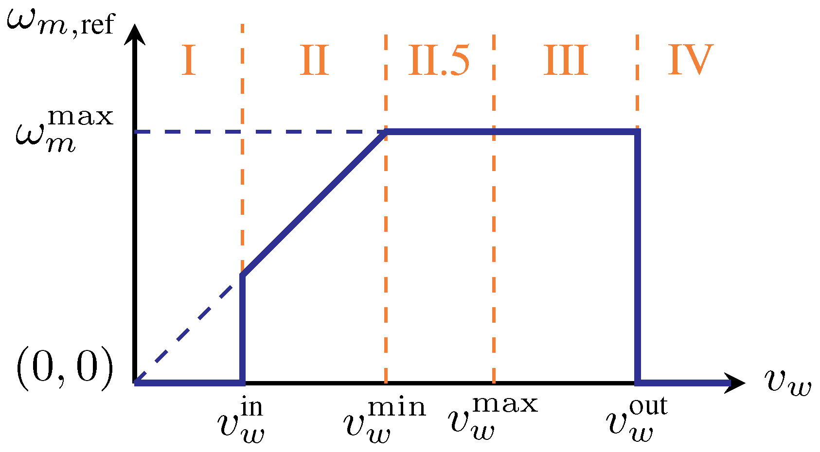
Figure 2.
Stability analysis and interpretation of the closed-loop system (7).
Figure 2.
Stability analysis and interpretation of the closed-loop system (7).
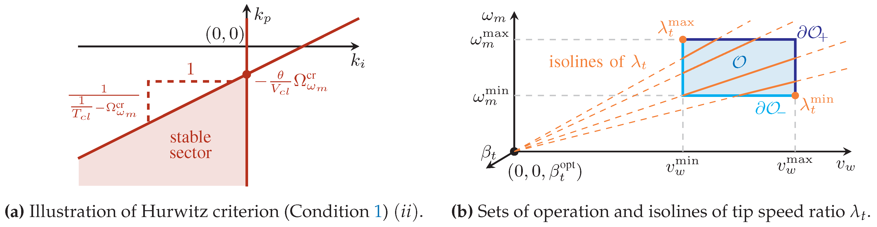
Figure 3.
Block diagram of implementation: PI-controller, SAT & AWU and physical system. A well-designed PI-controller with proportional gain and integral gain is essential to guarantee closed-loop stability (see Section 4 and Section 5).

Figure 4.
Illustration of power coefficient (left), the dependence of on wind speed and machine speed (middle) and on wind speed and tip speed ratio (right).
Figure 4.
Illustration of power coefficient (left), the dependence of on wind speed and machine speed (middle) and on wind speed and tip speed ratio (right).

Figure 5.
Simulation results for Scenario 1—set-point tracking control performance in regime II.5: Wind speed , machine speed , machine and turbine torque, wind and turbine power, tip speed ratio and power factor .
Figure 5.
Simulation results for Scenario 1—set-point tracking control performance in regime II.5: Wind speed , machine speed , machine and turbine torque, wind and turbine power, tip speed ratio and power factor .
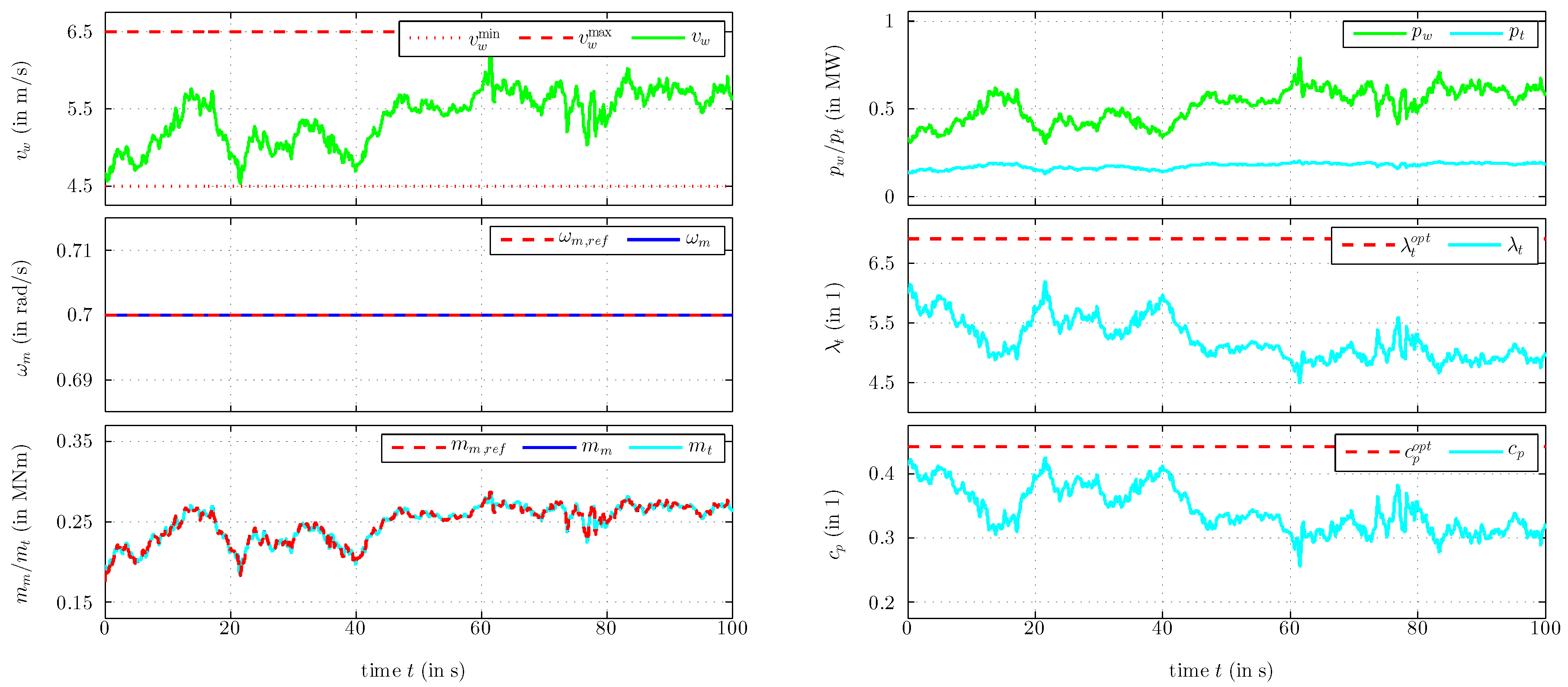
Figure 6.
Simulation results for Scenario 2—reference tracking control performance in regime II.5 ( is arbitrarily time-varying): Wind speed , machine speed , machine and turbine torque, wind and turbine power, tip speed ratio and power factor .
Figure 6.
Simulation results for Scenario 2—reference tracking control performance in regime II.5 ( is arbitrarily time-varying): Wind speed , machine speed , machine and turbine torque, wind and turbine power, tip speed ratio and power factor .

Figure 7.
Simulation results for Scenario 3—set-point tracking control performance in regime II.5 for three different controller tunings (a) — stable but slow tuning with and , (b) - - - unstable tuning with and , (c) ⋯ unstable tuning with and : Wind speed , machine speed , machine and turbine torque, wind and turbine power, tip speed ratio and power factor .
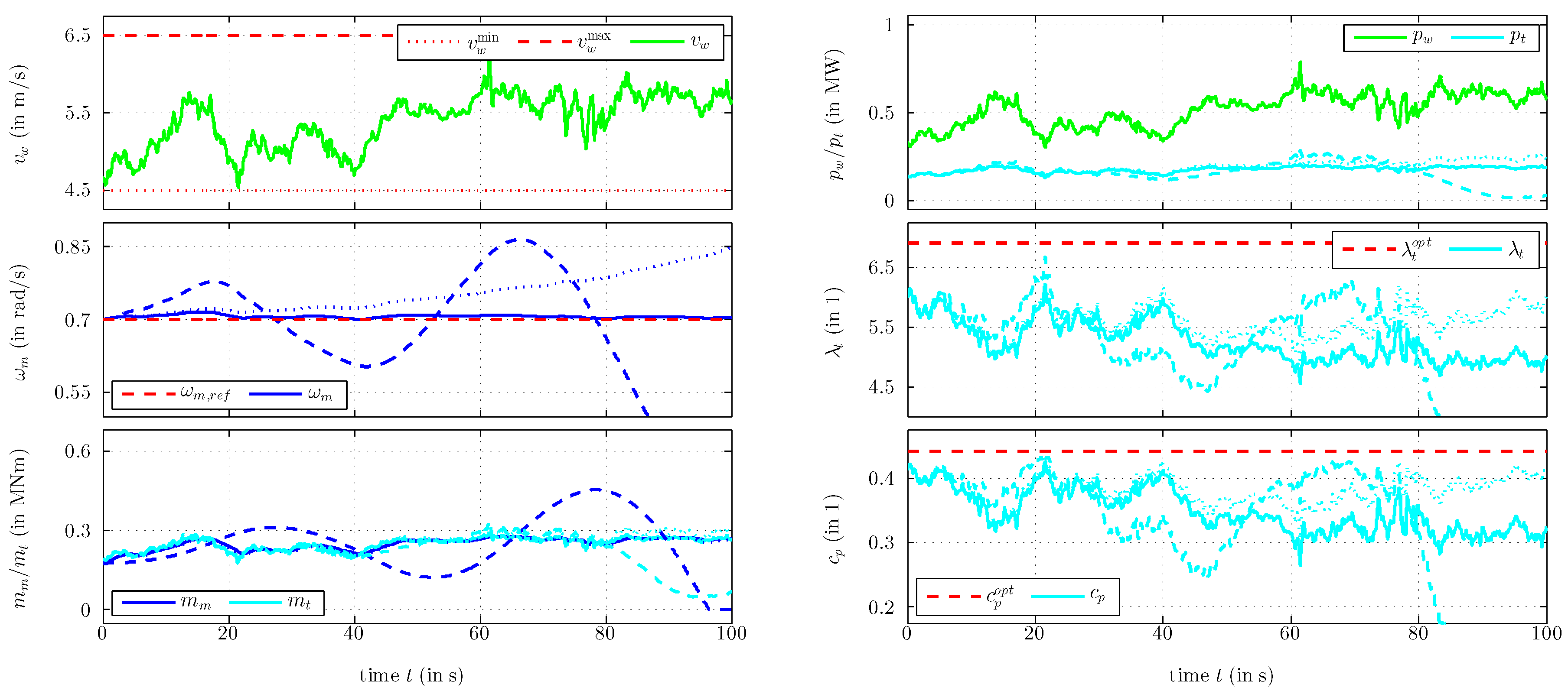
Figure 8.
Simulation results for Scenario 4—reference tracking control performance in regime II.5 for three different controller tunings (a) — stable but slow tuning with and , (b) - - - unstable tuning with and , (c) ⋯ unstable tuning with and : Wind speed , machine speed , machine and turbine torque, wind and turbine power, tip speed ratio and power factor .


Table 1.
System, implementation and controller data.
| Description | Symbols & Values with Unit |
|---|---|
| Matlab/Simulink | solver (fixed step): ode4, sampling time for model |
| sampling time for (discretized) controller implementation | |
| WTS parameter | , , , , , |
| Power factor | , , , , , , |
| , | |
| Controller | , , , , , |
| parameter | , ⇒, , |
© 2018 by the authors. Licensee MDPI, Basel, Switzerland. This article is an open access article distributed under the terms and conditions of the Creative Commons Attribution (CC BY) license (http://creativecommons.org/licenses/by/4.0/).
Share and Cite
MDPI and ACS Style
Dirscherl, C.; Hackl, C.M. Local Stability Analysis and Controller Design for Speed-Controlled Wind Turbine Systems in Regime II.5. Energies 2018, 11, 1251. https://doi.org/10.3390/en11051251
AMA Style
Dirscherl C, Hackl CM. Local Stability Analysis and Controller Design for Speed-Controlled Wind Turbine Systems in Regime II.5. Energies. 2018; 11(5):1251. https://doi.org/10.3390/en11051251
Chicago/Turabian StyleDirscherl, Christian, and Christoph M. Hackl. 2018. "Local Stability Analysis and Controller Design for Speed-Controlled Wind Turbine Systems in Regime II.5" Energies 11, no. 5: 1251. https://doi.org/10.3390/en11051251
Note that from the first issue of 2016, this journal uses article numbers instead of page numbers. See further details here.