1. Introduction
Wind turbine technology and condition monitoring techniques [
1] have been continuously evolving and the operational unavailability of a wind turbine is estimated nowadays to be 3% of its lifetime [
2]. The target of 100% technical availability is therefore becoming realistic and this motivates the research about further optimization of the efficiency of wind kinetic energy conversion. The retrofitting of wind turbines improve the power production is therefore becoming a common practice. This kind of interventions has material and labor costs and producible energy is lost during installation. For this reason, it is crucial to inquire if the performance upgrade justifies the cost of the retrofitting. One key point is that the estimate of the guaranteed energy improvement is commonly provided by the wind turbine manufacturer under the hypothesis of ideal operation conditions of the wind turbines. Instead, the real operation conditions of wind turbines are commonly very different from ideal ones, because of wake interactions [
3,
4,
5,
6,
7] and/or terrain effects [
8,
9,
10,
11].
Wind turbines are subjected to non-stationary conditions because of the stochastic nature of the resource and therefore it makes little sense to compare the energy production of a wind turbine before and after an upgrade. Therefore, commonly, the power curve is studied [
12], which is the relationship between wind speed and power output, and the International Electrotechnical Commission (IEC) [
13] has established widely accepted standards for analyzing it. Basically, the power output of the wind turbine is averaged on wind speed intervals (commonly 0.5 m/s); the dependency on environmental factors is addressed by normalizing the wind speed to standard air density conditions. Further, data describing the wind turbine operating under the wake of a nearby one are filtered away.
The study of the IEC power curve might not be precise enough to distinguish performance improvements of the percent of Annual Energy Production (AEP). Furthermore, as happens in one of the test cases of the present work, it might happen that the approach cannot be employed at all. Other kinds of precision modeling of wind turbines power curve in principle might be employed for studying wind turbine upgrades. This is in general a very fertile field in the scientific literature [
14,
15,
16,
17]. As regards these approaches, the main drawback for their application to the study of wind turbine upgrades is that they are not versatile enough to be applied to the range of different criticality that the study of wind turbine upgrades poses.
Techniques specifically devoted to the study of wind turbine upgrades are needed and this is the main motivation of the present study. This work was a collaboration between academia and industry. The industry is Renvico srl (
www.renvicoenergy.com), owning and managing 335 MW of full-scale wind turbines in Italy and France. Some wind turbines owned by Renvico have been retrofitted in several ways. This study was a pilot test and the decision of extending the retrofitting to the other wind turbines in the corresponding wind farms was based on the assessment, coming from this study, of the real profit on the pilot test cases. The Supervisory Control And Data Acquisition (SCADA) data from the retrofitted and non-retrofitted wind turbines from the wind farms of interest were therefore shared with the University of Perugia. This academia–industry collaboration, as is shown in the following sections, produced methods for the study of power curve upgrades, standing at the frontier of the scientific debate as well as being integrable in the everyday industrial management of wind turbines. This kind of studies on this subject, based on operational data, has very recently been developing in the scientific literature. In [
18], a kernel plus method is adopted for computing wind turbine performance upgrades. In general, kernel regression is a non-parametric method: the available measurements are employed for simulating an output after being weighted with a kernel function (typically Gaussian). In [
18], a modified version of the kernel is proposed (hence, named kernel plus) for addressing dataset dimensionality and bias issues: it has a hybrid structure that includes multiplicative kernel functions in an additive model. This method is employed for studying pitch angle control optimization and aerodynamic retrofitting (vortex generators installation on the blades [
19]). As regards vortex generators, the numerical study of their effect has attracted a certain attention in the scientific literature. In [
20], three different blades equipped with vortex generators have been designed and several stall and pitch regulated wind turbine models have been simulated by means of Blade Element Momentum (BEM) theory. In [
21], the physics of vortex generators on wind turbine DU97-W-300 airfoil is studied through three-dimensional numerical models. In [
22], the S809 airfoil is analyzed. In [
23], the effects of two types of flow control devices, vortex generators and Gurney flaps, on the power output performance of a 5 MW wind turbine, is studied by means of BEM theory. As regards vortex generators and the ex-post study of power production increase through operational data, in [
24], an academia–industry joint study is presented and production of two onshore test case wind farms is considered. On the one hand, SCADA data with 10 min sampling time are employed and, on the other hand, high-frequency power data are employed. The estimates of production improvement are shown to be similar.
Summarizing, in this work, three test-cases are presented and discussed:
Optimization of the pitch angle control system near the cut-in, for an improved start-up;
Blade retrofitting through the installation of vortex generators and passive flow control devices; and
Extension of the power curve for very high wind speed, by raising the cut-out and high wind speed cut-in.
Cases 1 and 2 were studied using the same kind of method: the estimate of the energy improvement is basically computed by comparing the actual production in a post-upgrade period against the simulation of how much the wind turbine would have produced under the same wind conditions if the retrofitting had not been installed. To do this, a model of the pre-upgrade behavior is needed. This was achieved by modeling the pre-upgrade power output of the retrofitted wind turbines by means of an Artificial Neural Network (ANN). The main difference between Case 1 and Case 2 is the selection of the inputs to the model. In particular, Case 2 is challenging because, after the upgrade, the nacelle wind speed measurements are not reliable and therefore cannot be used as inputs to the model. Further, the site is very complex [
10,
25] and it is difficult, albeit necessary, to use nearby wind turbines as references for the environmental conditions. Despite the different complexity, the criticality of Cases 1 and 2 is the same: modeling as precisely as possible the pre-upgrade power output of the upgraded wind turbines.
As regards Case 3 and in general the comprehension of the power curve for very high wind, the criticality is not in the precision of the power curve modeling, because at rated power the errors have a lower relative importance. In this case, the issue is understanding the wind conditions and the logic of the control system before and after the upgrade. This subject has deserved a certain attention in the scientific literature; for example, in [
26], the impact of the hysteresis phenomenon on the energy production is studied. The hysteresis is a control system logic for preventing the wind turbine from beubg subjected to severe dynamic loads: the wind turbine cuts out at a wind speed of the order of 25 m/s and cuts in again when the wind speed lowers several m/s, for example at 20 m/s. This latter wind intensity is known as high wind speed cut-in, to distinguish it with respect to the cut-in, i.e., the minimum wind speed at which the wind turbine operates, which is of the order of 4 m/s. In [
27], control strategies to allow wind turbines to operate above the cut out are studied, based on the study of the fatigue loads. In [
28], an extension of the power curve for very high wind, similar to the one analyzed in this work, is discussed.
On the grounds of the above discussion anticipating some main issues analyzed in this work, it is evident that SCADA-based approaches for the study of wind turbine power curve upgrades must conjugate precision with adaptability to different types of criticality and to different availability and quality of the data. The test cases presented in this work represent an interesting scenario of possible problems and solutions and are therefore useful for the scientific community and industry as well. Summarizing, the structure of the manuscript is as follows. In
Section 2, the test case of pitch angle optimization near the cut in is described.
Section 3 is devoted to the test case of aerodynamic wind turbine blade retrofitting through vortex generators and passive flow control devices.
Section 4 is devoted to the test case of extension of wind turbine power curve above the cut-out. The wind farms, the data sets, the methods and the results are described in
Section 2,
Section 3 and
Section 4 for each test case, respectively. Finally, in
Section 5, conclusions are drawn and further directions of the present work are indicated.
2. Case 1: Improved Start-Up Through Pitch Angle Optimization
2.1. The Wind Farm and the Data Sets
Five three-bladed upwind horizontal-axis wind turbines having 2.5 MW of rated power each are installed in a gentle terrain in France. The rotor diameter with blades is 90 m and the hub height is 80 m. The cut-in is 3 m/s and the cut-out is 25 m/s. The rotor rotational speed goes from 10.3 to 18.1 revolutions per minute (rpm) and at rated power it is 16.1 rpm. The gearbox is three-stage, the generator is double fed asynchronous and the main brake is aerodynamic through pitch angle adjustment.
Three wind turbines (T1, T2, and T3) have been retrofitted with a control system upgrade improving the pitch position for low wind speed, near the cut-in. Two wind turbines (T4 and T5) have not been retrofitted.
The data are collected by the control system with 10 min sampling time and transmitted via an ISDN connection. The SCADA data sets are:
describes the wind turbines operating before the upgrade and goes from 1 May 2016 to 1 September 2017.
describes T1, T2 and T3 operating after the upgrade and T4 and T5 operating without upgrade and goes from 27 September 2017 (date of installation of the improved start-up system) to 18 January 2018.
2.2. The Method
Since the retrofitting affects power output production near the cut-in, data were filtered accordingly between 3 and 7 m/s. The wind speed is measured by the nacelle anemometer and the undisturbed wind speed is reconstructed by the control system through the nacelle transfer function. A subtle point regards how to filter out data characterized by wind turbine malfunctioning: since the regime of interest is near the cut-in, a counter indicating if the wind turbine is ok (producing if there is enough wind, potentially producing if there is not enough wind) was considered the most adequate information for data filtering. For each wind turbine, data are kept when the turbine was okay for 600 s out of 600.
The selected model is a feedforward ANN, with this structure:
The output is the power produced by each wind turbine.
The inputs are nacelle wind speed and wind direction (in the form of sin and cos of the nacelle wind direction ). Therefore, , , .
The wind speed was renormalized according to the meteorological conditions to account for effects due to the variation of the density of the air. The air density averaged on 10 min basis is:
where
B is the measured air pressure,
T is the measured absolute air temperature, and
. For a wind turbine with active power control, the normalization is applied to the wind speed, as follows [
13]:
where
kg/
is the air density in standard conditions (at sea level and 15
C).
The proposed method is as follows: a feedforward ANN architecture was selected and the number of neurons was selected through the
k-fold cross-validation [
29] technique. The data set
was divided
J times randomly in (100-
k)% of the data for training the model and
k% for validating.
k was selected to be 10 for this study, because the objective was validating the model for very short folds to test its robustness.
J was selected to be 300. For each value of the number of neurons, one has
J measurement data sets and
J corresponding simulated data and the mean absolute error
for
can be computed. Averaging over
j obtained an estimate of the average absolute error for a given number of neurons. With this procedure, five neurons were selected.
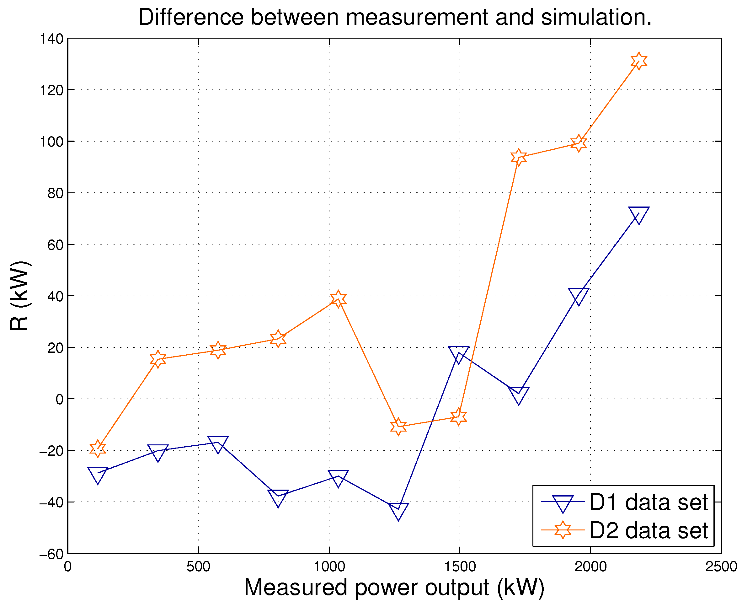
Subsequently, the selected model was employed as follows for estimating the energy improvement: is divided randomly in D0 (75% of ) and D1 (25% of ). For nomenclature consistency, is equivalently named D2. The model was trained with the D0 data set and was employed to simulate the power output using the D1 and D2 data sets. The residuals R between simulations () and measurements (y) were analyzed before and after the installation of the improved start-up. In other words, one has to observe how the residuals change when the improved start-up has been installed.
For
, one computes
Since
is constructed with the relative discrepancies of power data each having the same sampling time (10 min), the quantity
also provides a percentage estimate of the energy improvement. Further, a Student’s
t-test can be performed to detect the difference in the residuals
and
. The
t statistic is computed as
In Equation (
4),
and
are the number of measurements, respectively, in D1 and D2.
and
are the average residuals between measurement and model, respectively, in D1 and D2 and
is given by
where
and
are the standard deviations of the residuals in data sets D1 and D2.
Notice that the model can be run several times, with several different random choices of D0 and D1. This allows having an average estimate of the energy improvement, as well as a standard deviation providing reasonable upper and lower limits.
In this case, it is also possible to study straightforwardly the wind turbine power curve for obtaining a mostly qualitative picture of the performance improvement. This was done and a refinement with respect to the IEC guidelines was adopted: the considerable data population for wind speed between 3 and 7 m/s (else, the adoption of the improved start-up would not justify the installation cost) allows averaging the power output in wind speed intervals of 0.25 m/s without compromising the statistical significance of the analysis.
2.3. The Results
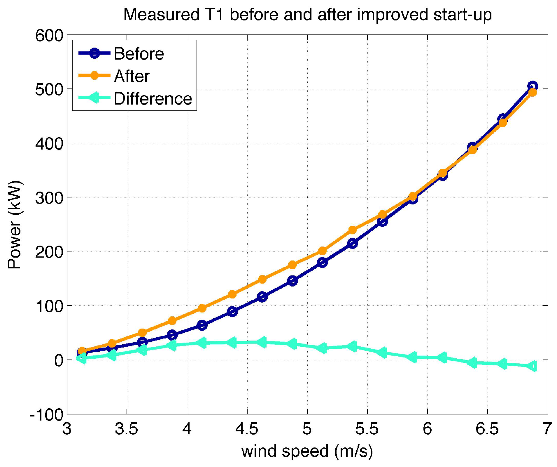
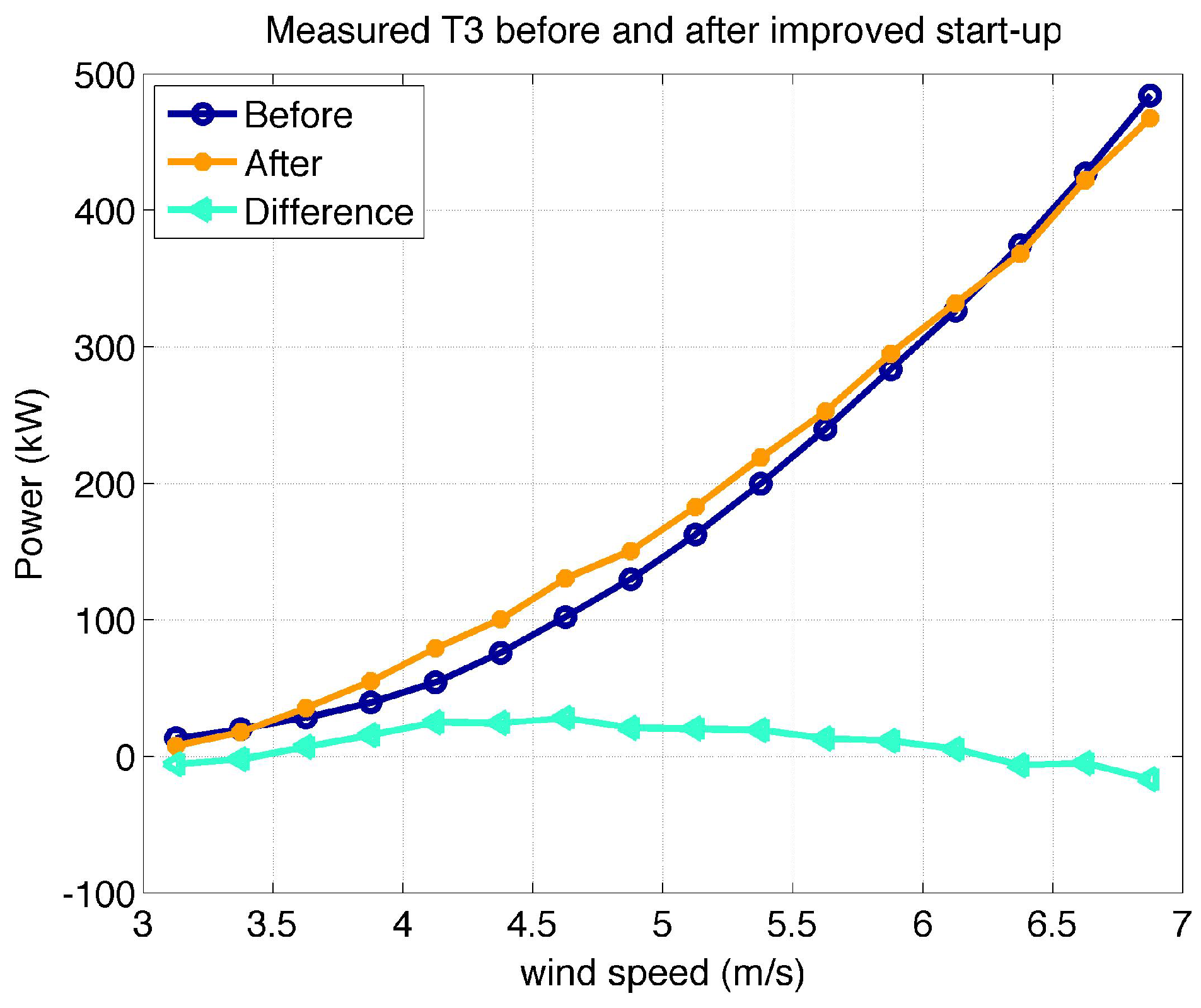
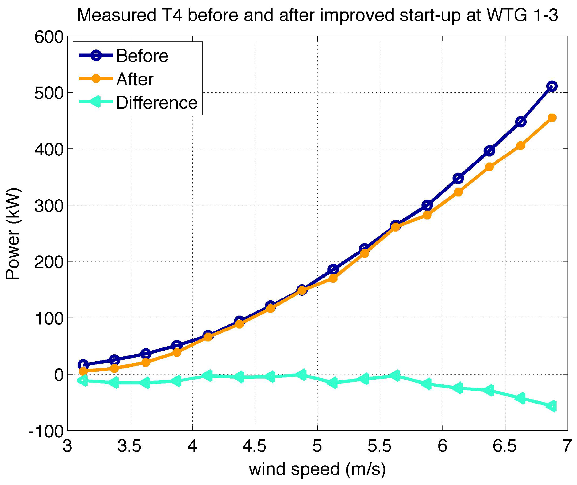
In
Figure 1,
Figure 2 and
Figure 3, it arises clearly that the performances of T1–T3 improved with respect to before the retrofitting and this is especially visible when compared against the power curve of turbine T4 (
Figure 4) measured in the same periods.
For each random selection of D1, the value of the
t statistics (Equation (
4)) is of the order of
for each of the retrofitted wind turbines, which supports quantitatively that D1 and D2 should not be considered data sets coming from the same ensemble. This is a clear indication of the fact that there has been an upgrade.
In
Table 1, the results are reported for the average estimate of the energy improvement for T1, T2, and T3 during the period D2. Notice that this estimate is a percentage referred to the amount of energy produced during D2 from 3 to 7 m/s. Furthermore, notice that in this case the standard deviation of the results can be considered negligible. It is shown below that this does not happen for the test case in
Section 3.
In
Table 2, the values of
in
Table 1 are converted to percentages of improvement with respect to the total energy produced during D2. This quantity is indicated with
.
As a further comment, notice that the above estimate (
Table 2) might not be representative of the long-term wind intensity statistics because it refers to autumn and winter, when there is scarcity of wind near the cut-in with respect to summer. For this reason, the results in
Table 1 have been projected to a twelve-month data set to obtain a simulation of the long-term improvement based on the estimate in
Table 1. The results are collected in
Table 3.
In
Table 3, it arises that the long-term estimate of energy improvement shows significant differences from turbine to turbine: for example, the improvement for T2 is estimated to be twice that for T3. This would not be observable from the power curves in
Figure 2 and
Figure 3 because they are similar. Further, by weighting the power curves against a unique Weibull distribution for the site (as is common in the estimate of Annual Energy Production), the difference from turbine to turbine would not be highlighted. Therefore, the lesson is that being driven by data in the training of the model and in its application is fundamental to observe the energy improvement with a fine grain.
4. Case 3: The Extension of the Wind Turbine Power Curve Above the Cut Out
4.1. The Wind Farm and the Data Sets
The wind farm is the same mentioned in
Section 3. Therefore, please refer to
Section 3 for the information about the wind turbines.
The SCADA data set, here on named D1, employed for the following analysis has 10 min sampling time and goes from 1 January 2017 to 1 January 2018. This data set corresponds to a period during which all the wind turbines of the farm were equipped with the high wind speed control system upgrade.
In
Table 4, the nomenclature for the high wind speed analysis is reported.
Basically, is the average wind speed at which the control system stops the wind turbine; is the high wind speed cut-in, i.e., the average wind speed below which the wind turbine restarts after a cut-out; and is the gust wind speed, i.e., the maximum wind speed at which the control system stops the wind turbine. The SCADA data set at disposal includes minimum, maximum, average and standard deviation of wind speed and power, with 10 min sampling time. Therefore, and were monitored by looking at the average SCADA wind speed, and was monitored by looking at the maximum SCADA wind speed.
4.2. The Methods
The estimation of the improvement in energy production was done through the analysis of SCADA data of wind speed and production. The high wind speed upgrade extends the power curve above the pre-upgrade cut out wind speed; therefore, in this wind speed interval, whatever production measured post-upgrade is gained production because pre-upgrade the wind turbine would be stopped. The downside is that, for wind speed between the post-upgrade cut-in and the pre-upgrade cut-out, the power production is de-rated: according to the pre-upgrade logic, except for the case of wind turbine in hysteresis, the production would be rated power, while, according to the post-upgrade logic, the production is less than rated. Therefore, the energy balance is tricky: if a wind turbine experiences high wind mainly in the unfavorable interval corresponding to de-rating, the upgrade might have a negative effect.
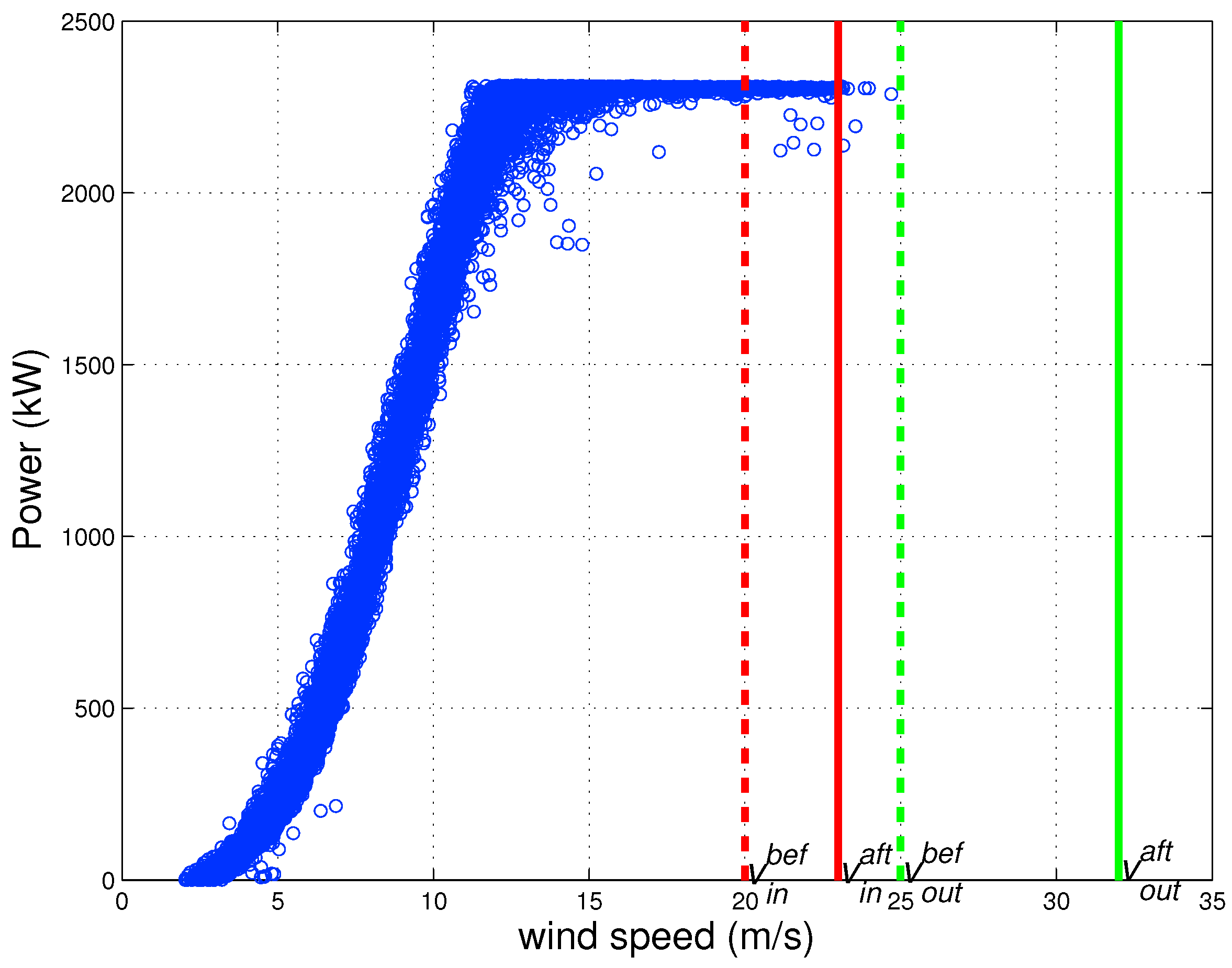
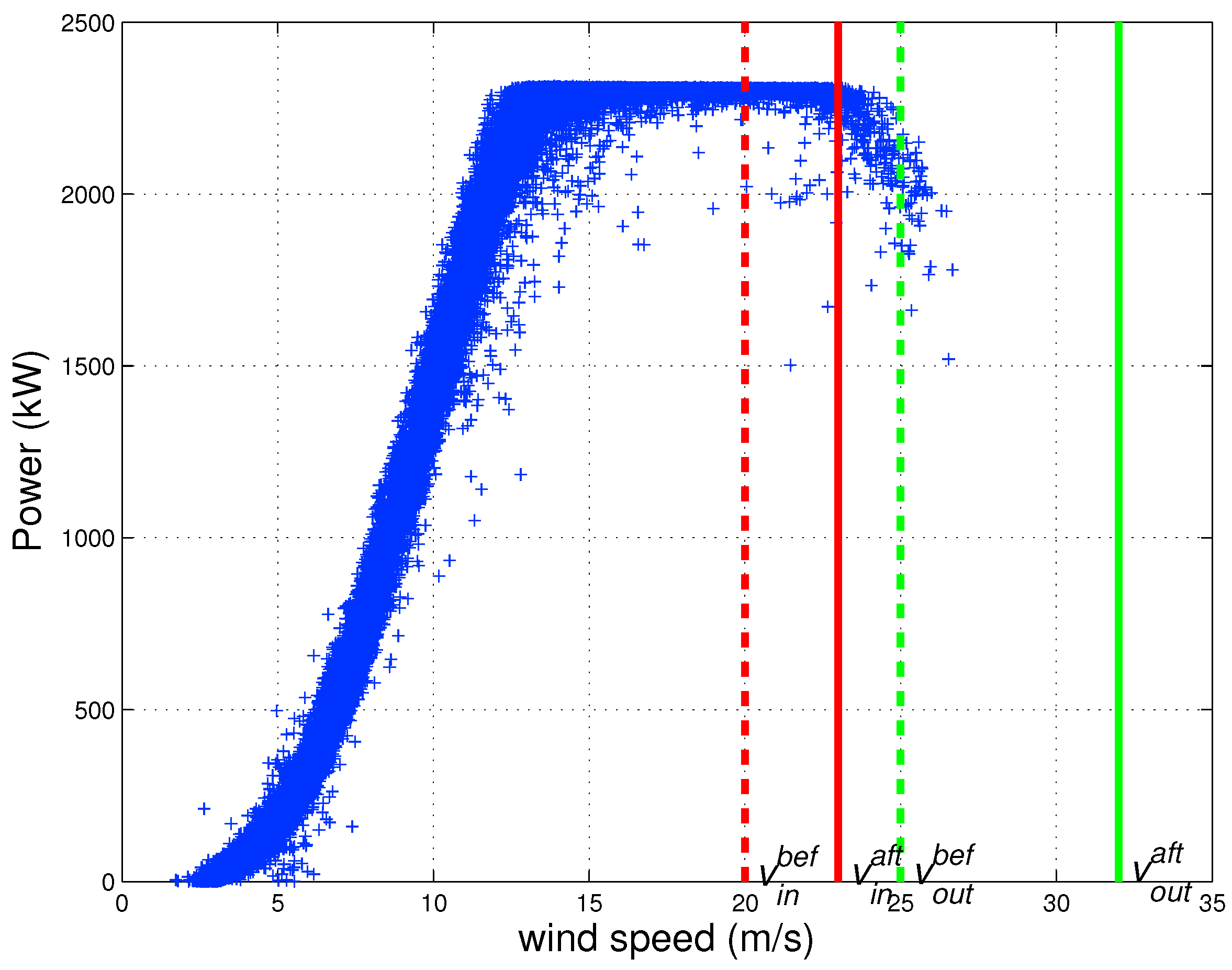
This can be understood by comparing qualitatively the power curves before and after the upgrade. In
Figure 8, a sample power curve before the installation of the upgrade is reported. In
Figure 9, a sample power curve after the installation of the upgrade is reported. In
Figure 8 and
Figure 9, vertical lines are reported in correspondence of
and
(dashed lines) and
and
(solid lines).
To compute the energy balance, the following conditions are therefore verified:
if and : the wind turbine has gained its measured production.
if and : the wind turbine has gained its measured production.
if and and the wind turbine would be in hysteresis according to the pre-upgrade logic: the wind turbine has gained the measured production.
if and and the wind turbine would not be in hysteresis according to the pre-upgrade logic: the wind turbine has lost the difference between the rated and the measured production.
As briefly discussed in
Section 1, the criticality in this case is mainly in the comprehension of the logic of the control system. It is therefore useful to compare the computation of the energy improvement against a simulation of the energy improvement in the same data set. In this case, the power curve for wind speed higher than
is taken from the indications of the wind turbine manufacturer and is here indicated as
P. The following conditions are therefore verified:
if and : the wind turbine should gain rated power.
if and : the wind turbine should gain the power indicated by the P model.
if and : the wind turbine should gain the power indicated by the P model.
if and and the wind turbine would not be in hysteresis according to the pre-upgrade logic: the wind turbine has lost the difference between the rated and the power indicated by the P model.
if and and the wind turbine would be in hysteresis according to the pre-upgrade logic: the wind turbine should gain rated power.
if and and the wind turbine would be in hysteresis according to the pre-upgrade logic: the wind turbine should gain the power indicated by the P model.
4.3. The Results
In
Table 5, the results are reported. The measured energy production improvement (Column 2) and the simulated energy production improvement (Column 3), based on the measured wind conditions, are reported. It is important to notice that the simulated energy improvement is of the order of twice the measured one: 1.06% of the total production of the wind farm against 0.44%.
The mismatch between simulated and measured energy improvement (
Table 5) stimulated a further analysis about its causes. It was observed that the measured power output is very similar to the simulated one according to the indications from the manufacturer, when the wind turbine operates in the high wind region. The point is that the wind turbine is not always operating in the high wind region when it is expected to. An analysis of the wind turbine states during the shutdowns in the high wind speed region has revealed that there are issues related to vibrations and to the control system (spikes in the generator revolutions per minute). Therefore, the lesson is that, if a wind farm owner intends to assess the theoretical profitability of the high wind speed power curve upgrade based solely on the wind conditions measured at wind turbine nacelle, it must be taken into account that, doing this, an upper limit is obtained and the actual improvement can be considerably lower, in a way that is unpredictable without modeling the vibration and the control of the wind turbine, especially in such a complex terrain as in the considered test case.
5. Conclusions
It is non-trivial to estimate the energy production improvement from wind turbines retrofitting. The reason is basically that wind turbines operate under non-stationary conditions, because of the stochastic nature of the wind. Therefore, it makes little sense to compare the energy production before and after an upgrade: the post-upgrade production should rather be compared against a model of the pre-upgrade production under the same conditions.
These issues have become common in the everyday practice of wind turbine management, but their solution needs precision modeling of the power output of the wind turbines and requests flexibility in adapting to the problem and to the quality of the data sets. Therefore, appropriate methods are commonly at disposal of the scientific, rather than industrial, community. On these grounds, this work has been organized as a collaboration between academia and industry and it is hopeful that the outcomes stimulate further cooperation.
The objective of the study was meaningful test cases of wind turbine retrofitting through operational data. They were selected to provide a reasonably comprehensive catalog and the criticality of each case has been discussed such that the outcome of this work is not only in the results, but also in the philosophy and in the methods.
The test cases selected in this work are:
Pitch angle optimization near the cut-in;
Aerodynamic optimization through the installation of vortex generators and passive flow control devices; and
Extension of the power curve in the high wind region through a soft cut-out strategy, based on the raising of the cut-out and high wind speed cut-in.
The first two cases were studied by modeling the power of the retrofitted wind turbines by means of an ANN model. As regards Case 3, the energy improvement was computed by comparing the pre-upgrade to the post-upgrade control system logic according to the measurements of power output and of wind speed at the nacelle of the wind turbines.
Summarizing, the main findings for each test case are the following:
In this case, the data set at disposal made it possible to study the average power curve according to the IEC guidelines and a certain production improvement near the cut-in was observed. The added value of the proposed ANN method is in the fact that, being driven by the wind statistics at each wind turbine, it is possible to distinguish more finely the behavior of each wind turbine. The order of magnitude of the energy improvement is 1% (1.4% in the most profitable wind turbine, and 0.7% in the least profitable one).
In this case, the data set at disposal did not make it possible to study the power curve according to the IEC guidelines because the wind speed measurements at the upgraded wind turbine were unreliable after the installation of the flow control devices. The method was therefore based on the use of the power of a certain number of nearby wind turbines as inputs to model the power of the upgraded wind turbine. The result is that the retrofitting had an impact of the order of 2.0% of the AEP. This estimate is of the order of one third lower than the one provided by the wind turbine manufacturer. Since this wind farm is sited on very harsh terrain, this result supports that complex flow conditions have an impact on the efficiency of passive flow control devices.
The extension of the power curve in the high wind region through a soft cut-out strategy was estimated weighting an order of 0.5% of the AEP of the wind farm since it has been installed. It was observed that this amount is of the order of half the expected, according to the measured wind conditions at the nacelles of the wind turbines. The mismatch between measurement and simulation is explained by the fact that there are frequent shutdowns, due to vibration and control issues, when the wind turbine is expected to work at high wind speed. Since this wind farm is sited on complex terrain, this is more evidence that the production upgrades considerably depend on the conditions at a micro-scale level, especially when rather extreme conditions (wind near the cut-out) come into play.
Further possible directions of the present work include the extension of the test cases and the comparison of several approaches (it would be interesting, for example, to compare with the kernel plus method of [
18]). Moreover, some kinds of retrofitting, as for example Cases 2 and 3 of the present work, call for an improved effort in the condition monitoring of the wind turbines: it would be extremely valuable to model [
31,
32,
33] and to study experimentally how the retrofitting affects the mechanical behavior of the wind turbines, especially for very stressing external conditions as in the case of high wind speed.


