Interaction of Wind Turbine Wakes under Various Atmospheric Conditions


Department of Mechanical Engineering, University of New Mexico, Albuquerque, NM 87131, USA
*
Author to whom correspondence should be addressed.
Energies 2018, 11(6), 1442; https://doi.org/10.3390/en11061442
Submission received: 3 May 2018
/
Revised: 29 May 2018
/
Accepted: 30 May 2018
/
Published: 4 June 2018
(This article belongs to the Collection Wind Turbines)
Abstract
:We present a numerical study of two utility-scale 5-MW turbines separated by seven rotor diameters. The effects of the atmospheric boundary layer flow on the turbine performance were assessed using large-eddy simulations. We found that the surface roughness and the atmospheric stability states had a profound effect on the wake diffusion and the Reynolds stresses. In the upstream turbine case, high surface roughness increased the wind shear, accelerating the decay of the wake deficit and increasing the Reynolds stresses. Similarly, atmospheric instabilities significantly expedited the wake decay and the Reynolds stress increase due to updrafts of the thermal plumes. The turbulence from the upstream boundary layer flow combined with the turbine wake yielded higher Reynolds stresses for the downwind turbine, especially in the streamwise component. For the downstream turbine, diffusion of the wake deficits and the sharp peaks in the Reynolds stresses showed faster decay than the upwind case due to higher levels of turbulence. This provides a physical explanation for how turbine arrays or wind farms can operate more efficiently under unstable atmospheric conditions, as it is based on measurements collected in the field.
1. Introduction
Wind and solar electricity generation exceeded 10% of the total electricity generation in the US for the first time in 2017 [1], with wind accounting for about 8%. Since then, wind-derived electricity has grown by 29.3%, far outpacing the annualized total generation growth of 9.3%. These growth trends for the US energy market are appreciably ahead of the global trends for renewable energy, despite the latter being one of the two fastest growing energy sources globally [2]. Accordingly, there is a considerable recent interest in realistic modeling of wind turbines and wind farms [3,4,5], considering such factors as specific location, relative turbine placement, local weather conditions, and wake interactions.
Two important issues that remain in need of elucidation are the interaction between the atmospheric boundary layer (ABL) and wind turbines, and their wake influence on the downwind turbines. Accurate predictive methods are crucial for turbine-siting, optimizing power output, and reducing fatigue loads. The latter subject is of high practical importance as turbulence leads to repetitive stresses on the turbines that can lead to failure, and the cost of replacing prematurely failed components can become prohibitive, especially for off-shore systems. Several key studies have been conducted on the turbulent wakes from individual wind turbines [6,7,8] and recent efforts have been focused on arrays of turbines. In particular, large-eddy simulations using actuator disks (AD) [9] by Jimenez et al. [10] have shown good agreement with field data obtained by Cleijne [11]. A similar approach with an actuator line (AL) approach [12] coupled to large-eddy simulation (LES) by Troldborg et al. [13] was studied to investigate the wake interaction between two turbines. It was found that the ambient turbulence has a significant impact on the wake development and the subsequent influence on the downstream turbine. They observed improvements in the symmetry of the average blade loadings on the downstream turbine by increasing ambient turbulence level. Similar findings from wind tunnel experiments by Chamorro and Porte-Agel [14] have shown that the wake diffusions were enhanced by increased levels of turbulence from the surface roughness. Their results are consistent with a subsequent LES study using an improved method for actuator disks that accounts for rotation [15]. The upstream turbulence enhances the breakup of the helical wake structure which reduces the velocity deficit along downstream positions. It was found that the wind direction and the turbine positions have a strong influence on the reduction of power generation and increased loadings on the critical turbine components. Using the rotating AD, they conducted further studies with aligned and staggered turbine positions and found the staggered case yielded higher aerodynamic roughness [16]. However, these previous studies were conducted with idealized flow conditions (e.g., neutrally stable ABL) akin to a canonical wall bounded turbulent flow. Several studies on the impact of complex terrain have been reported. Astolfi et al. [17] compared supervisory control and data acquisition (SCADA) data with a Reynolds Averaged Navier-Stokes (RANS) numerical study for a wind farm consisting of four turbines deployed in a complex terrain. Using RANS, it was found that the complexity in the terrain topology altered the local wind and thereby distorted the turbine wake by increasing asymmetricity to the wake profile which ultimately contributed to the wake recovery. Their SCADA analysis gave consistent results. In a study by Subramanian et al. [18], the impact of flat and complex terrain on the turbine wake dynamics was reported using drone-based measurement. They found that the near-wake region was reduced by 35% in complex terrain compared to that of flat terrain. In addition, the degree of anisotropy significantly decreased downstream of the turbine while the measured frictional velocity was consistently higher compared with the flat terrain case. A single wind turbine wake was analyzed by Hansen et al. [19] using SCADA information and a strong correlation was found between the wake movement and the vertical component of the wind which typically reverses its direction during day and nighttime. However, depending on the level of complexity in the terrain’s topology, the flow recirculation can dominate the wake trajectory. Another recent study by Berg et al. [20] performed a LES study on turbine wakes in a complex terrain environment and investigated its impact on the wake positions due to the presence of a strong recirculation zone. A similar study by Castellani et al. [21] investigated the impact of complex terrain on the wind farm performance. They also studied the atmospheric stability factor in the performance of wind farms. The atmospheric stability effect on turbulence intensity and turbine power loss was studied by Hansen et al. [22], in which it was found that the maximum power deficit and the turbulence intensity had a linear relationship. A stable atmospheric condition was found to yield the largest power deficits as the turbulence intensity was low compared to the other stability classes.
In the present study, the atmospheric variability was investigated for a two multi-megawatt wind turbine case using LES. In particular, the aero-elastic response of the turbine blades was included by coupling the actuator lines with FAST (Fatigue, Aerodynamics, Structures, and Turbulence) code [23]. Neutral and unstable ABLs with various surface roughness, representing land-based and offshore conditions [24], were studied to characterize the turbine wakes, the turbulence production generated by both upstream and downstream turbines. Furthermore, power production changes due to various atmospheric conditions were discussed.
2. Methodology
2.1. LES Framework
Atmospheric boundary layers with various aerodynamic surface roughness and stability conditions were studied using large-eddy simulation. An incompressible formulation of the continuity equation (Equation (1)) and the momentum equation (Equation (2)) (which includes the Coriolis force, the buoyancy force, and the aerodynamic force at the actuator point), and the potential temperature transport equations (Equation (3)) are shown in the following:
The tilde on the velocity vector denotes the spatially resolved component. The modified pressure is defined as where . The filtered static pressure term is and ρ0 is the constant density. The mean pressure term is whose spatial gradient acts to drive the flow convection. The last term, , represents the hydrostatic pressure. The deviatoric part of the fluid stress tensor is where is the Kronecker delta. The subgrid-scale (SGS) stresses are included in the τij term. The SGS flux was computed using the Smagorinsky [25] model with the Smagorinsky constant of 0.13. Using the local cell dimensions, , and , the filter length scale was based on . The latitude () of 45° and the planetary rotation rate ( of 7.27 × 10⁻⁵ rad/s served as inputs to the Coriolis force defined as f = 2[0, cos(), sin()]. The buoyancy effect was calculated using the Boussinesq approximation, where g is the gravity, is the resolved potential temperature, is the reference temperature taken to be 300 K. The aerodynamic force computed by the actuator line method is denoted as Fi. The temperature flux, qj, used in the transport equation for the resolved potential temperature equation (Equation (3)) is defined as below:
The SGS viscosity and the turbulent Prandtl number (based on Moeng’s [26] approach) are and , respectively. The governing equations were solved using the Simulator for Offshore Wind Farm Application (SOWFA) [27] which employs the second-order central differencing scheme to discretize the above equations on an unstructured collocated finite-volume formulation. The Rhie and Chow [28] interpolation method was used to avoid checkerboard pressure-velocity decoupling. The Pressure Implicit Splitting Operation (PISO) [29] method with three-step correction was employed for second order temporal accuracy.
2.2. Atmospheric Boundary Layer
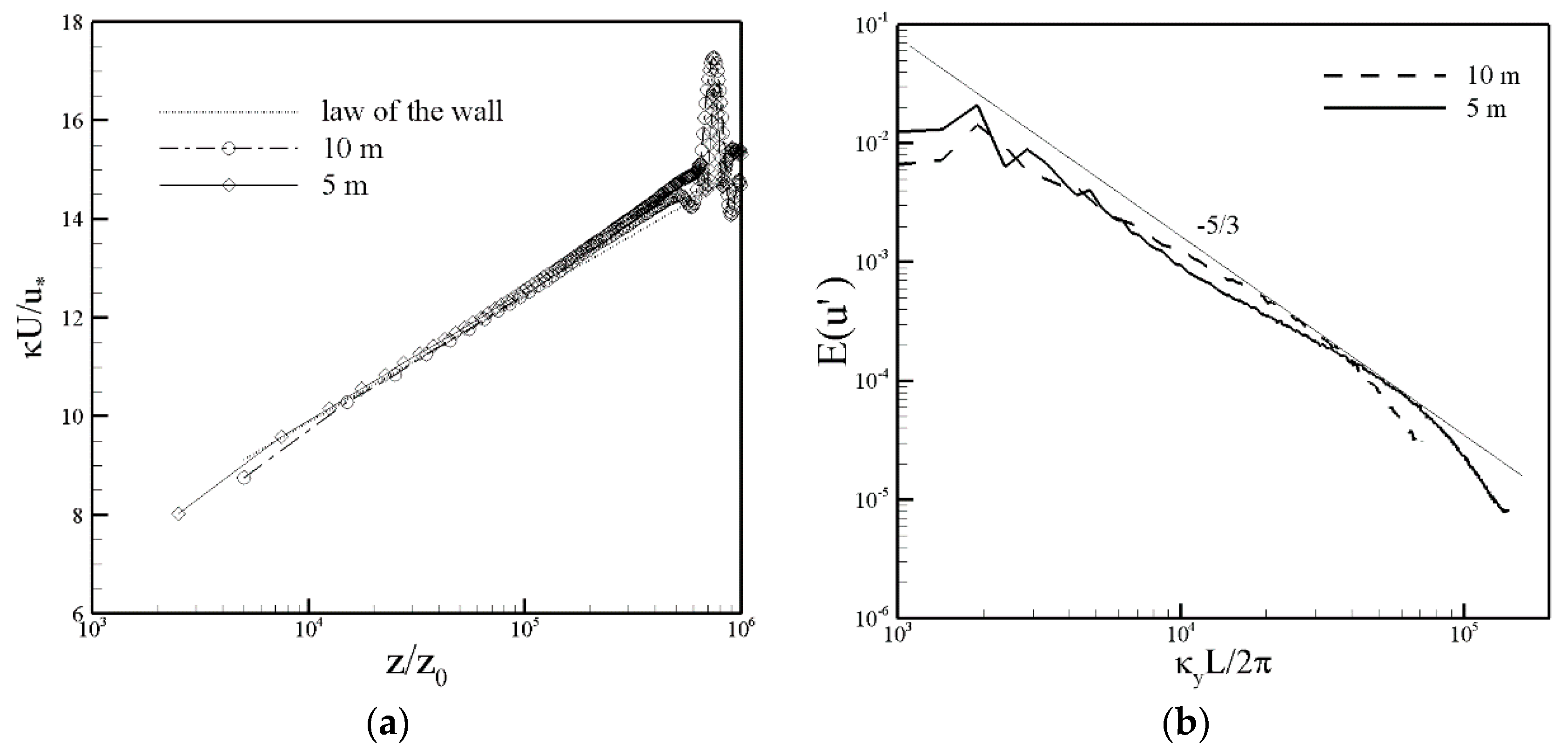
Two atmospheric stabilities and two surface roughness cases were studied in the present investigation (Table 1). Neutrally stable and unstable ABLs were the two stability classes in which an adiabatic condition was used for the neutral case, while an average surface temperature flux was set to be 0.04 K·m/s for the unstable case. Neutral atmospheric conditions refer to zero temperature gradient within the boundary layer due to lack of heat flux exchange at the ground by the sun. This condition occurs from dawn to early morning times. Unstable atmospheric conditions occur when the sunlight radiates the ground and raises the local air temperature, which causes the vertical rise of air parcels. This phenomenon is typical during daylight times. Low and high surface roughness were investigated with the two stability cases, where the roughness height was set at 0.001 m and 0.2 m, which are representative of offshore and land-based conditions [24], respectively. The potential temperature profile starts at 300 K with a capping inversion occurring from 700 m to 800 m which increased the temperature by an additional 8 K. A lower rate in the temperature increase occurred above the capping inversion at a constant rate of 0.003 K/m. The mid-point within the capping inversion, Zi = 750 m, is defined as the boundary layer height. The horizontal average wind speed of 8 m/s was fixed at the hub-height, Z = 90 m. The streamwise mean velocity profiles from the NLABL (Neutrally stable case, Low surface roughness Atmospheric Boundary Layer, Table 1) case with 5 m and 10 m resolutions are shown in Figure 1a. For both resolutions, reasonable agreement with the log-law can be seen. The large peaks at Z/Z0 ~ 7 × 10⁵ were caused by the temperature capping inversion in which the velocity profile inflected towards higher speeds above the boundary layer height. The resolution effects on the boundary layer flow were more pronounced in the velocity spectra as shown in Figure 1b. While the inertial range that matches the −5/3 power law curve was similar in both cases, higher wave lengths were better resolved for the 5 m case before smaller turbulence scales dissipate via the sub-grid scale closure. Therefore, the 5 m grid resolution was chosen for the background mesh as well as the precursor inflow boundary condition. Total computational resources of approximately one million computational hours were required for this study.
2.3. Computational Domain
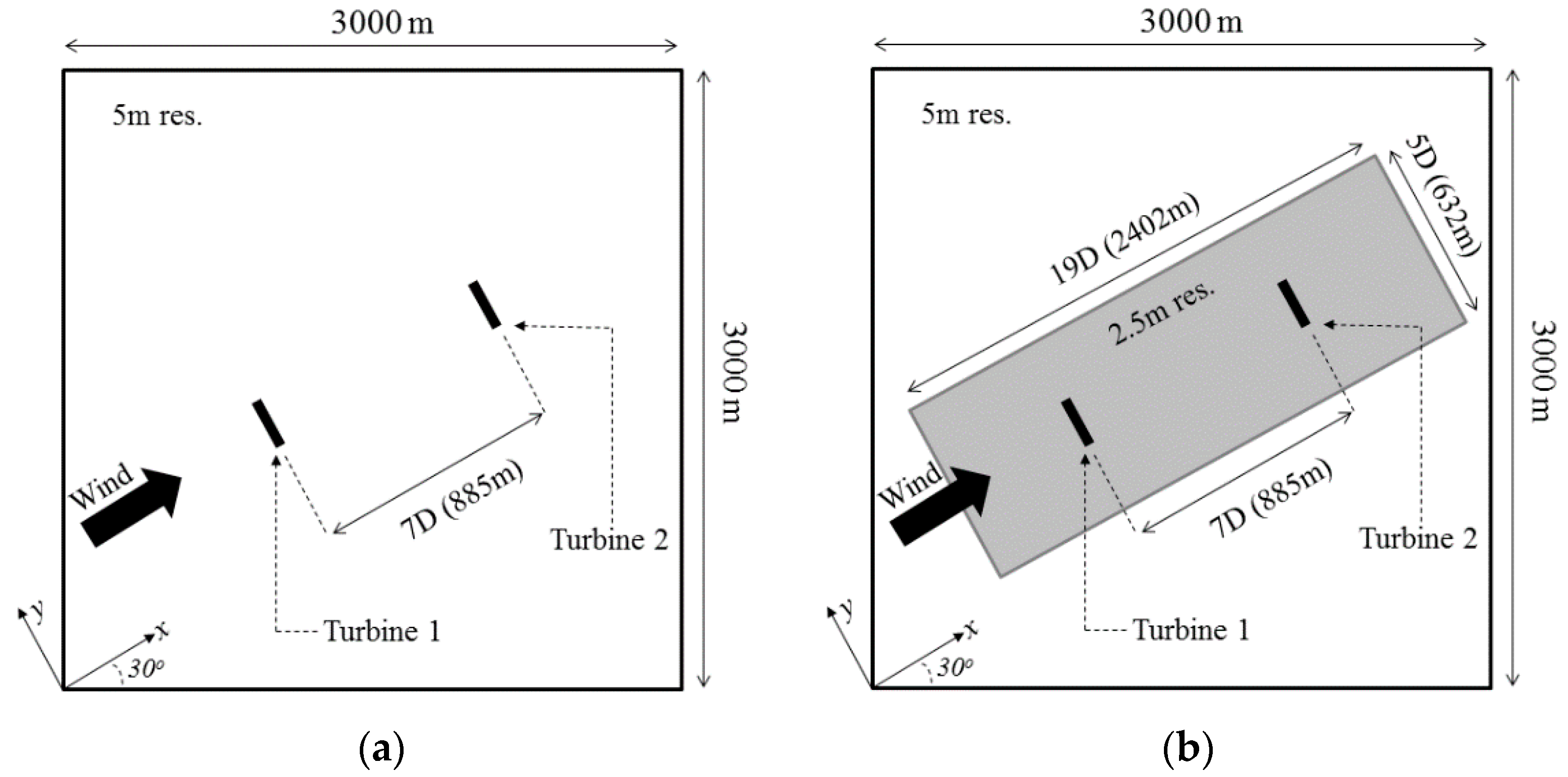
The horizontal dimension of the computational domain in the present study, was 3 km by 3 km with a vertical height of 1 km as shown in Figure 2. The mid-point of the two National Renewable Energy Laboratory (NREL) 5-MW wind turbine positions, which were separated by seven rotor diameters, aligned with the center of the domain. By limiting the present study to two turbines rather than multiple turbines (akin to the interior of a wind farm), a fundamental understanding of the upstream turbine wake impact on that of the downstream velocity deficit recovery, Reynolds stress, power generation can be achieved. The angle of the line connecting the two turbines were rotated 30° counterclockwise to align with the mean wind direction. Two steps were involved in the mesh generation process. Initially, the grid cell size was uniformly 5 m in all three primary axis directions (Figure 2a) which was identical to the precursor domain. While maintaining the 5 m resolution for the background mesh, a rectangular region shown in Figure 2b that includes the two turbines is refined to a 2.5 m cell which yields a total of approximately 92.1 million cells for the entire domain. In this refinement process, the cell sizes are divided evenly in all three directions such that uniform grid spacing is maintained within the refinement zones. The surface stress and the temperature flux conditions are imposed at the surface boundary following Moeng’s approach [26]. The friction velocity is approximated using the Monin-Obhukov similarity theory [30]. The west and the east boundaries were imposed with inflow and the outflow conditions, while a free stress condition was imposed at the top boundary. A periodic condition was used for the north and the south boundaries.
2.4. Wind Turbine Model
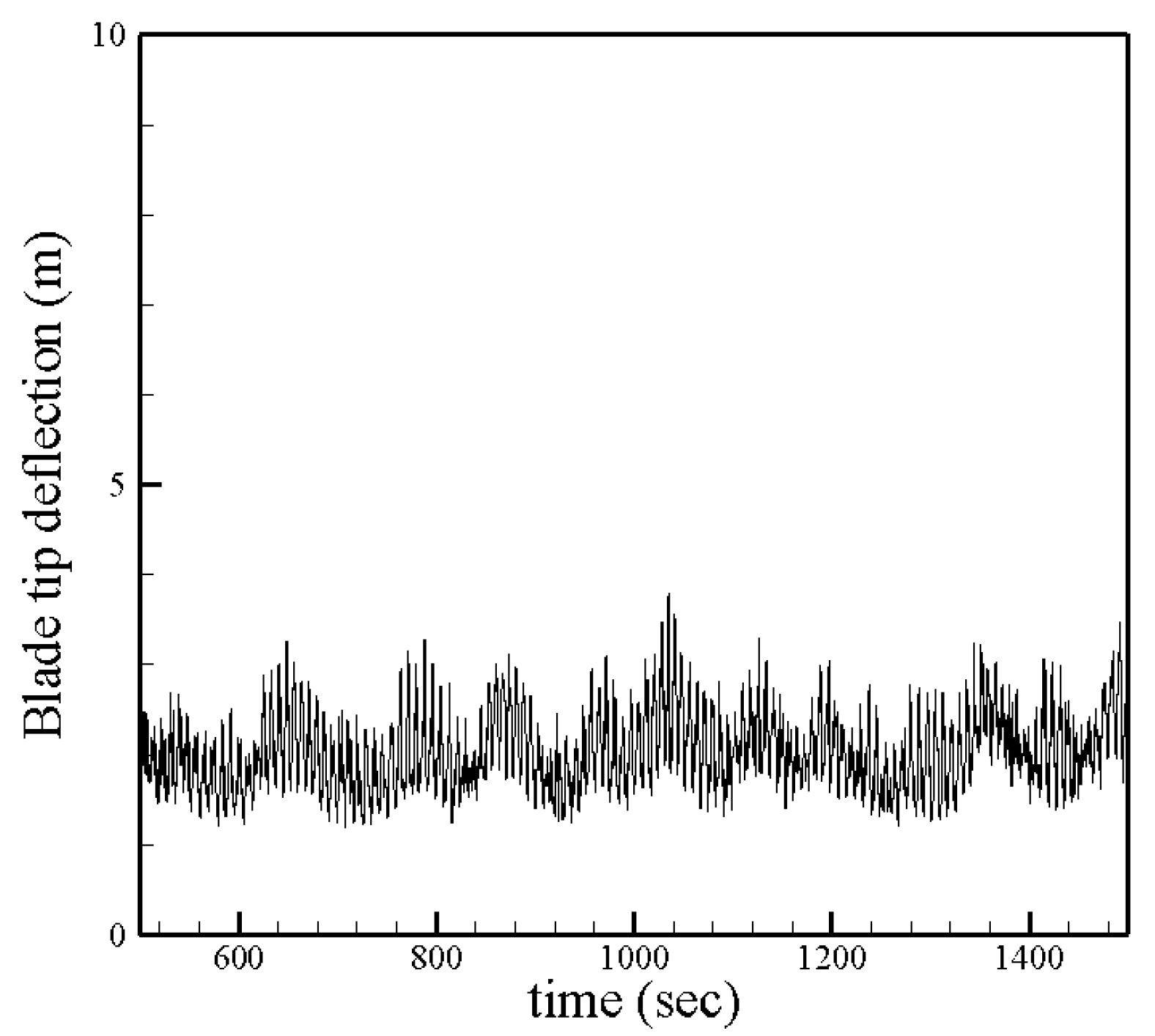
The National Renewable Energy Laboratory (NREL) 5-MW reference turbine model [31] was used in the present study. It is an upwind horizontal-axis turbine with three-blades with a swept diameter of 126 m installed at a hub-height of 90 m. The rated power of 5 MW occurs at a wind speed of 11.4 m/s with a rotor speed of 12.1 revolutions per minute (RPM). At a hub-height-average flow speed of 8 m/s, the turbine rotor spun at approximately 9 RPM generating 2 MW of power. The dynamic response of the NREL 5-MW turbine was computed using FAST which is an aero-elastic simulation tool developed by NREL. The aerodynamic forces from the blades which are represented by Fi in Equation (2) in the atmospheric flow solver, were fully coupled with FAST which employed a combined modal and multi-body dynamics formulation for the flexible blades and the tower, assuming small deflections. A typical blade tip deflection in the present work is shown in Figure 3 where the maximum deflection of 3.5 m was observed, which corresponds to 2.8% of the rotor diameter. This length would only incur, at most, 1.6° deflection angle at the blade root. The time step size was restricted for the blade tip to traverse no more than a grid cell per time-step (Δt = 0.02 s). The actuator line representation consisted of a two-way coupling in which the flow information was used as an input to compute the aerodynamic forces which fed back to the flow with new positions. The peak magnitude of the forces at the actuator points and the projection width was controlled by the Gaussian width [12] which was set as equal to twice the grid cell length. The resolution of 5 m used in the precursor domain (Figure 1b) to generate the turbulent inflow conditions captured a wider inertial range that enabled us to resolve higher wave lengths in comparison to the precursor domain with a 10 m resolution used in a previous study by Churchfield et al. [32]. His work demonstrated that the power predictions for individual turbines, using a similar grid nesting procedure and Gaussian width, yielded good agreement with the field measurements. In the present study, the turbulent kinetic energy (TKE) was measured at various locations downstream of the turbine using a coarse test grid (2, 2 2) and a maximum of 2.3% difference was observed when compared with the TKE results obtained from the original high-resolution grid (Figure 2b). Therefore, no further grid independence study was performed in this investigation.
3. Results
In this section, the dependency of the atmospheric conditions on instantaneous and time-averaged velocity contours, profiles of turbulent kinetic energy (TKE = , where , and are fluctuating velocity components), and Reynolds shear stresses, and the power production are discussed.
3.1. Velocity and Turbulent Kinetic Energy
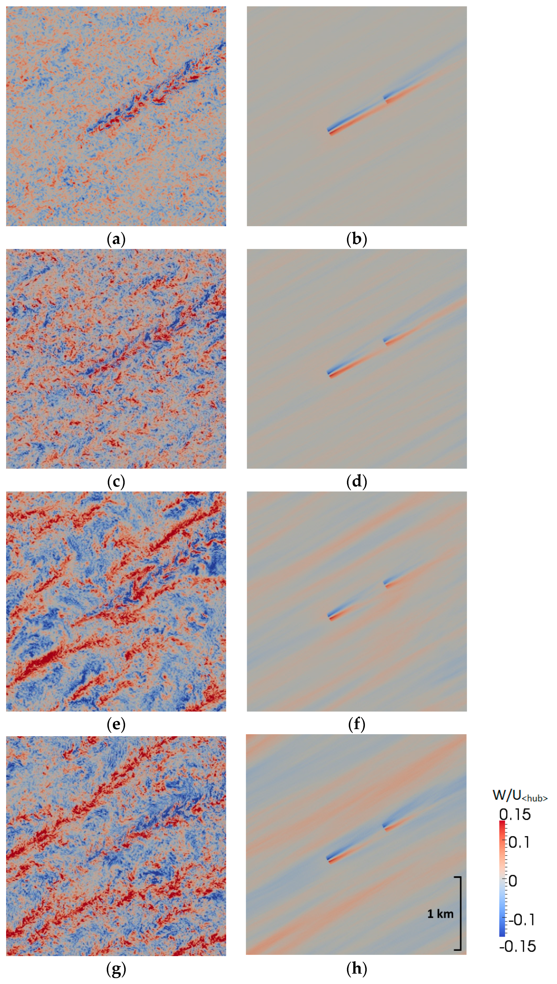
Instantaneous and time-averaged streamwise velocity contours at the hub-height (Z = 90 m) are shown in Figure 4. The wake from the upwind turbine for the NLABL (Figure 4a) case was in line with the general wind direction. The size of the wake structures increased approximately 1D~2D downstream of the turbines as their coherency became unstable. The downstream turbine, being exposed to higher levels of turbulence, yielded large-scale unsteady motions in the wake structures. The time-averaged NLABL, shown in Figure 4b, reveals that the velocity deficit is pronounced in the wake of the downstream turbine due to the upstream wake. As the surface roughness was increased in the NHABL (Figure 4c) case, the coherency was further disturbed such that meandering wake structures can be observed. This enhanced the recovery of the boundary layer flow as the lengths of the wakes were shorter than that of NLABL, as shown in the time-averaged case (Figure 4b,d). The meandering wakes were further exacerbated in the unstable atmosphere cases, ULABL (Figure 4e) and UHABL (Figure 4g), primarily due to the updrafts of the thermal plumes. Hence, the recovery of the wake deficit was expedited relative to the neutral cases as shown by the time-averaged flow fields (Figure 4f,h). The updrafts of the thermal plumes can be seen in Figure 5 which is indicated by the large red streaks extending up on a kilometer scale (Figure 5e,g). Note that the rotating wake structures indicated by the alternating patterns of red and blue wings, shown in the NLABL (Figure 5a) case, were disrupted by the surface roughness (NHABL, Figure 5c) and further disorganized by the updrafts shown in ULABL (Figure 5e) and UHABL (Figure 5g). The lengths of the wakes shown in the time-averaged vertical velocity contours were significantly shorter in the unstable cases than that of the neutral cases due to the enhanced mixing in the boundary layer.
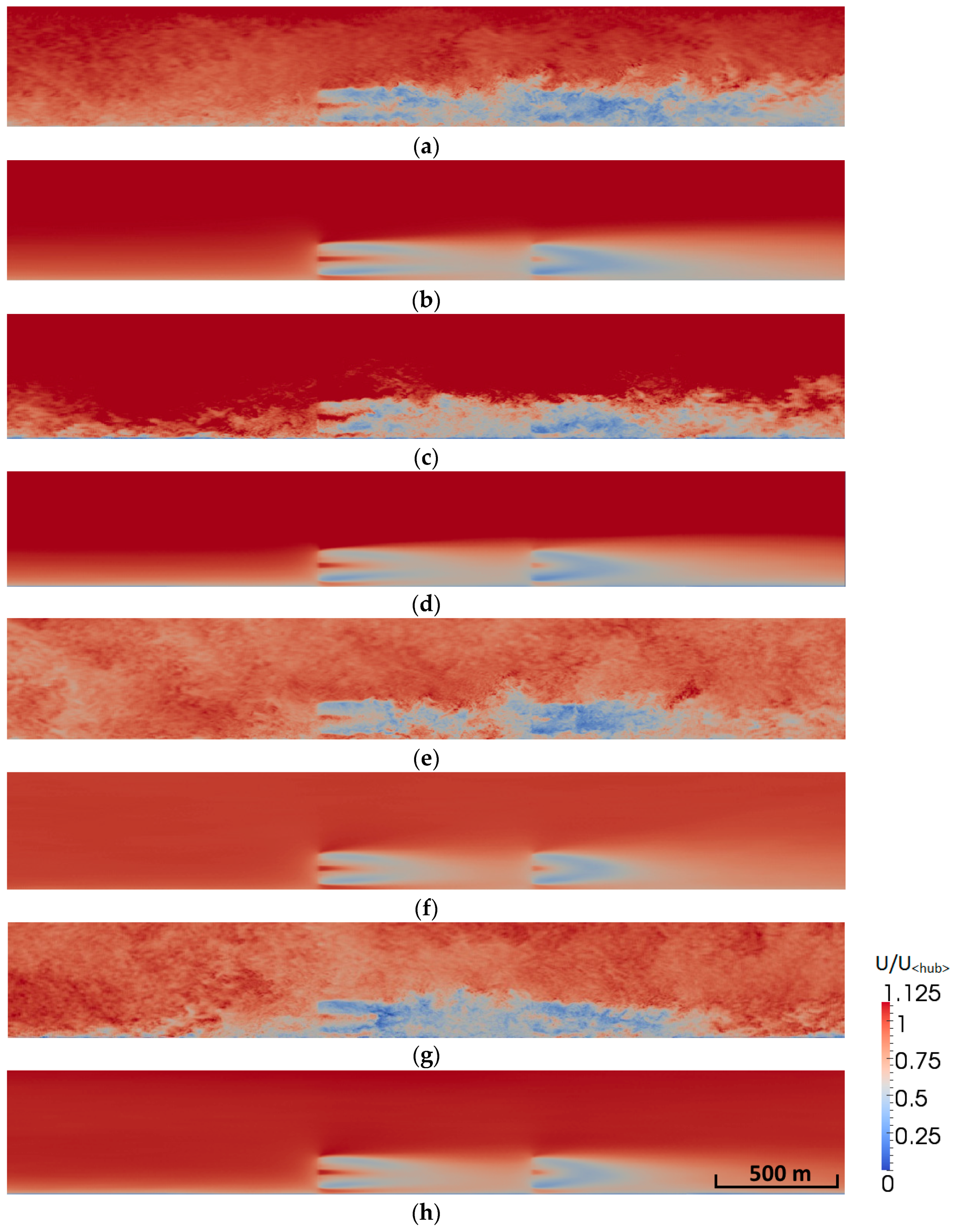
Vertical cuts of the streamwise velocity contours shown in Figure 6 display the evolution of the instantaneous wake structures in further detail. Low momentum fluid near the wall, indicated by the blue regions in Figure 6c (NHABL) and Figure 6g (UHABL), were caused by the increased viscous layer induced by the surface roughness. As shown in the previous figures, the large scale unsteady motion of the turbulent wake can be observed by the second turbine shedding off wake parcels. Furthermore, the increase in the boundary layer height downstream of the turbines can be observed for the neutral cases shown in the time-averaged NLABL (Figure 6b) and NHABL (Figure 6d) cases. Due to the expeditious recovery of the wake boundary layer for ULABL (Figure 6f) and UHABL (Figure 6h), the wakes of the second turbine were approximately as short as that of the upstream, which implied that increased power generation can be expected compared to the neutral cases.
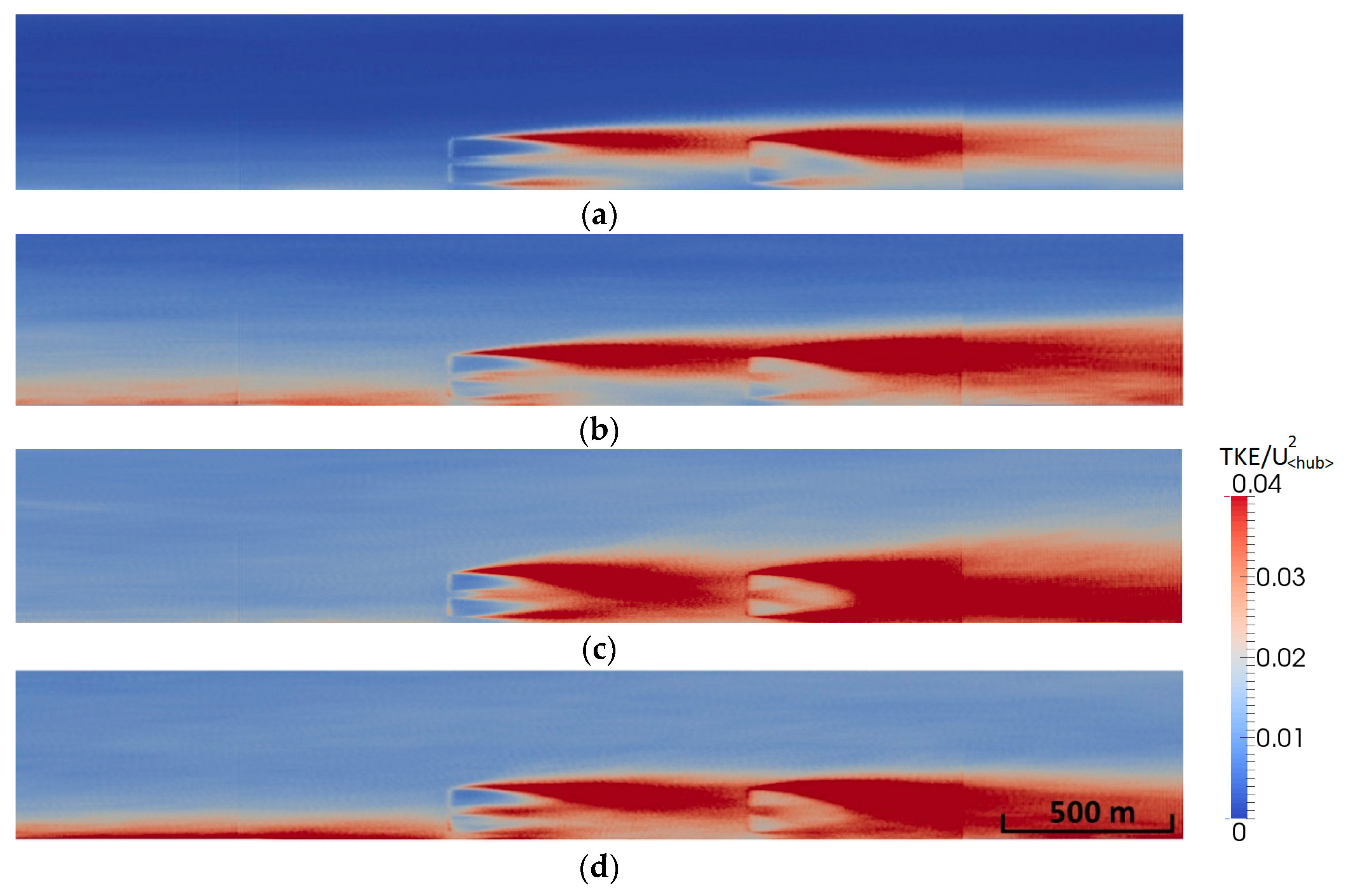
The contours of TKE based on the resolved velocity fluctuations are shown in Figure 7. Note that the effect of the local refinement of the grid, shown in Figure 2b, are reflected in the TKE contours where discontinuous lines can be clearly seen towards the exit of the domain due to the abrupt changes in the grid resolution. Higher levels of TKE are observed near the ground upstream of the first turbines for NHABL (Figure 7b) and UHABL (Figure 7d) due to the increase in the viscous layer. In addition, streaks of intense TKE extending from the blade tip at the top can be seen in all cases where the unstable cases yielded premature decay consistent with the velocity contours shown in Figure 6. Note that the TKE is higher for the top rotor tip as strong shear layers developed from the boundary layer flow interacting with the rotating turbines. The TKE at the top rotor tip was intense and persisted for a long distance downstream in the NHABL (Figure 7b) case. In contrast, the length of the intense TKE were approximately 3D~4D for the unstable cases (Figure 7c,d).
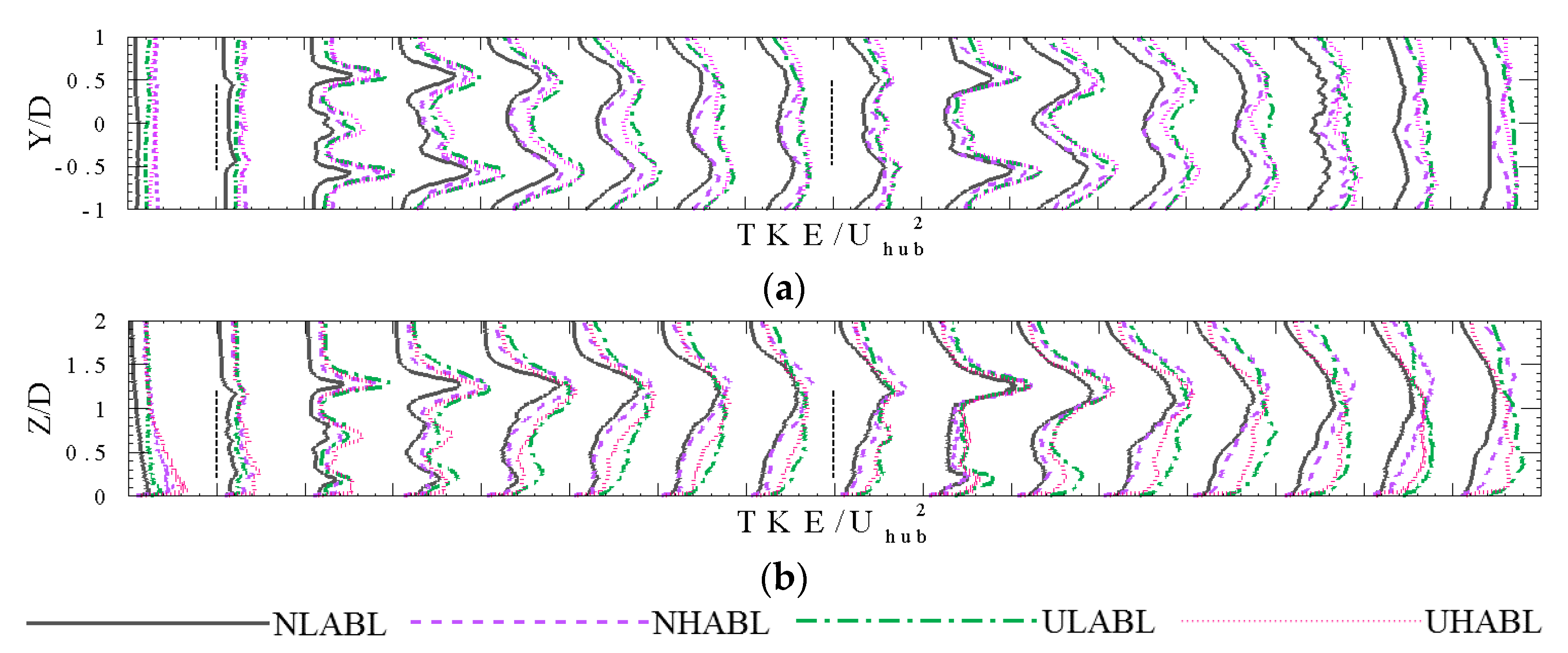
The horizontal profiles of TKE were taken at hub-height (Z = 90), while the vertical profiles were extracted at the line connecting the turbine towers which are shown in Figure 8. The inflow conditions (X = −1D) exhibited higher levels of turbulence with increasing surface roughness and instability of the atmosphere. As the flow traversed the first wind turbine, large peaks of TKE near the blade tips were found approximately 1D downstream of the turbine due to the breakup of the tip vortices, as shown in Figure 8a. The TKE peaks shown in vertical profiles (Figure 8b) were larger in intensity at the blade tip at its maximum height (Z/D = 1.21) for both the upstream and the downstream turbine positions, which was due to the shear layer that forms with the rotational plane and the incoming boundary layer. The TKE peaks were of significant sizes in the unstable ABL cases, but decayed quickly and redistributed their energy to the neighboring regions, thus yielding a flatter profile along the downstream distance. The wake turbulence impinged upon the downstream turbine, yielding even higher TKE peaks, which suggests that the load stresses induced by turbulence can be significant for turbines exposed to upstream wakes.
The turbulence intensity along the blade tip at its top (Z/D = 1.21) is shown in Figure 9 which indicates that the TKE profiles exhibited two cycles of rapid rise followed by gradual decay downstream of the turbines. The second TKE peaks which occurred approximately 1D downstream from the second turbine have higher magnitudes for the NHABL and UHABL cases. The incoming TKEs at X = 6D were consistently larger for the high surface roughness cases and the combination of wake turbulence from the upstream turbines and surface-induced turbulence contributed to the large peaks. The direction of the momentum transport due to turbulence can be seen in the Reynolds shear stress profiles in Figure 10. The correlation between the fluctuating components of u and v (Figure 10a) shows a negative peak at Y/D = 0.5.
The strong shear layer at the wake’s edge pulled the low momentum fluid (u′ < 0) from the wake deficit region to the outer-wake region with positive flux in the y-axis direction (v′ > 0). The high momentum fluid (u′ > 0) from the outer-wake region was transported to the wake deficit region via negative spanwise velocity fluctuation (v′ < 0). The combined effect yielded negative correlation for u′ with v′ at the wake edge position at Y/D = 0.5. Positive correlation occurred at Y/D = −0.5 due to the symmetry in the shear layer in which the sign of the velocity fluctuations was the opposite sign of those at Y/D = 0.5. The peaks shown in the vertical profiles for <u′w′> in Figure 10b were generated based on the same mechanism. However, the magnitudes of the positive peaks near the ground were smaller compared to those at the blade tip at its top (Z/D = 1.21) due to the viscous layer which mitigates the fluctuations. Two rotor diameters downstream of the first turbine exhibited the largest peaks which decay with further distances. Larger peaks and spatial variations were observed downstream of the second turbine due to the added wake turbulence. The remaining component of the Reynolds shear stress, <v′w′>, did not show any pronounced peaks indicating that v′ and w′ were weakly correlated.
3.2. Power Generation
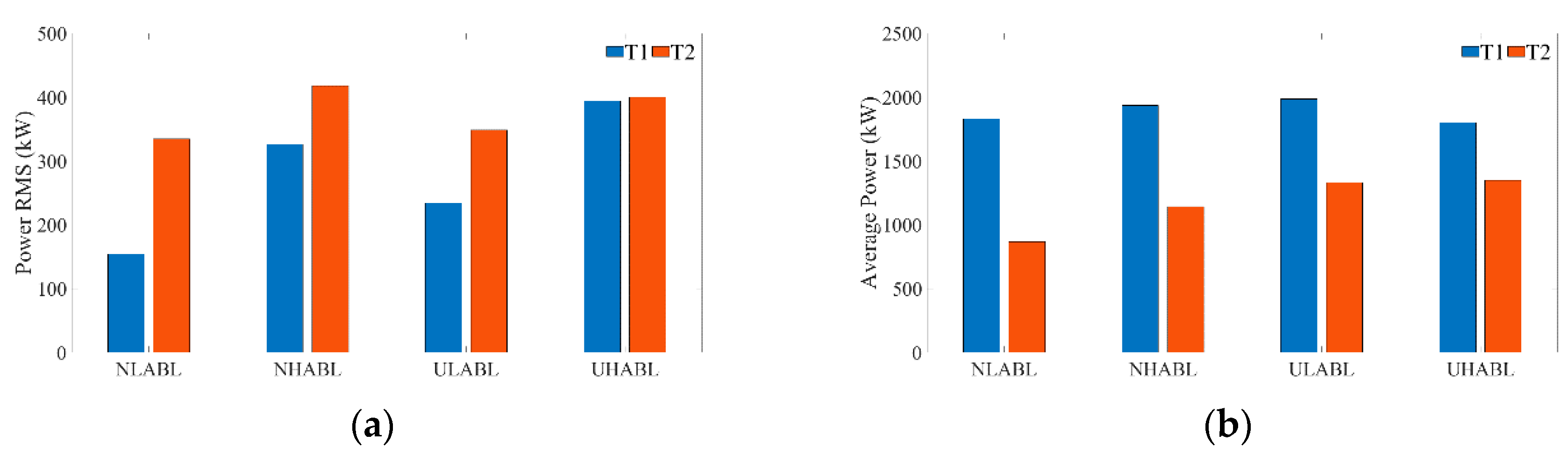
The atmospheric and the wake turbulence affected the power production of the turbines shown by the large fluctuations in the power signal in Figure 11. The increasing trend of the fluctuation magnitude can be observed alongside the surface roughness and the atmospheric instability. In the low roughness cases (NLABL and ULABL), the signal patterns of the downstream turbine power generation roughly followed the upstream turbine power output. Conversely, the signal patterns significantly differed from that of upstream turbines for the high roughness cases (NHABL and UHABL) due to the meandering of the upstream wakes. The undulatory movement of the wake (velocity deficit) trajectory resulted in power increases when the wake meandered away from the downstream turbine. This allowed the high-speed flow to enter the downstream rotor and the torque controller responded with a faster spinning rotor. However, the repeated meandering motion of the wake can also contribute to cyclic loads on essential components of the blades, which can lead to fatigue damage. The power root mean square (RMS), shown in Figure 12a, is largest in the NHABL case for the downstream turbine. As expected, the generator power output is lower from the downwind turbine, especially in the NLABL case where an approximately 60% reduction was seen. However, with the increasing surface roughness and atmospheric instability, the recuperation of the power loss for the downwind turbine was improved, which is consistent with the quickly decaying wake deficits seen in the time-averaged velocity contours (Figure 4, Figure 5 and Figure 6). Field measurements have shown that wind farms generate more electricity in an unstable atmosphere [33,34].
4. Conclusions
Large-eddy simulations of two utility scale 5-MW turbines were performed to assess the effects of four representative atmospheric boundary layer flow cases for typical land and ocean conditions at different operation times. These cases were separated into neutrally stable and unstable groups. Each of these groups were further divided into low and high surface roughness cases. Increases in the surface roughness and atmospheric instabilities contributed to the wake recovery and the increase in the turbulence stresses. For cases involving the unstable atmospheric boundary layers, thermal updrafts from the surface increased the turbulence mixing. This led to an accelerated decay in the velocity deficit. Notable concentrations of turbulent kinetic energy were observed near the blade tip positions due to the breakup of the tip vortices approximately one rotor-diameter downstream of the turbine. The turbulent kinetic energy was observed to increase near the downstream turbine, mostly due to the addition of the upstream wake turbulence. The TKE peaks were of significant sizes in the unstable ABL cases, although these decayed quickly and redistributed their energy to the neighboring regions due to the mixing of ambient turbulence present in the unstable ABL. Similar results were obtained for the decay of Reynolds shear stresses with respect to the instability of the ABL. This expedited wake recovery mechanism was essential to improving the energy capture by the downstream turbines. For the neutrally stable cases, the power generation loss was as high as 53%. In contrast, the unstable and high surface roughness case was characterized by an energy loss of 25% for the downstream turbine. In summary, our study strongly suggests that wind farms can operate more efficiently under unstable atmospheric conditions, which is consistent with field observations. These findings are important both for realistic modeling of wind farms and for determining optimal wind farm locations. Future studies will include the interaction of wind turbines with night time ABL flows and investigate both horizontally and vertically staggered arrangements to obtain an optimal wind turbine layout for various ABL conditions.
Author Contributions
Conceptualization, S.L.; Methodology, S.L. and P.V.; Software, S.L.; Validation, S.L., S.P. and P.V.; Formal Analysis, S.L.; Investigation, S.L., S.P. and P.V.; Resources, S.L., S.P. and P.V.; Data Curation, S.L., S.P. and P.V.; Writing-Original Draft Preparation, S.L.; Writing-Review & Editing, S.L., S.P. and P.V.; Visualization, S.L.; Supervision, S.L.; Project Administration, S.L.; Funding Acquisition, S.L., S.P. and P.V.
Funding
This research was supported by a grant from National R&D Project for “Development of design technologies for a 10 MW class wave-offshore wind hybrid power generation system” funded by Ministry of Oceans and Fisheries, Korea (PMS3170).
Conflicts of Interest
The authors declare no conflict of interest.
References
- US Energy Information Administration. Electric Power Monthly with Data for January 2018. Available online: https://www.eia.gov/electricity/monthly/epm_table_grapher.php?t=epmt_es1a (accessed on 22 May 2018).
- Kumar, Y.; Ringenberg, J.; Depuru, S.S.; Devabhaktuni, V.K.; Lee, J.W.; Nikolaidis, E.; Andersen, B.; Afjeh, A. Wind energy: Trends and enabling technologies. Renew. Sustain. Energ. Rev. 2016, 53, 209–224. [Google Scholar] [CrossRef]
- Sarlak, H.; Meneveau, C.; Sørensen, J.N. Role of Subgrid-scale Modeling in Large Eddy Simulation of Wind Turbine Wake Interactions. Renew. Energy 2015, 77, 386–399. [Google Scholar] [CrossRef]
- Jiménez, P.A.; Navarro, J.; Palomares, A.M.; Dudhia, J. Mesoscale Modeling of Offshore Wind Turbine Wakes at the Wind Farm Resolving Scale: A Composite-based Analysis with the Weather Research and Forecasting model over Horns Rev. Wind Energy 2015, 18, 559–566. [Google Scholar] [CrossRef]
- Wu, Y.T.; Porté-Agel, F. Modeling Turbine Wakes and Power Losses Within a Wind Farm Using LES: An Application to the Horns Rev Offshore Wind Farm. Renew. Energy 2015, 75, 945–955. [Google Scholar] [CrossRef]
- Whale, J.; Anderson, C.G.; Bareiss, R.; Wagner, S. An Experimental and Numerical Study of the Vortex Structure in the Wake of a Wind Turbine. J. Wind Eng. Ind. Aerodyn. 2000, 84, 1–21. [Google Scholar] [CrossRef]
- Vermeer, L.J.; Sorensen, J.N.; Crespo, A. Wind Turbine Wake Aerodynamics. Prog. Aerosp. Sci. 2003, 39, 467–510. [Google Scholar] [CrossRef]
- Medici, D.; Alfredsson, P.H. Measurement on a Wind Turbine Wake: 3D Effects and Bluff Body Vortex Shedding. Wind Energy 2006, 9, 219–236. [Google Scholar] [CrossRef]
- Sorensen, J.N.; Myken, A. Unsteady Actuator Disc Model for Horizontal Axis Wind Turbines. J. Wind Eng. Ind. Aerodyn. 1992, 39, 139–149. [Google Scholar] [CrossRef]
- Jimenez, A.; Crespo, A.; Migoya, E.; Garcia, J. Advances in Large-eddy Simulation of a Wind Turbine Wake. J. Phys. Conf. Ser. 2007, 75, 012041. [Google Scholar] [CrossRef]
- Cleijne, J.W. Results of Sexbierum Wind Farm Report; TNO: The Hague, The Netherlands, 1993. [Google Scholar]
- Sorensen, J.N.; Shen, W.Z. Numerical modeling of Wind Turbine Wakes. J. Fluids Eng. 2002, 124, 393–399. [Google Scholar] [CrossRef]
- Troldborg, N. Actuator Line Modeling of Wind Turbine Wakes. Ph.D. Thesis, Technical University of Denmark, Lyngby, Denmark, 2008. [Google Scholar]
- Chamorro, L.P.; Porte-Agel, F. A Wind-Tunnel Investigation of Wind Turbine Wakes: Boundary Layer Turbulence Effects. Bound.-Layer Meteorol. 2009, 132, 129–149. [Google Scholar] [CrossRef]
- Wu, Y.T.; Porte-Agel, F. Large-eddy Simulation of Wind-turbine Wakes: Evaluation of Turbine Parametrizations. Bound.-Layer Meteorol. 2011, 138, 345–366. [Google Scholar] [CrossRef]
- Wu, Y.T.; Porte-Agel, F. Simulations of Turbulent Flow inside and above Wind Farms: Model Validation and Layout Effects. Bound.-Layer Meteorol. 2013, 146, 181–205. [Google Scholar] [CrossRef]
- Astolfi, D.; Castellani, F.; Terzi, L. A Study of Wind Turbine Wakes in Complex Terrain through RANS Simulations and SCADA. J. Sol. Energy Eng. 2018, 140, 031001. [Google Scholar] [CrossRef]
- Subramanian, B.; Chokani, N.; Abhari, R.S. Aerodynamics of Wind Turbine Wakes in Flat and Complex Terrains. Renew. Energy 2016, 85, 454–463. [Google Scholar] [CrossRef]
- Hansen, K.S.; Larsen, G.C.; Menke, R.; Vasiljevic, N.; Angelou, N.; Feng, J.; Zhu, W.J.; Vignaroli, A.; Liu, W.; Xu, C.; et al. Wind Turbine Wake Measurement in Complex Terrain. J. Phys. Conf. Ser. 2016, 753, 032013. [Google Scholar] [CrossRef]
- Berg, J.; Troldborg, N.; Sorensen, N.N.; Patton, E.G.; Sullivan, P.P. Large-eddy Simulation of Turbine Wake in Complex Terrain. J. Phys. Conf. Ser. 2017, 854, 012003. [Google Scholar] [CrossRef]
- Castellani, F.; Astolfi, D.; Terzi, L.; Hansen, K.S.; Rodrigo, J.S. Analyzing Wind Farm Efficiency on Complex Terrains. J. Phys. Conf. Ser. 2014, 524, 012142. [Google Scholar] [CrossRef]
- Hansen, K.S.; Barthelmie, R.J.; Jensen, L.E.; Sommer, A. The Impact of Turbulence Intensity and Atmospheric Stability on Power Deficits Due to Wind Turbine Wakes at Horns Rev wind farm. Wind Energy 2012, 15, 183–196. [Google Scholar] [CrossRef] [Green Version]
- Jonkman, J.M.; Buhl, M.L. FAST User’s Guide; NREL/EL-500-38230; NTRS: Chicago, IL, USA, 2005.
- Stull, R.B. Meteorology for Scientists and Engineers, 2nd ed.; Brooks Cole: Belmont, CA, USA, 1999. [Google Scholar]
- Smagorinsky, J. General Circulation Experiments with the Primitive Equations. Mon. Weather Rev. 1963, 91, 99–164. [Google Scholar] [CrossRef]
- Moeng, C.H. A large eddy Simulation Model for the Study of Planetary Boundary Layer Turbulence. J. Atmos. Sci. 1984, 41, 2052–2062. [Google Scholar] [CrossRef]
- Simulator for Off/Onshore Wind Farm Applications. Available online: http://wind.nrel.gov/designcodes/simulators/sowfa/ (accessed on 18 May 2018).
- Rhie, C.M.; Chow, W.L. Numerical Study of the Turbulent Flow Past an Airfoil with Trailing Edge Separation. AIAA J. 1983, 21, 1525–1532. [Google Scholar] [CrossRef]
- Issa, R. Solution of the Implicitly Discretized Fluid Flow Equations by Operator-splitting. J. Comput. Phys. 1986, 62, 40–65. [Google Scholar] [CrossRef]
- Monin, A.S.; Ohukhov, A.M. Basic Laws of Turbulent Mixing in the Surface Layer of the Atmosphere. Tr. Akad. Nauk SSR Geophiz. Inst. 1954, 24, 163–187. [Google Scholar]
- Jonkman, J.; Butterfield, S.; Musial, W.; Scott, G. Definition of a 5-MW Reference wind Turbine for Offshore System Development; NREL/TP-500-38060; National Renewable Energy Lab.: Golden, CO, USA, 2009.
- Churchfield, M.J.; Lee, S.; Moriarty, P.; Martinez, L.; Leonardi, S.; Vijayakumar, G.; Brasseur, J. A Large-Eddy Simulation of Wind-plant Aerodynamics. In Proceedings of the 50th AIAA Aerospace Sciences Meeting, Nashville, TN, USA, 9–12 January 2012. [Google Scholar]
- Barthelmie, R.J.; Jensen, L.E. Evaluation of Wind Farm Efficiency and Wind Turbine Wakes at the Nysted Offshore Wind Farm. Wind Energy 2010, 13, 573–586. [Google Scholar] [CrossRef]
- Jensen, L.E. Analysis of Array Efficiency at Horns Rev and the Effect of Atmospheric Stability. In Proceedings of the 2007 EWEC Conference, Milan, Italy, 7–10 May 2007. [Google Scholar]
Figure 1.
(a) Mean streamwise velocity profile and (b) energy spectra for the NLABL (refer to Table 1) conditions.
Figure 1.
(a) Mean streamwise velocity profile and (b) energy spectra for the NLABL (refer to Table 1) conditions.

Figure 2.
Schematic of the computational domain: (a) baseline 5 m resolution mesh, and with (b) local refined mesh at 2.5 m resolution near the turbines.
Figure 2.
Schematic of the computational domain: (a) baseline 5 m resolution mesh, and with (b) local refined mesh at 2.5 m resolution near the turbines.

Figure 3.
Blade tip deflection.

Figure 4.
Top view of the instantaneous (a,c,e,g) and time-averaged (b,d,f,h) streamwise velocities for NLABL, NHABL, ULABL, and UHABL (refer to Table 1) at hub-height (Z = 90 m).
Figure 4.
Top view of the instantaneous (a,c,e,g) and time-averaged (b,d,f,h) streamwise velocities for NLABL, NHABL, ULABL, and UHABL (refer to Table 1) at hub-height (Z = 90 m).
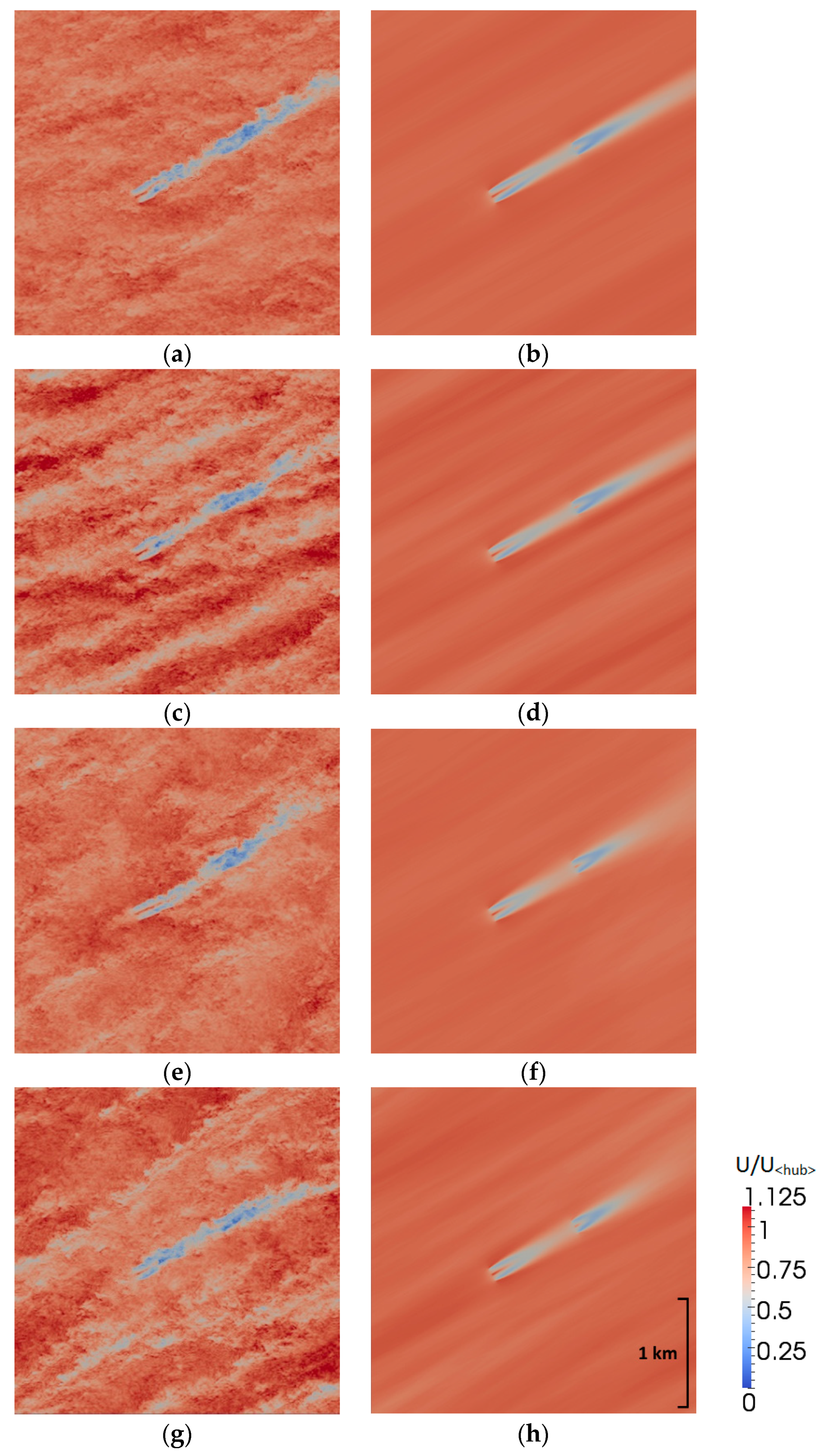
Figure 5.
Top view of the instantaneous (a,c,e,g) and time-averaged (b,d,f,h) vertical velocities for NLABL, NHABL, ULABL, and UHABL (refer to Table 1) at hub-height (Z = 90 m).
Figure 5.
Top view of the instantaneous (a,c,e,g) and time-averaged (b,d,f,h) vertical velocities for NLABL, NHABL, ULABL, and UHABL (refer to Table 1) at hub-height (Z = 90 m).

Figure 6.
Streamwise view of the instantaneous and time-averaged streamwise velocities for NLABL (a,b), NHABL (c,d), ULABL (e,f), and UHABL (g,h) along the centerline. Refer to Table 1 for acronyms.
Figure 6.
Streamwise view of the instantaneous and time-averaged streamwise velocities for NLABL (a,b), NHABL (c,d), ULABL (e,f), and UHABL (g,h) along the centerline. Refer to Table 1 for acronyms.

Figure 7.
Streamwise cut of the turbulent kinetic energy (TKE) contours for (a) NLABL, (b) NHABL, (c) ULABL, and (d) UHABL along the centerline. Refer to Table 1 for acronyms.
Figure 7.
Streamwise cut of the turbulent kinetic energy (TKE) contours for (a) NLABL, (b) NHABL, (c) ULABL, and (d) UHABL along the centerline. Refer to Table 1 for acronyms.

Figure 8.
(a) Horizontal and (b) vertical profiles of TKE.

Figure 9.
TKE at blade tip at maximum height (Z/D = 1.21).

Figure 10.
Reynolds shear stress for (a) horizontal profiles of <u′v′> and (b) vertical profiles of <u′w′> normalized by the mean velocity at hub-height (8 m/s). Turbines positions are indicated with black dashed-lines.
Figure 10.
Reynolds shear stress for (a) horizontal profiles of <u′v′> and (b) vertical profiles of <u′w′> normalized by the mean velocity at hub-height (8 m/s). Turbines positions are indicated with black dashed-lines.

Figure 11.
Time series of the power signals for upstream (WT1) and downstream (WT2) turbines: (a) NLABL, (b) NHABL, (c) ULABL, and (d) UHABL. Refer to Table 1 for acronyms.
Figure 11.
Time series of the power signals for upstream (WT1) and downstream (WT2) turbines: (a) NLABL, (b) NHABL, (c) ULABL, and (d) UHABL. Refer to Table 1 for acronyms.

Figure 12.
(a) Power root mean square (RMS) and (b) time-averaged power for NLABL, NHABL, ULABL, and UHABL. Refer to Table 1.
Figure 12.
(a) Power root mean square (RMS) and (b) time-averaged power for NLABL, NHABL, ULABL, and UHABL. Refer to Table 1.


Table 1.
Matrix of atmospheric boundary layer (ABL) test cases depending on surface roughness and atmospheric stability.
Table 1.
Matrix of atmospheric boundary layer (ABL) test cases depending on surface roughness and atmospheric stability.
| Atmospheric Stability | Surface Roughness | |
|---|---|---|
| Low | High | |
| Neutral | NLABL | NHABL |
| Unstable | ULABL | UHABL |
© 2018 by the authors. Licensee MDPI, Basel, Switzerland. This article is an open access article distributed under the terms and conditions of the Creative Commons Attribution (CC BY) license (http://creativecommons.org/licenses/by/4.0/).
Share and Cite
MDPI and ACS Style
Lee, S.; Vorobieff, P.; Poroseva, S. Interaction of Wind Turbine Wakes under Various Atmospheric Conditions. Energies 2018, 11, 1442. https://doi.org/10.3390/en11061442
AMA Style
Lee S, Vorobieff P, Poroseva S. Interaction of Wind Turbine Wakes under Various Atmospheric Conditions. Energies. 2018; 11(6):1442. https://doi.org/10.3390/en11061442
Chicago/Turabian StyleLee, Sang, Peter Vorobieff, and Svetlana Poroseva. 2018. "Interaction of Wind Turbine Wakes under Various Atmospheric Conditions" Energies 11, no. 6: 1442. https://doi.org/10.3390/en11061442
Note that from the first issue of 2016, this journal uses article numbers instead of page numbers. See further details here.