A Dimensionless Parameter Analysis of a Cylindrical Tube Electromagnetic Vibration Energy Harvester and Its Oscillator Nonlinearity Effect

Abstract

This paper investigates a single degree of freedom oscillator in a cylindrical tube vibration energy harvester which is applicable in a low-frequency range. A duffing-type nonlinear dynamic differential equation of the oscillator was developed for the nonlinear analysis and solved by using the harmonic balance method in order to widen energy harvesting frequency bandwidth. The exploitation of nonlinear spring force interactions of the oscillator to enhance the generator’s performance is also presented in this paper. The dimensionless harvested power formula of the nonlinear mass-spring-damper system was derived, and a parameter study was conducted for the design optimization of the harvester. The main contribution of this paper is to establish a dimensionless performance analysis method of a nonlinear electromagnetic vibration energy harvester system and to disclose the effects of the parameters and nonlinearity of the system on the harvesting performance.

1. Introduction

Vibration energy harvesting has been the subject of many research activities over the last decade. Conversion of kinetic energy in the form of vibrations into electric energy is a very promising way for improving energy utilization. Vibration energy was typically converted into electrical energy using electromagnetic [1,2,3,4], electrostatic [5,6,7] and piezoelectric [8,9] energy conversion transducers. Most of the energy harvesting technologies have converted waste vibration energy into useful electrical energy for replacing or charging the batteries of wireless sensor networks (WSN), and most of the electromagnetic conversion technologies have significant design flexibility to convert vibration energy with large amplitudes. In contrast to this advantage, piezoelectric vibration energy converters are in most cases based on simply supported beams and piezoelectric elements. A piezoelectric vibration energy harvester is more suitable for high frequency, small amplitude vibration energy which has high power density. An electromagnetic vibration harvester is more suitable for low frequency, large amplitude vibration energy which has relatively low power density [10,11].

The most common systems of the linearly modelled mass-spring-damper oscillator were not well-suited for vibration energy harvesting because the output power of a linear vibration energy harvester dropped dramatically under off-resonance conditions [12]. This problem can be overcome by using wide-frequency band mechanisms, such as an array of energy harvesters. Sari developed a harvester generator covering a wide-frequency band of external excitations by implementing a number of serially connected cantilevers of different lengths, resulting in varying natural resonant frequencies [13]. Nevertheless, the adjustment of length increments is hard and cumbersome, and it also decreases power density. Using mechanical stoppers is another way to do this. Soliman produced a piecewise linear oscillator as the energy harvesting element of micro-power generators (MPGs), which increased the energy harvesting frequency bandwidth of the MPG during a frequency up-sweep while maintaining the same bandwidth in a down-sweep [14]. Using nonlinear springs is another option for wide-frequency band tuning. Nguyen proposed an experimental device of the vibration energy harvester which displayed a strong softening spring effect. For narrow-band random excitation, the energy harvester exhibited a widening frequency bandwidth during frequency down-sweeps. For increasing levels of broadband random noise excitation, the energy harvester displayed a broadening frequency bandwidth response. Furthermore, the vibration energy harvester with the softening spring effect not only increased the frequency bandwidth but also harvested more output power than a linear vibration energy harvester under a sufficient level of broadband random excitation. It was found that the bandwidth of a nonlinear vibration energy harvester can increase by more than 13 times and its average harvesting output power can increase by 68% compared to those of a linear vibration energy harvester [15]. It is worth mentioning the interesting concept of a ring magnet added in the surrounding area of the moving magnet, leading to additional nonlinear stiffness to increase power [16]. Another technique was to use frequency tuning mechanisms [17,18,19]. Wischke presented an electromagnetic vibration scavenger that exhibited a tunable modal resonant frequency. It was demonstrated that in the tuning operation mode, more than 50 μW were scavenged continuously across the feasible frequency range of 20 Hz. Wang [17] proposed a system design of a weighted-pendulum-type electromagnetic generator for harvesting energy from a rotating wheel. Cottone et al. [20] designed a nonlinear vibration energy harvester consisting of clamped–clamped buckled beams combined with a four-pole magnet across a coil. For an optimal excitation acceleration level, this configuration showed 2.5 times wider harvesting frequency bandwidth and higher harvested power than those of a linear vibration energy harvester as compared with the mono-stable regime. Multi-frequency harvesters were developed and characterized by using three-dimensional (3D) excitation at different frequencies [21,22,23]. The 3D dynamic behavior and performance analysis of the device showed that the first vibration mode of 1285 Hz had an out-of-plane motion, while the second and third modes of 1470 and 1550 Hz, respectively, were in-plane at angles of 60° (240°) and 150° (330°) to the horizontal (x-) axis. For an input sine wave acceleration excitation with an amplitude of 1 g, the maximum power densities achieved were 0.444, 0.242, and 0.125 μW cm⁻³ at different vibration modes. The flux change rate was not necessarily the largest in this situation and was influenced by the arrangement of magnets and coils [1].

However, most of the proposed wideband energy harvesters operated at relatively high frequencies. In order to match the low resonant frequency with the excitation frequency associated with human motions, i.e., less than 10 Hz, a very compliant spring structure should be adopted, which requires enough space to permit large mechanical displacement to avoid any damage.

In addition to the above literatures for widening harvesting frequency bandwidth, more literatures are categorized into five catalogues of the widened bandwidth harvesters and listed in

Table 1. Relevant literature for five different catalogues.

Year	Harvester Array	Mechanical Stoppers	Nonlinear Springs	Frequency Tuning Mechanisms	Multi-Frequency Harvesters
2002					Ching, N.N., et al. [24]
2003	Mizuno, M. and Chetwynd, D.G. [25]
2005		Priya, S. [26]
2006	Shahruz, S. [27,28]	Rastegar, J., et al. [29] Tieck, R., et al. [30]		Leland, E.S. and Wright, P.K. [31] Spreemann, D., et al. [32]
2007				Hu Y., et al. [33]
2008	Xue, H., et al. [34] Ferrari, M., et al. [35] Sari, I., et al. [13] Liu, J.-Q., et al. [36]	Soliman, M., et al. [14]	Challa, V.R., et al. [37] Ramlan, R., etal. [38] Burrow, S., et al. [39]	Morris, D.J., et al. [40] Eichhorn, C., et al. [41]	Kulkarni, S., et al. [1]
2009	Yang, Z. and Yang, J. [42]		Mann, B., et al. [43] Xing, X., et al. [44] Reissman, T., et al. [45] Erturk, A., et al. [46] Marinkovic, B. and Koser, H. [47] Stanton, S.C., et al. [48]		Yang B., et al. [23]
2010			Dallago, E., et al.[49]	Zhu, D., et al. [19] Wischke, M., et al. [18] Youngsman, J.M., et al. [50]
2012		Liu, H., et al. [51]	Foisal, A.R.M., et al. [52]		Liu, H.,et al. [22]
2013			Munaz A., et al. [53]	Wang, Y.-J., et al. [17]	El-Hebeary, M.M., et al. [54] Liu, H., et al. [21] Ashraf, K., et al. [55]
2014		Borowiec, M., et al. [56]		Cottone, F., et al. [20]
2015	Bendame, M.,et al. [57]		Berdy, D.F., et al. [58]
2016			Masuda, A.; Sato, T. [59] Nammari, A., et al. [60]
2017	Malaji, P.V. and Ali, S.F. [61]		Salauddin, M., et al. [62]

. The five catalogues are harvester array, mechanical stoppers, nonlinear springs, frequency tuning mechanisms, and multifrequency harvesters. A few typical piezoelectric literatures are marked in red. It is seen from the table that the most recent researches are focused on mechanical stoppers and nonlinear springs. Most of studies so far have been conducted to explore the unique characteristics of nonlinear springs to enhance vibration energy harvesting performance.

This paper aims to develop a cylindrical tube electromagnetic vibration energy harvester which collects low-frequency and large-amplitude vibration. Theoretical analysis and experiments of the electromagnetic vibration energy harvester will be conducted, and the major system parameters will be identified. The simulation model of the harvester will be developed and validated by the experimental results. A nonlinear stiffness term will then be included in the validated simulation model. The new simulation results considering nonlinearity will be used to validate the theoretical analysis model with the nonlinear stiffness term. The validated theoretical analysis model will then be used to conduct a parameter sensitivity study of the cylindrical tube electromagnetic vibration energy harvester system.

The relative displacement and output voltage versus the excitation frequency will be calculated and plotted for different system parameter changes, such as the input excitation displacement amplitude z₀, the electromagnetic coupling coefficient Bl, the damping coefficient c, the nonlinear stiffness coefficient k₃, and the external load resistance R. A dimensionless analysis method of a nonlinear electromagnetic vibration energy harvester system will be developed and the effects of the parameters and nonlinearity on the harvesting performance of the system will be studied. The motivation of this paper is to develop a parametric simulation model and optimal design of the harvester system to enable the system to harvest more power and to widen the harvesting frequency band.

2. Analysis of Single-Degree-of-Freedom (SDOF) Nonlinear Cylindrical Tube Electromagnetic Vibration Energy Harvester Using the Time Domain Integration Method

The equation that describes the dynamics of a general nonlinear oscillator can be written as

$$m\times \ddot{x}+c\times \dot{x}+\frac{\mathrm{d}U(x)}{\mathrm{d}x}+\alpha \times V=-m\times \ddot{z}$$

(1)

where m is the mass of the oscillator; c is the damping coefficient; α is the equivalent force factor; x is the relative displacement of the oscillator with respect to the base; $\dot{x}$ and $\ddot{x}$ are the relative velocity and acceleration of the oscillator with respect to the base; z is the base excitation displacement; $\ddot{z}$ is the acceleration of the base excitation; and U(x) is the potential energy of the spring element. V is the voltage across the external load resistance on the two output terminals of the circuit. The nonlinearity of Equation (1) could be caused by the spring force nonlinearity. There is one condition of a nonlinear oscillator that is different from that of a linear one, that is, for a nonlinear oscillator, the potential energy of the spring is given by

$$U(x)\ne \frac{1}{2}\times k\times x^2$$

(2)

where k is the spring stiffness coefficient of the linear displacement term of the oscillator. This means that the potential energy of a nonlinear oscillator is not proportional to a quadratic of the displacement. For the potential energy function U(x), there were some expressions presented in the literature [63], which are given by

$$U(x)={\displaystyle \sum _{n=1}^n\frac{1}{2n}\times k_{2n-1}\times x^{2n}}$$

(3)

where k_2n−1 is the spring stiffness coefficient of linear or nonlinear displacement term or the potential energy coefficient of the nonlinear oscillator and n = 1, 2, 3, … is the integer. For a Duffing-type oscillator, the potential energy function can be defined as

$$U(x)=\frac{1}{2}\times k_1\times x^2+\frac{1}{4}\times k_3\times x^4$$

(4)

where k₁ is the spring stiffness coefficient of the linear displacement term and k₃ is the spring stiffness coefficient of the nonlinear displacement term. k₁ and k₃ are the potential energy coefficients of the nonlinear oscillator.

A typical cylindrical tube Single-Degree-Of-Freedom (SDOF) generator is suspended by two long strings and excited by a vibration exciter as shown in Figure 1, where a cylindrical oscillator of properly stacked magnets slides freely inside the tube and four coils are wrapped on the outer surface of the tube and separated by a distance of the oscillator axial length. There are two fixed magnets in the two end caps of the tube which have opposite polarities to those of the oscillator magnets. The magnetic fields between the magnets in the end caps and the oscillator magnets act as nonlinear magnetic springs for the nonlinear oscillator and the stiffness coefficient could be changed by using different sizes of magnets. Four sets of the coils are shown in the middle of the tube.

The displacement of the tube is assumed to be z, which is the displacement amplitude of the shaker excitation. The displacement of the oscillator is assumed to be y, so the relative displacement of the oscillator with respect to the tube is then equal to y − z. For the study object of the oscillator, it is subjected to the elastic restoring force of the magnetic spring, which is written as $F_k=-k_1\times (y-z)-k_3\times {(y-z)}^3$, and the total damping force of the magnetic spring, which is written as $F_c=-c\times (\dot{y}-\dot{z})$. The electromagnetic force from the coils wired on the outside surface of the tube carrying current is written as $F_e=-Bl\times I$. From Newton’s second law, the dynamic differential equation of the Duffing-type oscillator is given by

$$m\times \ddot{y}+k_1\times (y-z)+k_3\times {(y-z)}^3+c\times (\dot{y}-\dot{z})+Bl\times I=0$$

(5)

where m is the mass of the oscillator; k₁ is the linear spring constant; k₃ is the nonlinear spring constant; c is the damping coefficient; B is the magnetic flux density; I is the current in the coils; l is the total length of the coils where $l=\pi \times D_0\times N$. N is the number of turns in each coil; and D₀ is the outer diameter of the tube. The coils are connected in series to an external resistance R. The series of connected coils have an internal resistance of R_e and an inductance of L_e. The dynamic differential equation of the circuit of the coils is given by

$$V+L_e\times \dot{I}-Bl\times (\dot{y}-\dot{z})=0$$

(6)

Equations (5) and (6) can be solved by using the integration method. Equations (5) and (6) can be written as

$$\{\begin{array}{l}(\ddot{y}-\ddot{z})=-\frac{c}{m}\times (\dot{y}-\dot{z})-\frac{k_1}{m}\times (y-z)-\frac{k_3}{m}\times {(y-z)}^3-\ddot{z}-\frac{Bl}{m\times (R+R_{\mathrm{e}})}\times V\\ \dot{V}=-\frac{R+R_{\mathrm{e}}}{L_{\mathrm{e}}}\times V+\frac{Bl\times (R+R_{\mathrm{e}})}{L_{\mathrm{e}}}\times \dot{x}\end{array}$$

(7)

Equation (7) can be wired and programmed as a code in Matlab Simulink (R2017b, Mathworks, Natick, MA, USA), as shown in Figure 2.

With the given input acceleration excitation of the tube, the output time response of the relative displacement of the oscillator with respect to the tube and the voltage of the two terminals of the circuit can be predicted. The parameters of the tube system such as m, k₁, k₃, c, B, l, and R can be identified and measured from experiments.

It is seen from Figure 2 that if the base acceleration $\ddot{z}$ is fed as a sine wave into the system, the time trace outputs of the relative displacement response (y − z) and output voltage V can be solved and scoped. With inputs of different excitation frequencies and the amplitude of the tube acceleration $\ddot{z}$, or even with the inputs of the real time measured base vibration acceleration, the output voltage and power can also be calculated from the Matlab Simulink code in Figure 2, where the base acceleration sine wave input should be replaced with a measured excitation data file. In the above calculations, the inductance L_e can be calculated by

$$L_{\mathrm{e}}=\pi \times {\mu }_0\times {\mu }_r\times \frac{N^2\times D_0^2}{4\times h_c}$$

(8)

where μ₀ = 4π × 10⁻⁷ N·m⁻² is the permeability of the coil with air core; μ_r is the permeability coefficient of the coil, for the iron core, μ_r = 1450, for the air core, μ_r = 1; π = 3.1415926; D₀ is the diameter of the tube; and h_c is the height of each coil. The magnetic flux density B can be either measured in experiments using a Gauss meter or calculated by the simulation using numerical tools such as ANSYS Maxwell (Release 16.0.2, Ansys, Inc, Canonsburg, PA, USA), which is based on the calculated average magnetic flux density of the multiple points in the magnetic field around the coil [43,46,64]. With inputs of different values of external resistance R, inductance L_e, the magnetic flux density B, and the total length of the coil wire l, the output voltage and power can be calculated and optimised.

Equations (5) and (6) can also be solved using the harmonic balance method, which is illustrated below.

3. Dimensionless Analysis of the Nonlinear Cylindrical Tube Electromagnetic Vibration Energy Harvester Using the Harmonic Balance Method

In this section, a nondimensional analysis method is developed to investigate the characteristics of the proposed energy harvester, although the dimensionless performance analysis of nonlinear electromagnetic vibration energy harvesting was also conducted by [64,65]. In order to solve Equations (5) and (6), it is assumed that

$$x=x_0\times \cos (\omega t) V=V_0\times \cos \left(\omega t+{\phi }_1\right) z=z_0\times \cos \left(\omega t+{\phi }_2\right)$$

(9)

where x = y − z is the relative displacement of the magnet oscillator with respect to the tube; x₀ is the amplitude of x; ω is the excitation frequency of the tube; t is the time variable; V is the output voltage of the coils connected in series to an external resistance R; V₀ is the amplitude of V; ϕ₁ is the phase difference between the output voltage V and the relative displacement x; z is the excitation displacement of the tube; z₀ is the amplitude of z; and ϕ₂ is the phase difference between the tube excitation displacement z and the relative displacement x. Substituting Equation (9) into Equation (6) gives

$$V_0=\frac{Bl\times \omega \times x_0}{\sqrt{{\left(\frac{L_{\mathrm{e}}}{R}\times \omega \right)}^2+1}}$$

(10)

It can be assumed that

$$A={\omega }^2\times z_0 \alpha =\frac{Bl}{R}$$

(11)

Substituting Equation (9) into Equation (5) provides

$$x_0^2=\frac{A^2}{{\left({\omega }^2-\frac{k_1}{m}-\frac{3}{4}\times \frac{k_3}{m}\times x_0^2-\frac{L_{\mathrm{e}}\times B^2{l}^2\times {\omega }^2}{\left(L_{\mathrm{e}}^2\times {\omega }^2+R^2\right)\times m}\right)}^2+{\left(\frac{B^2{l}^2\times R\times \omega }{\left(L_{\mathrm{e}}^2\times {\omega }^2+R^2\right)\times m}+\frac{c}{m}\times \omega \right)}^2}$$

(12)

It can be assumed that

$$\begin{array}{c}{\omega }_{\mathrm{N}}=\sqrt{\frac{m}{k_1}}\times \omega ;\xi =\frac{c}{2\times \sqrt{m\times k_1}};M^2=\frac{k_3}{k_1}\times x_0{}^2;\hfill \\ f{f}^2=\frac{m^2\times k_3}{k_1^3}\times A^2=\frac{m^2\times k_3}{k_1^3}\times {\omega }^4\times z_0^2;\sigma =\frac{B^2{l}^2}{k_1};k_{\mathrm{R}}=\sqrt{\frac{m}{k_1}}\times R; \beta =\frac{k_3}{k_1}\hfill \end{array}$$

(13)

From Wang X., et al. [66], the normalized dimensionless resistance R_N and force factor α_N are given by

$$\{\begin{array}{l}{R}_{\mathrm{N}}=\frac{R}{L_{\mathrm{e}}\times \omega }\\ {\alpha }_{\mathrm{N}}=\sqrt{\frac{{\alpha }^2\times L_{\mathrm{e}}\times \omega }{c}}=\frac{B\times l}{R}\times \sqrt{\frac{L_{\mathrm{e}}\times \omega }{c}}\end{array}$$

(14)

Substituting Equations (13) and (14) into Equation (12) gives

$$M^2=\frac{f{f}^2}{{\left({\omega }_{\mathrm{N}}^2-1-\frac{3}{4}\times M^2-\frac{2\times \xi \times R_{\mathrm{N}}^2\times {\omega }_{\mathrm{N}}\times {\alpha }_{\mathrm{N}}^2}{1+R_{\mathrm{N}}^2}\right)}^2+{\left(\frac{2\times \xi \times R_{\mathrm{N}}^3\times {\alpha }_{\mathrm{N}}^2\times {\omega }_{\mathrm{N}}}{1+R_{\mathrm{N}}^2}+2\times \xi \times {\omega }_{\mathrm{N}}\right)}^2}$$

(15)

where M is the response amplitude of the system. It is noted that Equation (15) is cubic in M². Thus, there are three or one-real root(s) for a given frequency.

Differentiating both the sides of Equation (15) with respect to frequency ω_N and assuming that ξ is a constant, and when $\frac{\partial M}{\partial {\omega }_{\mathrm{N}}}\to \infty$, there are two jump points in the frequency response curve and it is an undetermined region between the two jump points.

From Equations (11)–(14), it gives

$$\frac{x_0}{z_0}=\frac{{\omega }_{\mathrm{N}}^2}{\sqrt{{\left[1+\frac{3}{4}\times M^2+\left(\frac{2\times \xi \times R_{\mathrm{N}}^2\times {\omega }_{\mathrm{N}}\times {\alpha }_{\mathrm{N}}^2}{1+R_{\mathrm{N}}^2}-{\omega }_{\mathrm{N}}^2\right)\right]}^2+{\left(2\times \xi \times {\omega }_{\mathrm{N}}+\frac{2\times \xi \times R_{\mathrm{N}}^3\times {\alpha }_{\mathrm{N}}^2\times {\omega }_{\mathrm{N}}}{1+R_{\mathrm{N}}^2}\right)}^2}}$$

(16)

From Equations (10) and (16), it gives

$$\begin{array}{ll}\frac{V_0}{Bl\times \omega \times z_0}=& \frac{1}{\sqrt{1+R_{\mathrm{N}}^2}}\hfill \\ & \times \frac{{\omega }_{\mathrm{N}}^2}{\sqrt{{\left[1+\frac{3}{4}\times M^2+\left(\frac{2\times \xi \times R_{\mathrm{N}}^2\times {\alpha }_{\mathrm{N}}^2\times {\omega }_{\mathrm{N}}}{1+R_{\mathrm{N}}^2}-{\omega }_{\mathrm{N}}^2\right)\right]}^2+{\left(2\times \xi \times {\omega }_{\mathrm{N}}+\frac{2\times \xi \times R_{\mathrm{N}}^3\times {\alpha }_{\mathrm{N}}^2\times {\omega }_{\mathrm{N}}}{1+R_{\mathrm{N}}^2}\right)}^2}}\hfill \end{array}$$

(17)

and the harvested power is given by

$$\begin{array}{ll}\frac{P_{\mathrm{h}}}{\left(\frac{m^2\times z_0^2\times {\omega }^4}{c}\right)}& =\frac{4\times {\omega }_{\mathrm{N}}^2\times {\xi }^2\times R_{\mathrm{N}}^{}\times {\alpha }_{\mathrm{N}}^2}{\left[1+R_{\mathrm{N}}^2\right]}\hfill \\ & \times \frac{1}{{\left[1+\frac{3}{4}\times M^2+\left(\frac{2\times \xi \times R_{\mathrm{N}}^2\times {\alpha }_{\mathrm{N}}^2\times {\omega }_{\mathrm{N}}}{1+R_{\mathrm{N}}^2}-{\omega }_{\mathrm{N}}^2\right)\right]}^2+{\left(2\times \xi \times {\omega }_{\mathrm{N}}+\frac{2\times \xi \times R_{\mathrm{N}}^3\times {\alpha }_{\mathrm{N}}^2\times {\omega }_{\mathrm{N}}}{1+R_{\mathrm{N}}^2}\right)}^2}\hfill \end{array}$$

(18)

Dimensionless harvested voltage and power ratios for the nonlinear oscillator as shown in Equations (17) and (18) are comparable to those for the linear electromagnetic and piezoelectric [66,67,68]. For the nonlinear oscillator, in addition to the dimensionless control variables of R_N and α_N, the mechanical damping ratio ξ and dimensionless relative displacement of the oscillator M are also control variables of the dimensionless harvested voltage and power ratios, which is different from that of the linear oscillator. Equations (17) and (18) are applicable to many similar vibration energy harvesters regardless of their design sizes.

4. Experimental Investigation and Parameter Study of a Cylindrical Tube Electromagnetic Energy Harvester

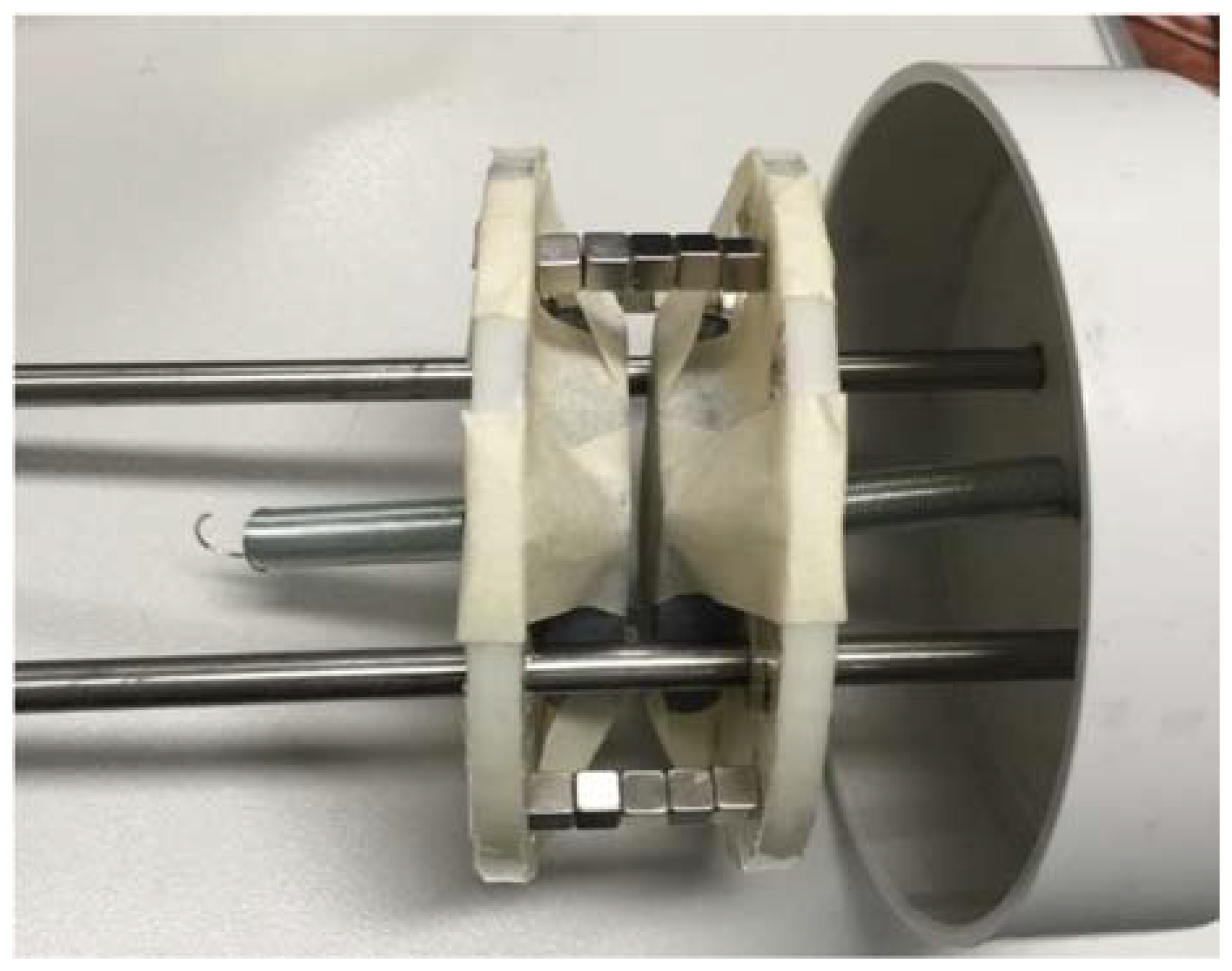
The general idea behind this device is that the tube moving back and forth will cause the magnets to move and pass the coils, which will cut the magnetic flux and produce an electrical current. In order to identify the system parameters for analysis and simulation, a cylindrical tube electromagnetic energy harvester was designed and constructed, as shown in Figure 3. Two 5 mm thick, 96 mm diameter disks were slid into the tube. The two disks were separated and tied together by five stacks of magnets. A 100 mm diameter and 200 mm length Polyvinyl chloride (PVC) tube was used to house the assembly of the disks and the support rods. The PVC tube had two end caps where the two support rods were attached through and fixed onto by the end threads of the rods and nuts. Each of the end caps was fitted with a magnet which had the opposite polarity to that of the disk on either of the tube sides. Therefore, a magnetic spring was formed between each of the disks and each of the end caps on either of the tube sides. Alternatively, for a linear oscillator, two identical steel springs were used to connect the disks and the end caps of the tube. In this case, one spring was used to connect one disk at one end and one end cap at the other end. The other spring was used to connect the other disk to the other end cap of the tube. These springs were symmetrically installed on both sides of the tube, as shown in Figure 3. The disk assembly inside the tube formed the magnet oscillator which would hover on the rods and rebound with oscillation. WD40 lubricant was applied onto the surface of the rods, which helped to reduce friction and enhance energy harvesting efficiency. In order to reduce the natural frequency of the magnet oscillator, a weight was added to each of the disks which would increase the inertia of the magnet oscillator and allow for a larger rebound or oscillation (Figure 3). Each of the disks was inserted with 20 pieces of 5 × 5 × 5 mm neodymium magnets in an 80 mm diameter ring array, as shown in Figure 4, where the two holes in the disk were used to mount the disk onto the two support rods. The magnets were arranged in the Halbach array pattern in the circumference direction so that the fluxes were oriented outward in the radial direction of the tube and the direction of the coil wiring was perpendicular to that of the fluxes. Ideally, the magnets inserted inside the disks should be arranged in a straight line rather than in a ring, with the poles of the magnets arranged in a Halbach array pattern. The larger the disk diameter is, the less the pattern error there is. When the disk diameter tends to be infinite, the pattern error tends to be zero. The effect of the circumferential gap between two nearby magnets on the magnetic field intensity around the two magnets can also be simulated using ANSYS Maxwell and Simplorer and Electromagnetics (Release 16.0.2, Ansys, Inc, Canonsburg, PA, USA) and is shown in Figure 4. The magnets stacked up in the axial direction between the two disks as shown in Figure 3 were not used for energy harvesting but were used to separate the two disks, which had little effect on the energy harvesting performance.

The Maxwell simulation of the Halbach and alternating transverse polarity arrangements was simplified by adopting 12 magnets instead of 20 magnets, which should demonstrate the same flux distribution trend of adopting 12 magnets as that of adopting 20 magnets. The magnetic flux distributions of the topological opening up of the magnet ring array (north outward) are compared for the Halbach and alternating transverse polarity arrangements in Figure 4. It is seen from Figure 4 that the magnetic field intensity outside the disk in the Halbach arrangement is larger than that on either side of the disk in the alternating transverse polarity arrangement. Therefore, the Halbach magnet arrangement is better than the alternating transverse polarity magnet arrangement for enhancing magnetic field intensity. It is also seen from Figure 4 that the top side of the topological opening up of the ring array has much larger magnetic field intensity than the bottom side. Therefore, the outside of the disk had much higher magnetic field intensity than the inside. The marked red arrows beside the magnets on the disk pointed to their north polarities. The rare earth magnets were arranged in a Halbach array and inserted onto the disks, which would maximize the strength of the magnetic field outside the disk where 0.5 mm gauge copper coils were wound around the outer surface of the tube. Four coils of 65 turns were separated from each other for a distance of 15 mm. Each set of the coils was connected to a bridge rectifier to convert AC current into DC current, which facilitates the connections in the series. The four coils were connected in series for their output. The Maxwell transient simulation was also conducted to compare which magnet arrangement creates more current in the same circuit situation. It was found that the Halbach magnet arrangement creates more current than the alternating transverse polarity magnet arrangement.

4.1. Experimental Results and Parameter Study of the Linear Oscillator System

In order to verify the simulation results, an experimental system was developed and tested. As shown in Figure 5, the vibration energy harvester or the cylindrical tube generator was suspended by two fine ropes to a fixed end. The vibration energy harvester was connected to the vibration exciter through a fine rod and horizontally excited by the shaker, as shown in Figure 5. The measurement data was recorded and analyzed by a computer data acquisition and analysis system. For the linear oscillator, the fixed magnets in the end caps were removed and two steel springs were used to connect the disks to the end caps. The output AC voltage signal was measured and recorded by the computer data acquisition frontend. The device was excited by the PC-controlled shaker, which was driven by a Polytec laser vibro-meter system through a power amplifier.

When the tube pendulum was swayed, the magnet oscillator inside the tube would have moved fore and aft passing the coils. The coils would have cut the magnetic flux, which would induce a current.

4.2. Parameter Identification

In order to identify the stiffness and damping coefficients of the magnetic springs, the ANSYS Maxwell and Electromagnetics software was used to simulate the magnetic field between the disks and end caps for calculation of the restoring force of the magnetic springs versus the displacement of the magnet oscillator. It was assumed that the magnet oscillator was the Duffing-type oscillator. Therefore, the linear and nonlinear stiffness coefficients of the magnetic springs, k₁ and k₃, can be identified from the least-squares curve fitting of the simulation data of the restoring force and displacement of the oscillator. The magnetic flux density B can be calculated from the magnetic field simulation or can be measured from the device using a Gauss meter for the average value of many points in the magnetic field. The total length l of the coil can be measured by a rule. Therefore, Bl can be calculated from multiplying B by l. The inductance of the coils L_e can be calculated from Equation (8).

In order to identify the system parameters for the theoretical analyses and calculations, as well as the simulation for the output voltage and harvested power of the electromagnetic harvester, the experimental system shown in Figure 5 had to be physically tested. A swept sine (or white noise) signal was used to excite the pendulum tube with the displacement amplitude of 0.8 mm and the output voltage frequency response function amplitude of the coils was measured and is shown in Figure 6a. From the modal resonant peak of the frequency response function amplitude curve, the natural frequency of the oscillator was identified. From the mass measured and natural resonant frequency identified, the stiffness coefficient of the steel springs can be calculated. The damping ratio was identified from the modal resonant peak using the half-power bandwidth method, from which the damping coefficients of the system were calculated from the measured mass, the identified damping ratio, and natural resonant frequency. It is seen that the output voltage results of the simulation and experiment measurement coincide well in the frequency range from 0 Hz to 10 Hz. Above 10 Hz, the experimental measurement output voltage results have large error bar ranges. The output voltage results are largely reduced. There are two possibilities which would cause the large error bar range of the measured voltage above 10 Hz. One possibility is that the misalignment of the stacked-up magnets between the two disks would cause the other modes of vibration, which was not accounted for in the prediction model. The other possibility is that the relative motion of the oscillator with respect to the base tube could be sometimes zero or sometimes, nonzero, which is in a nonstable state generating a large friction force between the disk and supporting rail rods. This is because in the experiments, at off-resonances, the structure was not steadily oscillating in the axial direction, which may lead to a static friction force between the two disks and supporting rail rods. When the frequency increases above 10 Hz, the relative motion of the oscillator with respect to the base tends to less than that at the resonance and tends to be very small. In other words, when the frequency increases, the oscillator tends to be static and the base excitation tends to move the oscillator again. The static friction force at off-resonances is much larger than the sliding friction force between the two disks and supporting rods at the resonance. Therefore, the equivalent damping coefficients at the off-resonances are much larger than the damping coefficient at the resonance in the experiments. In the simulation, the damping coefficient is assumed to be constant and equal to the resonant damping coefficient in the whole frequency range. The off-resonance damping coefficients were up to around 4 times the resonant damping coefficient. This has explained how the large error range was developed above 10 Hz in Figure 6a.

The first possibility can be eliminated by a bolted connection of six aluminium tubes between the two disks as mentioned before. The second possibility can be eliminated by adding lubricating oil on the supporting rail rods. The root causes of the large error bar range of the measured voltage will be sorted out in our future work.

The measured, identified parameters of the oscillator are listed in

Table 2. Identified parameters of the oscillator.

Parameters	Values
k1 (N/m)	1010.6
k3 (N/m3)	125,000
m (kg)	0.4
c (Ns/m)	6
Bl (Tm)	0.064
Le (H)	0.0051
Re (Ohm)	8
Ri (Ohm)	8
z0 (mm)	0.8

. In order to verify the identified oscillator parameters, a sine wave excitation was generated where the excitation frequency of the shaker was set to be close to the resonant frequency of the oscillator and the voltage output was measured. The excitation displacement amplitude was varied, the excitation frequency was fixed at the resonant frequency, and the other parameters in Table 2 were not changed. The output voltage was measured and compared with the simulation results with error bars as shown in Figure 6b. The measured output voltage in Figure 6a,b was the open circuit voltage. When the external load resistance was applied and varied, the excitation frequency was fixed at the resonant frequency and the other parameters in Table 2 were not changed. The output voltage was measured and is shown in Figure 6c, where the simulated voltage has been extended up to 30 Ohm, which tends to saturation according to [46]. This extension should be enough, as the trend has been shown in a range of 0–30 Ohm while the internal resistance is around 8 Ohm, which is in the range for matching the internal and external resistances.

Figure 6 shows the trend of the output voltage for changing the excitation frequency, amplitude, and the external load resistance R. It is clearly seen that the measured and simulated results match with each other very well. The experimental results have verified simulation results. The simulation model has been validated.

4.3. Monte Carlo Simulation and Parameter Sensitivity Study of the Linear Oscillator System

A Monte Carlo simulation is a computerized mathematical technique that allows people to account for risk in quantitative analysis and decision making. Monte Carlo simulation performs risk analysis by building models of possible results by substituting a range of values—a probability distribution—for any factor that has inherent uncertainty. It then calculates results over and over, each time using a different set of random values from the probability functions. Depending upon the number of uncertainties and the ranges specified for them, a Monte Carlo simulation could involve thousands or tens of thousands of recalculations before it is complete. Monte Carlo simulation produces distributions of possible outcome values.

The probability density of the excitation frequency was assumed to be uniformly distributed in the frequency range of 0–30 Hz. The probability density of any one of the parameters, such as the mass, stiffness, damping coefficient, electromechanical coupling coefficient, external resistance, and coil induction (m, k, c, Bl, R, L_e), of the system was assumed to be normally distributed with the mean values of m, k, c, Bl, R, L_e and the standard deviations of 10% of the mean values, respectively. The Monte Carlo simulation results predict the variation range of the output voltage for random excitation frequencies, random excitation displacement amplitude, and random system property parameters. The Monte Carlo simulation results are used to reflect the variation range of the output voltage of a batch of the devices due to the variations of materials and manufacturing processes.

The Monte Carlo simulation results of the output voltage with a parameter variation of 10% were calculated and are plotted in Figure 7. The blue and red dots represented the random output voltage which are higher and lower than the simulated mean output voltage respectively. It is seen from Figure 7a that a damping coefficient variation of (±)10% has very little influence on the output voltage at the off-resonances but has a large influence on the output voltage only at the resonant frequency. An electromechanical coupling coefficient variation of 10% has a large influence on the value of the output voltage from the resonant frequency onward, as shown in Figure 7b. A spring stiffness variation of 10% has an influence on the resonant frequency of the device and has a large influence on the output voltage value around the resonant frequency, as shown in Figure 7c. A mass variation of 10% has an influence on the resonance frequency and has a limited influence on the output voltage of the device around the resonant frequency, as shown in Figure 7d. An external load resistance variation of 10% also has a large influence on the value of the output voltage from the resonant frequency onward, as shown in Figure 7e. A coil induction variation of 10 % has very little effect on the output voltage, as shown in Figure 7f. As the electromechanical coupling coefficient Bl and external load resistance R contribute to the equivalent electric damping, this is why they also have large effects on the resonant output voltage. In summary, the damping coefficient has the largest effect on the resonant output voltage. The electromechanical coupling coefficient Bl has the largest influence on the output voltage at off-resonances.

4.4. Theoretical Analysis, Calculation, and Parameter Study of the Nonlinear Oscillator System

After the simulation model of the linear oscillator system was validated, the nonlinear stiffness k₃ was included in the simulation model shown in Equation (5) and Figure 2, which forms the simulation model of the nonlinear oscillator system. The output voltage versus the excitation frequency was simulated for the nonlinear oscillator system and is plotted in round dots in Figure 8. The simulation results of the nonlinear oscillator system were used to verify the analytical results of the nonlinear oscillator system from Equation (17). The excitation displacement amplitude was 20 mm and the other parameters were identified and are listed in Table 2. The identified nonlinear stiffness coefficient k₃ is 125,000 N/m³. The output voltage versus the excitation frequency is plotted and shown in a solid curve in Figure 8. It is clearly seen that the analytical results match well with the simulation results of the nonlinear oscillator system, which has validated the nonlinear analysis model. Figure 8 aims to study the potential harvesting performance of the nonlinear oscillation harvester using the analysis method, which will provide a guide for its further improvement for different applications.

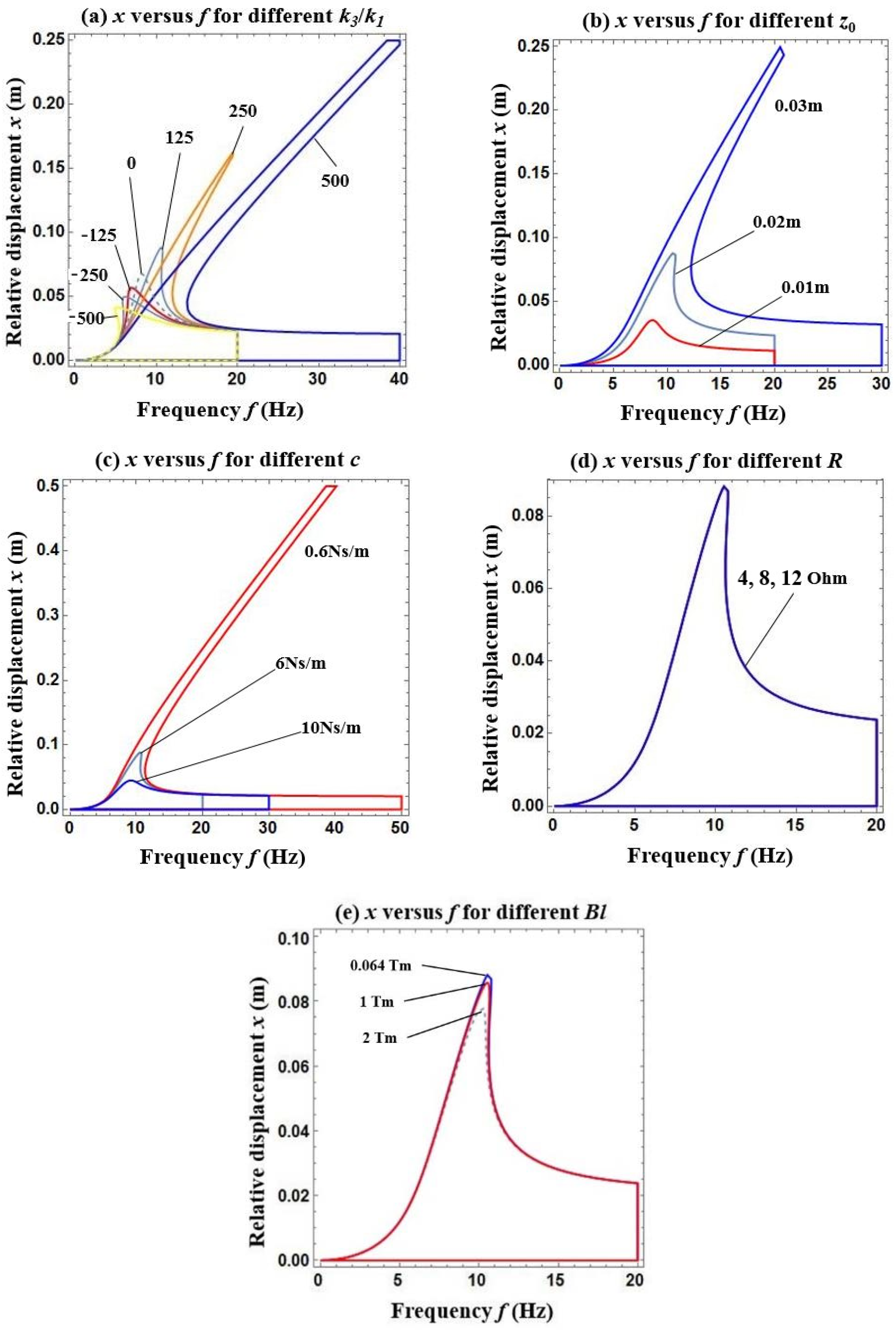
After the analytical model was validated, the analytical model could be used to conduct a parameter study of the nonlinear oscillator harvester system. In order to study the influence of different parameters and the system nonlinearity on the harvesting performance, the relative displacement of the nonlinear oscillator and the output voltage versus the excitation frequency were analytically calculated from Equations (16) and (17) for different system parameters and are plotted in Figure 9 and Figure 10 for comparison. In Figure 9 and Figure 10, the excitation displacement amplitude z₀ is varied for 0.01, 0.02, 0.03 m, the damping coefficient c is varied for 0.6, 6, 10 Ns/m, the external load resistance R is varied for 4, 8, 12 Ohm, the electromechanical coupling coefficient Bl is varied for 0.064, 1, 2 Tm, and the ratio of the nonlinear and linear stiffness coefficients of the magnetic spring k₃/k₁ is varied for ±125 and ±250 m⁻², respectively.

Figure 9a–e shows the relative displacement frequency response by changing the nonlinear stiffness coefficient, base excitation displacement amplitude, damping coefficient, load resistance, and electromechanical coupling coefficient. The largest displacement will occur at the resonance of the nonlinear harvester system, which is different from the resonant frequency of the equivalent linear system. One noticeable change is the significant increase in the relative displacement that is associated with an increase in the nonlinear stiffness coefficient and base excitation displacement amplitude and is also associated with a decrease in damping coefficient and electromechanical coupling coefficient. This is because the electromechanical coupling coefficient is related to the electric damping. Decrease of either mechanical or electric damping will increase the relative displacement of the nonlinear oscillator.

The results shown in Figure 9a–e and Figure 10b–e are based on the assumption that the harvester works in an open circuit. The figures show the sensitivities of the oscillator relative displacement and output voltage to the main parameters. It is seen from the frequency response amplitude curves in Figure 10 that the increased base excitation displacement amplitude and nonlinear stiffness coefficient have developed the multiple periodic attractors and jump phenomena for a strong system nonlinearity. As shown in Figure 10, when the excitation frequency starts from zero and increases along the left-hand side of the curve, the end points of the solid curve near the resonant frequencies are the jumping-down points where $\frac{\partial V}{\partial f}\to \infty$. When the excitation frequency starts from infinity and decreases along the right-hand side of the curves, the end points of the solid curve are the jumping-up points. The jumping-down and jumping-up points are illustrated in Figure 10c. The dash curves in between the jumping-down and jumping-up points is the unstable region. It is well-known that different attractors could coexist for a set of parameters in a nonlinear system [69]. A control strategy on the initial value conditions should be used to extend the harvesting frequency band. However, this control research is out of the scope of this paper. When k₃ is appropriately increased, the system nonlinearity increases dramatically. The system nonlinearity is reflected by the degree of bending of the frequency response amplitude curves, as shown in Figure 9a–c and Figure 10d. The same trend shows that when the mechanical damping coefficient c is small, the nonlinearity is distinct, as shown in Figure 10b. This is because the decreased damping coefficient will increase the vibration amplitude, which is similar to the trend in Figure 10c, and leads to the distinct system nonlinearity. The output voltage values are sensitive to the changes of the damping coefficient and electromechanical coupling coefficient, as shown in Figure 10b,e. These results in Figure 10b,e have the same trends as those in Figure 7a,b. The electromechanical coupling coefficient Bl has a larger effect on the output voltage value than on the relative displacement. In other words, the output voltage value is more sensitive to electromechanical coupling coefficient Bl than to the relative displacement. This is because the electromechanical coupling coefficient Bl is attributed to the added electric damping to the harvester system. Therefore, the electromechanical coupling coefficient Bl and the mechanical damping coefficient c have a similar effect on the output voltage value.

It is seen from Figure 10b–d that the damping coefficient c, the excitation displacement amplitude z₀, and the nonlinear stiffness ratio k₃/k₁ all have large influences on the harvesting performance, including the output voltage and harvesting bandwidth. It is seen from Figure 9d that the external resistance R has very little effect on the relative displacement. It is seen from Figure 10a that the external resistance R has certain influences on the output voltage value. The result in Figure 10a shows the same trend as that in Figure 7e in regard to the sensitivity of the output voltage value to the external load resistance. Similarly, the external resistance R can also be attributed to the added electric damping to the harvester system. The external resistance R and the mechanical damping coefficient c have a similar effect on the output voltage value.

An interesting result from Figure 10 is the extended harvesting bandwidth for the output voltage that is exhibited by enhancing the nonlinearity of the system or more bending of the frequency response amplitude curve, as shown in Figure 10c,d. In essence, Figure 10c,d show that the system nonlinearity could potentially be used to provide a larger output voltage over a wider excitation frequency. The system nonlinearity has widened the harvesting frequency bandwidth through moving the maximum output voltage peak away from the resonant frequency of the equivalent linear system, as shown in Figure 10c,d. In order to achieve the high output voltage, an ideal nonlinear oscillator should have a reasonably large k₃, a relatively low damping coefficient, and an optimised coupling coefficient Bl.

5. Conclusions

In this paper, a cylindrical tube vibration energy harvester is developed and analyzed. The focus is on developing a dimensionless analysis method of a nonlinear cylindrical tube electromagnetic vibration energy harvester which is applicable to many similar vibration energy harvesters regardless of their design sizes. The system parameters have been identified through experiments and finite-element magnet field simulation. The simulation model has been developed and validated by experiments. The analytical model has been developed and validated by the simulation model. The analysis results have been verified by the simulation results using the software Matlab Simulink. The system parameter sensitivity analysis has been conducted through a Monte Carlo simulation for the linear oscillator and through the analytical model for the nonlinear oscillator. It was found that the system nonlinearity could potentially be used to provide a larger output voltage over a wider excitation frequency range. The system nonlinearity can be enhanced through increased nonlinear spring stiffness, decreased mechanical damping, and increased displacement excitation amplitude. The excitation displacement amplitude, the nonlinear stiffness, and the mechanical damping have large influences on the harvested voltage, frequency bandwidth, and oscillator relative displacement. The electromechanical coupling coefficient Bl and the external load resistance R have large influences on the harvested voltage but have small or little influences on the oscillator relative displacement.

This analysis results show a clear direction of the anticipated output voltage through tuning the parameters of the device for design of such the harvesters for a higher efficiency.