3-D EHD Enhanced Natural Convection over a Horizontal Plate Flow with Optimal Design of a Needle Electrode System

Abstract

The present study is intended to investigate the effect of electrohydrodynamic (EHD) enhanced heat transfer on natural convection flow. The flow is assumed to be three-dimensional, turbulent and steady. An experiment was carried out to verify the accuracy of the numerical results and to provide electric properties such as induced current and power consumption to be used as the criteria for the numerical solution procedures. An optimal analysis was carried out along with the simplified conjugate-gradient method, where the objective function was defined as the heat transfer enhancement per input power, which is maximized by searching for the optimum electrode pitch (SL) and height (H) combination. A search for the optimum electrode pitch (SL) and electrode height (H), ranging from 50 mm < SL < 200 mm and 15 mm < H < 55 mm, respectively, with V₀ (12, 14, 16, 18 and 20 kV) and ΔT (33, 53 and 73 K), was performed, respectively. The results showed that the maximum heat transfer enhancement per power consumption reached 4.42–9.72.

1. Introduction

EHD (Electrohydrodynamics) heat transfer enhancement technology is widely used in such devices as heat exchangers, heat recovery devices, air-cooled condensers, evaporators, high thermal wafer cooling systems, micro-pumps, and so on. The main core principle of electrohydrodynamics (EHD) is the mechanism by which an electric field is applied to influence the motion of the flow field. The most commonly working fluid is air. When the voltage exceeds the threshold voltage, air between both ends of the electrodes becomes positive ions due to dissociation, and free electrons cause ion wind in the direction of the electric field. The effect is the added mixing and destabilization of the thermal boundary layer, which results in a substantial heat transfer enhancement.

The first researchers to use EHD to enhance the heat transfer were Marco and Velkoff [1]. They used a wire electrode situated near a vertical plate. They found that the heat transfer enchantment can be up to five times by using EHD technique. O’Brien and Shine [2] presented the EHD heat transfer effect of a vertical plate. The results revealed that the heat transfer coefficient increases with the electrode current. In addition, as the boundary layer thickness decreases, the heat transfer coefficient increases with increases in surrounding pressure. Kibler and Carter [3] investigated a needle electrode system and found that the heat transfer coefficient was proportional to the fourth root of the electrode current. Franke and Hogue [4] proved that for a given current or power level, a needle electrode was more effective than a wire electrode in terms of increasing the heat transfer rate. The natural convection heat transfer rates from a horizontal cylinder can be enhanced 6 times by electrostatic cooling. Owsenek et al. [5] found that at high voltages, negative ions produce less of a drop in the impingement point local heat transfer coefficient. This implies that a negative polarity corona wind generates less Joule heating than a positive corona wind. Thus, a positive corona wind consumes less power and is more efficient than a negative corona wind. Owsenek and Seyed-Yagoobi [6] showed that the heat transfer enhancement for a needle electrode is better than that of a wire electrode by as much as 10 percent for identical power consumption. The upward force above a wire electrode may therefore explain, at least partially, the fact that greater heat transfer enhancement is achieved with needle electrodes than with wire electrodes. Bhattacharyya and Peterson [7] found that the polarity change of the electrode was not found to produce any obvious influence on the heat transfer enhancement ratio. Huang et al. [8] found that when the total corona current exceeds 1 μA, significant heat transfer enhancement is obtained. The heat transfer enhancement is proportional to 1/4 of the power of the corona current for a specific electrode height regardless of electrode placement. Go et al.’s [9] corona discharge experiments proved enhancement of local cooling due to ionized winds. An increase of more than twice the local heat transfer coefficient was observed under typical external forced flow conditions. Jewell-Larsen et al. [10] found the COP of the second generation EHD cooling system to be five times higher than that of the first generation. Shakouri and Esmaeilzadeh [11] visualized the flow patterns in the presence of EHD actuators and found that effect of secondary flow on the recirculation zone or dead zone. The fresh cool air was conducted from the top space of the duct to the hot region by the applied electric field. Peng et al. [12] numerically studied heat transfer enhancement using electrohydrodynamic in a rectangular channel. The results indicated that when the electrode number is more than 7, the heat transfer enhancement reaches a upper limit. In addition, for multiple electrodes, design standard was suggested for the optimal electrode arrangement.

Heidarinejad and Babaei [13] numerically investigated that the induced secondary flow via EHD had a significant effect on water evaporation. Their results showed that the vortex becomes larger at lower Reynolds numbers and that the enhancement of mass transfer factor can exceed its value by as much as 2.25 times with an applied voltage of 20 kV. Leu et al. [14] numerically and experimentally investigated the EHD with mass transfer of forced convection flow in a channel with wire electrodes. The results revealed the EHD effect can effectively enhance water evaporation performance. It is shown that there is an optimal combination of SL and H for different applied voltages. Lai and Shama [15] experimentally evaluated the EHD enhancement of drying rate using multiple electrodes. The results indicated that the drying rate enhancement is increased linearly with the applied voltage. Lin and Jang [16] utilized electrohydrodynamic wire electrodes to numerically study the heat transfer performance of a finned-tube heat exchanger exchangers. It was shown that the area reduction ratio may be up to 56% by using EHD technique.

The foregoing literature review shows that no associated 3-D numerical analysis for the optimization of a needle electrode arrangement on EHD-induced natural convection problems has been conducted. It has motivated the current investigation. In this study, the optimization of electrode pitch and electrode height (longitudinal and transverse distance) is investigated and solved numerically using a commercial ESI-CFD code [17] along with the simplified conjugate-gradient method (SCGM) [18]. For optimal analysis, the heat transfer enhancement per power consumption is defined as the objective function. The influences of electrode pitch (50 mm < SL < 200 mm) and electrode height (15 mm < H < 55 mm) on the heat transfer enhancement and power consumption at different applied voltages (V₀ = 12, 14, 16, 18 and 20 kV) and temperature difference between the wall and ambient (ΔT = 33, 53 and 73 K) are examined. The optimal combination for two operating parameters (SL and H) at a specified applied voltage (V₀) and temperature difference (ΔT) are also obtained.

2. Mathematical Analysis

2.1. Governing Equation

Figure 1 shows the physical model and related geometric dimensions of the natural convection frame with a needle electrode system. The needle electrodes were set above the isothermal wall surface. The distance from electrode tip to the heating plate was defined as the electrode height (H). The distance from electrode to electrode was defined as the electrode pitch (SL). In order to reduce the numerical calculation time, the numerical model was simplified to take the symmetry plane in the transverse face. The length (L_x = 100 mm + 5 × SL) and width (L_w = SL/2) of the isothermal wall surface comprised the heat transfer area (A = L_x × L_w) for different applied voltages (V₀) and temperature difference between the wall and ambient (ΔT). The electrode height and pitch were the main operating parameters in the present investigation.

2.1.1. The Electric Field Equations

The electrohydrodynamic force per unit volume F_e is the main driving force of corona-induced fluid flow and is written in the following form:

$$\overrightarrow{F_e}=\frac{1}{2}\left[{\overrightarrow{E}}^2\rho (\frac{\partial {\epsilon }_0}{\partial \rho })\right]-\frac{1}{2}{\overrightarrow{E}}^2\nabla {\epsilon }_0+{\rho }_c\overrightarrow{E},$$

(1)

The first and second terms on the left side of Equation (1) represent the electrophoresis force and electrostriction force, respectively, and the third term is the Coulomb force. Under the assumption of constant air permittivity, the first and second terms can be ignored. Therefore, the electric body-force is simplified as:

$$\overrightarrow{F_e}={\rho }_c\overrightarrow{E},$$

(2)

The electric field E can be solved from the Poisson equation as follows.

$$\nabla \cdot \overrightarrow{E}=\frac{{\rho }_c}{{\epsilon }_0},$$

(3)

The electric field is related by the applied voltage V by:

$$\overrightarrow{E}=-\nabla V,$$

(4)

Substituting Equation (4) into Equation (3), the Poisson equation can be re-written as:

$${\nabla }^{2}V=-\frac{{\rho }_c}{{\epsilon }_0},$$

(5)

As the current is conserved over the calculation domain, the current continuity equation is given by:

$$\nabla \cdot \overrightarrow{j}+\frac{\partial {\rho }_c}{\partial t}=0,$$

(6)

Under steady-state conditions ($\frac{\partial {\rho }_c}{\partial t}=0$), current continuity equation is:

$$\nabla \cdot \overrightarrow{j}=0,$$

(7)

In addition, the electric current density $\overrightarrow{j}$ can be approximately related the electric field as follows [14]:

$$\overrightarrow{j}={\rho }_{c}b\overrightarrow{E},$$

(8)

where b is the ion mobility of air. By substituting Equations (4) and (8) into (7), the following partial differential equation can be derived for the space charge density:

$$\nabla {\rho }_c\cdot \nabla V=\frac{{\rho }_c{}^2}{{\epsilon }_0},$$

(9)

2.1.2. The Flow Field Equations

In this study, the air physical properties are considered to be constant except for the density term that is associated with the body force (Boussinesq approximation), and the air flow is assumed to be a steady, incompressible turbulent flow without viscous dissipation. A turbulent flow field is solved using the standard k-ε model. The equations for continuity, momentum, energy, turbulent kinetic energy, k, and the dissipation rate, ε, can be expressed as follows:

Continuity equation

$$\frac{\partial \overline{u}}{\partial x}+\frac{\partial \overline{v}}{\partial y}+\frac{\partial \overline{w}}{\partial z}=0,$$

(10)

The electrohydrodynamic force is simplified to Coulomb force in Equation (2), and is included in the momentum equation, as follows:

x-axis momentum equation

$$\begin{array}{c}\overline{u}\frac{\partial \overline{u}}{\partial x}+\overline{v}\frac{\partial \overline{u}}{\partial y}+\overline{w}\frac{\partial \overline{u}}{\partial z}=\\ -\frac{1}{\rho }\frac{\partial \overline{p}}{\partial x}+\frac{\partial }{\partial x}\left(\frac{\mu }{\rho }\frac{\partial \overline{u}}{\partial x}-\overline{u^{\prime }{u}^{\prime }}\right)+\frac{\partial }{\partial y}\left(\frac{\mu }{\rho }\frac{\partial \overline{u}}{\partial y}-\overline{u^{\prime }{v}^{\prime }}\right)+\frac{\partial }{\partial z}\left(\frac{\mu }{\rho }\frac{\partial \overline{u}}{\partial z}-\overline{u^{\prime }{w}^{\prime }}\right)+\frac{{\rho }_c{E}_x}{\rho }\end{array},$$

(11)

y-axis momentum equation

$$\begin{array}{c}\overline{u}\frac{\partial \overline{v}}{\partial x}+\overline{v}\frac{\partial \overline{v}}{\partial y}+\overline{w}\frac{\partial \overline{v}}{\partial z}=\\ -\frac{1}{\rho }\frac{\partial \overline{p}}{\partial y}+g\beta (\overline{T}-T_{\infty })+\frac{\partial }{\partial x}\left(\frac{\mu }{\rho }\frac{\partial \overline{v}}{\partial x}-\overline{v^{\prime }{u}^{\prime }}\right)+\frac{\partial }{\partial y}\left(\frac{\mu }{\rho }\frac{\partial \overline{v}}{\partial y}-\overline{v^{\prime }{v}^{\prime }}\right)+\frac{\partial }{\partial z}\left(\frac{\mu }{\rho }\frac{\partial \overline{v}}{\partial z}-\overline{v^{\prime }{w}^{\prime }}\right)+\frac{{\rho }_c{E}_y}{\rho }\end{array},$$

(12)

z-axis momentum equation

$$\begin{array}{c}\overline{u}\frac{\partial \overline{w}}{\partial x}+\overline{v}\frac{\partial \overline{w}}{\partial y}+\overline{w}\frac{\partial \overline{w}}{\partial z}=\\ -\frac{1}{\rho }\frac{\partial \overline{p}}{\partial z}+\frac{\partial }{\partial x}\left(\frac{\mu }{\rho }\frac{\partial \overline{w}}{\partial x}-\overline{w^{\prime }{u}^{\prime }}\right)+\frac{\partial }{\partial y}\left(\frac{\mu }{\rho }\frac{\partial \overline{w}}{\partial y}-\overline{w^{\prime }{v}^{\prime }}\right)+\frac{\partial }{\partial z}\left(\frac{\mu }{\rho }\frac{\partial \overline{w}}{\partial z}-\overline{w^{\prime }{w}^{\prime }}\right)+\frac{{\rho }_c{E}_z}{\rho }\end{array},$$

(13)

Energy equation

$$\begin{array}{c}\rho C_p\left(u\frac{\partial T}{\partial x}+v\frac{\partial T}{\partial y}+w\frac{\partial T}{\partial z}\right)=\\ \frac{\partial }{\partial x}\left[k_f\frac{\partial \overline{T}}{\partial x}-\rho C_p\overline{u’T’}\right]+\frac{\partial }{\partial y}\left[k_f\frac{\partial \overline{T}}{\partial y}-\rho C_p\overline{v’T’}\right]+\frac{\partial }{\partial z}\left[k_f\frac{\partial \overline{T}}{\partial z}-\rho C_p\overline{w’T’}\right]\end{array},$$

(14)

Transfer equations k and ε

$$\begin{array}{c}\frac{\partial }{\partial x}\left(\rho \overline{u}k\right)+\frac{\partial }{\partial y}\left(\rho \overline{v}k\right)+\frac{\partial }{\partial z}\left(\rho \overline{w}k\right)=\\ \frac{\partial }{\partial x}\left((\mu +\frac{{\mu }_t}{{\sigma }_k})\frac{\partial k}{\partial x}\right)+\frac{\partial }{\partial y}\left((\mu +\frac{{\mu }_t}{{\sigma }_k})\frac{\partial k}{\partial y}\right)+\frac{\partial }{\partial z}\left((\mu +\frac{{\mu }_t}{{\sigma }_k})\frac{\partial k}{\partial z}\right)+\rho \left(P_r-\epsilon \right)\end{array},$$

(15)

$$\begin{array}{c}\frac{\partial }{\partial x}\left(\rho \overline{u}\epsilon \right)+\frac{\partial }{\partial y}\left(\rho \overline{v}\epsilon \right)+\frac{\partial }{\partial z}\left(\rho \overline{w}\epsilon \right)=\\ \frac{\partial }{\partial x}\left((\mu +\frac{{\mu }_t}{{\sigma }_{\epsilon }})\frac{\partial \epsilon }{\partial x}\right)+\frac{\partial }{\partial y}\left((\mu +\frac{{\mu }_t}{{\sigma }_{\epsilon }})\frac{\partial \epsilon }{\partial y}\right)+\frac{\partial }{\partial z}\left((\mu +\frac{{\mu }_t}{{\sigma }_{\epsilon }})\frac{\partial \epsilon }{\partial z}\right)+\rho \frac{\epsilon }{k}\left[c_1{P}_r-c_2\epsilon \right]\end{array},$$

(16)

where

$$P_r={\mu }_t[2{(\frac{\partial u_i}{\partial x_i})}^2+{(\frac{\partial u_i}{\partial x_j}+\frac{\partial u_j}{\partial x_i})}^2-\frac{2}{3}{\left(\nabla u_i\right)}^2]-\frac{2}{3}k(\frac{\partial \overline{u_i}}{\partial x_i})$$

$${\mu }_t=\rho c_{\mu }{k}^2/\epsilon ,c_{\mu }=0.09,c_1=1.43,c_2=1.92,{\sigma }_k=1.0and{\sigma }_{\epsilon }=1.3$$

Equations (11)–(13) and (14) contain Reynolds stresses ($\overline{u’u’}$, $\overline{v’v’}$, $\overline{w’w’}$, $\overline{u’v’}$, $\overline{u’w’}$ and $\overline{u’w’}$) and Reynolds heat flux ($\overline{u’T}$, $\overline{v’T}$ and $\overline{w’T}$) that are modeled by Launder and Spalding [19] . For the velocity distribution in the near wall region (y⁺ ≤ 11.63), the following law of the wall is applied (Liakopoulos [20]).

$$u^{+}=\ln [\frac{{(y^{+}+11)}^{4.02}}{{(y^{+}{}^2-7.37y^{+}+83.3)}^{0.79}}]+5.63{\tan }^{-1}(0.12y^{+}-0.441)-3.81$$

(17)

where

$$y^{+}\equiv \frac{\rho u_{\tau }y}{\mu }\mathrm{and}{u}_{\tau }=\sqrt{\frac{{\tau }_w}{\rho }}$$

2.2. The Heat Transfer Enhancement Per Unit Power Consumption

The total heat transfer rate Q can be obtained from:

$$Q={\displaystyle {\int }_0^{Lx}{\displaystyle {\int }_0^{Lw}-k_a\frac{\partial T}{\partial y}|{}_{wall}dzdx}},$$

(18)

where k_a is the air thermal conductivity. The average heat transfer coefficient h is related to Q as follows:

$$h=\frac{Q}{A(T_w-T_{\infty })},$$

(19)

where T_∞ is the ambient temperature, and T_w is the wall surface temperature, and A is the heat transfer area (A = L_x × L_w). The dimensionless average Nusselt number is defined as:

$$Nu=\frac{h\times L}{k_a},$$

(20)

where L is the characteristic length of heat transfer area (L = A/(2L_x + 2L_w)). The heat transfer enhancement per unit power consumption is defined as:

$$E_b=\frac{N{u}_{\mathrm{EHD}}-N{u}_{\mathrm{nonEHD}}}{W_{\mathrm{EHD}}},$$

(21)

where Nu_EHD is the average Nusselt number with EHD; Nu_nonEHD is the average Nusselt number without EHD, and W_EHD is the input power with EHD.

2.3. Boundary Condition

Since the governing equations, Equations (11)–(17), are attributed to elliptic type partial differential equations, it is necessary to impose all boundary conditions in the calculated domain as illustrated in Figure 1. The boundaries (two Y-Z planes) in the front and rear of test section are outwardly established at a distance of twice the framework height. The boundaries (the two X-Y planes) on the left and right are set as the symmetrical boundaries. The temperature boundary condition is set as the zero normal gradient. The upper X-Z plane is set as the outlet boundary. On the lower X-Z plane, the isothermal wall boundary (Tw) is imposed. In addition, at the wall and air interface, the continuity of temperature and heat flux is applied.

$$T_w=T_f;-k_s\cdot \partial T_w/\partial n=-k_a\cdot \partial T_f/\partial n,$$

(22)

The boundary conditions for the applied voltage (V₀) and the charge density (ρ_c0) are a Dirichlet condition at the needle electrodes. The grounded electrode is set on the lower X-Z plane (V = 0). The charge density at the surface of the needle electrodes is iteratively obtained by checking the corona current difference between the experiment and the numerical simulation is within 1.0 × 10⁻⁵ as shown in Figure 2.

3. Numerical Method and Optimization

3.1. Numerical Method

The governing equations were solved using commercial CFD software [17]. The discretization of the transport equations for a non-staggered grid system was performed using a finite difference approximation. A third-order upwind TVD (total-variation-diminishing) scheme was applied to model the convective terms of the governing equations. The viscous and source terms utilized second-order central difference schemes.

3.2. Grid System

Figure 3 is the grid system of the present computational domain. The grid independence analysis was carried out using four grid systems (408,055, 532,838, 792,954 and 969,400) at applied voltage V₀ = 16 kV, electrode location H = 30 mm, and SL = 100 mm, with a temperature difference ΔT = 53 K. The relative errors in the Nusselt number were obtained as follows: 6.2% for the 408,055 and 969,400 grids, 2.4% for the 532,838 and 969,400 grids, and less than 1.0% for the 792,954 and 969,400 grids. Therefore, a grid system of 792,954 grid points was adopted in the computational domain. The convergence criterion was satisfied when the residuals of all variables were less than 1.0 × 10⁻⁵. The computations were performed on an i7 3.0-GHz personal computer. Typical execution time was 3–4 h for each case.

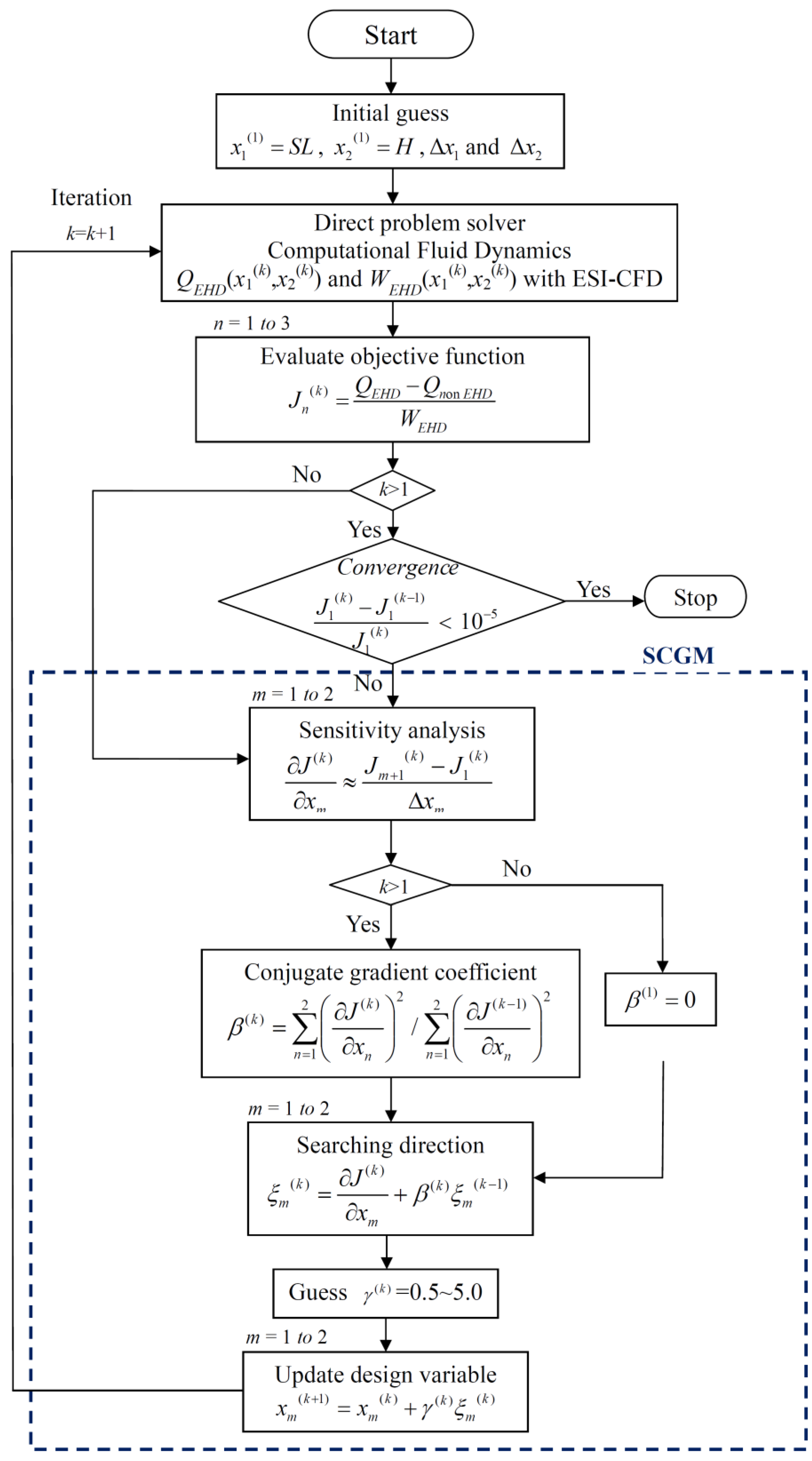
3.3. Optimization

In the current study, the objective functions J(x₁, x₂) were defined as the maximum heat transfer enhancement per unit power consumption (Nu_EHD − Nu_nonEHD)/W_EHD, as shown in Equation (23). The SCGM method was used to search the optimal electrode pitch (SL) and electrode height (H). The procedure were as follows:

• Guess the initial values for the two design variables (x₁, x₂), the electrode height (H), and the electrode pitch (SL).
• Utilize the finite difference method to solve for the velocity field (U), electric field strength (E), and temperature field (T), and the objective function J(x₁, x₂) associated with the new values of H and SL.
• When the obtained value of J(x₁, x₂) a maximum, the optimization search procedure is stopped. Otherwise, continue to Step 4.
• By increasing a small increment (Δx₁, Δx₂), the gradient functions (∂J/∂x₁)^(k) and (∂J/∂x₂)^(k) can be computed using the following algebraic manipulation:

  $$\frac{\partial J_1{}^{(k)}}{\partial x_1}\approx \frac{J_1{}^{(k)}-J^{(k)}}{\mathsf{\Delta }{x}_1}\mathrm{and}\frac{\partial J_2{}^{(k)}}{\partial x_2}\approx \frac{J_2{}^{(k)}-J^{(k)}}{\mathsf{\Delta }{x}_2},$$

  (23)
• The conjugate gradient coefficients β_c^(k) and the search directions ξ₁^{(k + 1)} and ξ₂^{(k + 1)} can be obtained as follows.

  $${\beta }_c{}^{(k)}=\frac{{\displaystyle \sum _{n=1}^2{\left(\frac{\partial J_n{}^{(k)}}{\partial x_n}\right)}^2}}{{\displaystyle \sum _{n=1}^2{\left(\frac{\partial J_n{}^{(k-1)}}{\partial x_n}\right)}^2}},\left(\mathrm{When}k=1,{\beta }_c{}^{(1)}=0\right)$$

  (24)

  $${\xi }_1{}^{(k)}={(\frac{\partial J}{\partial x_1})}^{(k)}+{\beta }_c{}^{(k)}{\xi }_1{}^{(k-1)}\mathrm{and}{\xi }_2{}^{(k)}={(\frac{\partial J}{\partial x_2})}^{(k)}+{\beta }_c{}^{(k)}{\xi }_2{}^{(k-1)},$$

  (25)
• The new update design variables is calculated as follows:

  $$x_1{}^{(k+1)}=x_1{}^{(k)}+\gamma {\xi }_1{}^{(k)}\mathrm{and}{x}_2{}^{(k+1)}=x_2{}^{(k)}+\gamma {\xi }_2{}^{(k)},$$

  (26)

The flowchart for the SCGM optimization process is shown in Figure 4.

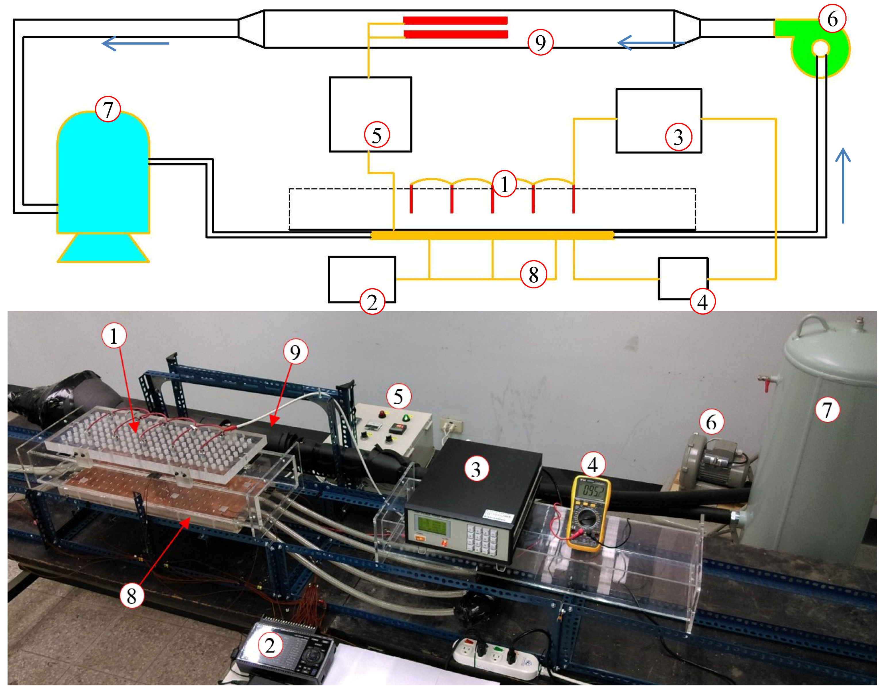
4. Experimental Facilities and Methods

The experimental setup is schematically illustrated in Figure 5. The room surroundings outside the test body are controlled at a constant temperature. The test facility includes an electrode structure, a heating cycle system, and a measured section.

4.1. Electrode Structure

In this experiment, multiple tungsten electrodes (ϕ 1.0 mm × 150 mm) were mounted into the framework. They were fixed to compress the collet with the screw on the specified holes. The height of the electrode was determined by the distance piece. The electrodes were connected in parallel and voltage was applied with a high-voltage power supply (YOU-SHANG SM4030-24PIR V₀ = 0–40 kV). The top of the needle electrode was applied as positive electricity, and the ground plate (isothermal heated plate) was considered to be negative electricity. A micro ammeter was connected between the ground plate and the high-voltage power supply to obtain the corona current.

4.2. Heating Cycle System

An isothermal heated plate was heated to create circular air heating. First, an air blower (DARGANG DG-200 11 0.5 kW single phase) and a heating controller (HAO-CHEN 110 V15 A) were turned on to lead air into the channel for heating. Two heaters (200 W/110 V) were placed in the middle of the tunnel to heat the air. The heated air entered the surge tank from the inlet to mix into the air in the tank, and the mixed air was output from the outlet. The hot air enters the test section via four insulated tubes. This test section (the isothermal heated plate) was heated from the surge tank to transport uniformly heated air. The air blower absorbed the exhausted air via four insulated tubes from the heated plate, and it was transported again to the channel for repeated heating. The heating cycle was repeated until the wall temperature was maintained at the prescribed value.

4.3. Measuring Section

A data recorder (GRAPHTEC midi LOGGER GL820) was set to capture the temperatures using fifteen K-type thermocouples with an accuracy of ±0.1 °C. They were mounted at the central test core (i.e., six on the heated plate, six under the heated plate, and three outside the framework). The temperatures of thermocouples were recorded and averaged. In terms of steady-state values, the random variation of these thermocouples was within ±0.1 °C. The high-voltage power supply had a maximum power limit of 30 W and a maximum output voltage of 40 kV. The accuracy of the power supply was ±2% for voltage. The corona currents were measured using a digital ammeter (HILA DM2650). Five ranges (20 A to 200 μA) were available depending on the experimental need. The accuracy was within ±0.5%. A thermocouple was installed on the heating wall to provide feedback on the heating temperature to the temperature controller. Using the method suggested by Kline and McClintock [21], the estimated uncertainty was 4.1% for the Nusselt number and 4.5% for the objective function E_b (net heat transfer benefit). The uncertainty was mainly due to the corona current measurement, especially at input voltages close to the threshold voltage. The uncertainties are tabulated in

Table 1. Summary of estimated uncertainties.

Primary Measurement		Derived Measurement
Parameter	Uncertainties	Parameter	Uncertainties
	V0 = 16 kV
V0	2%	Nu	4.1%
I	0.5%	Eb	4.5%
T∞	0.1 °C	-	-
Tw	0.1 °C	-	-

. To minimize the measurement precision uncertainty, the experiment was executed ten times under the same conditions, and then the average values were tabulated.

5. Results and Discussion

The research in this article was mainly focused on the optimization of the heat transfer enhancement per unit power consumption (E_b) obtained with the electro-hydraulic wind effect of needle electrodes. The heat transfer enhancement per unit power consumption was defined as the objective optimization function, and SCGM was used to search for the best combination of electrode height and pitch.

In order to avoid the danger of electric shock due to high applied voltage, constant temperature air circular heating instead of constant temperature water heating cycle was adopted as the experimental heating method. The electrodes were fixed to compress the collet with the screw on the framework. In order to ensure the accuracy of the electrode height (the distance between the electrode tip and the ground plate), distance pieces ranging in length from 20 to 60 mm at intervals of 10 mm were made. The operating parameters of the experiment included applied voltage and electrode arrangement (height and pitch). The applied voltage V₀ ranged from 8 kV to 40 kV and was executed at intervals of 1 kV until breakdown. The electrode height ranged from 20 mm to 60 mm and was executed at intervals of 10 mm with a fixed electrode pitch (SL = 100 mm). The electrode pitch ranged from 50 mm to 200 mm (SL = 50 mm, 75 mm, 100 mm, 150 mm, 200 mm) and was executed with a fixed electrode height (H = 30 mm). When the electrodes were mounted at the specified height and pitch, the power was applied from 8 kV and increased at intervals of 1 kV until breakdown. Each measured point had to be stable during the experimental procedure. The above steps were repeated to complete all the cases, and then the data were drawn as a V-I curve, as shown in Figure 6.

Figure 6 shows the experimental charge density for the electrode surface (ρ_c0) distributions versus electrode height (H) and electrode pitch (SL) for the specified applied voltages. The results show that the charge density of the electrode surface (ρ_c0) varied within 15% among the variations in electrode pitch (SL) as Figure 6a, but it varied 2.8 times to 7.9 times among the variations in electrode height (H) as Figure 6b. This finding is consistent with that of Leu et al. [19]. Therefore, the charge density can be assumed to be influenced predominantly by electrode height. In addition, the experimental data show that the quadratic relation is fit to be the relationship each other. This relation is also subsequently used in the optimization analysis. The quadratic relations are developed for the cases of specified applied voltage (V₀ = 12 kV, 14 kV, 16 kV, 18 kV, 20 kV) and temperature difference (ΔT = 33 K, 53 K, 73 K). The corresponding available ranges of electrode height (H) were 15 mm < H < 40 mm, 15 mm < H < 40 mm, 15 mm < H < 45 mm, 20 mm < H < 50 mm and 25 mm < H < 55 mm, respectively. The units of ρ_c0 and H were μC/m³ and mm.

Figure 7 shows the comparisons of Nusselt number ratio (Nu_EHD/Nu_nonEHD) between the numerical simulation and the experimental results versus electrode height for the specified voltages with respect to the model shown in Figure 6a. Nu_EHD/Nu_nonEHD represents the Nusselt number ratio of the cases with and without the EHD effect, which is used to interpret the EHD-induced heat transfer enhancement. The comparisons show good agreement, with a maximum discrepancy of 10.5%. This means the present numerical simulations have good accuracy for the studied topic.

Figure 8 shows the microscopic distribution of the flow field vector, and temperature at specified voltages (V₀ = 0 V, 12 kV and 20 kV) and electrode height (H = 25 mm) at ΔT = 53 K and SL = 150 mm. As shown in Figure 8a, it is a pure natural convection flow, where the flow field moves to the middle and top exterior. Figure 8b (V₀ = 12 kV) and Figure 8c (V₀ = 20 kV) show the flows with EHD, where the flows near the electrodes move downward to impinge against the bottom wall and then result in the vortex pairs between the electrodes regions. The flows in the left and right sides outflow to the exterior. The case of V₀ = 20 kV (Figure 8c) has a stronger vortex structure than that of V₀ = 12 kV (Figure 8b). Figure 8d is the case of pure natural convection, where the temperature distribution in the middle has a thick boundary layer that exhibits less heat transfer. Figure 8e,f are the cases with EHD. The regions near the electrodes have a thinner boundary layer, so there is better heat transfer performance. Furthermore, the case of Figure 8f with V₀ = 20 kV is better than the case of V₀ = 12 kV. Figure 9 shows the variations in the local Nusselt number (Nu_{EHD_x}) along the x-direction for the five electrode heights (H = 20, 25, 30, 35 and 40 mm) at ΔT = 53 K, V₀ = 16 kV, and SL = 100 mm. It clearly indicates that Nu_{EHD_x} increases with decreases in the electrode height and is significantly larger at the electrode locations.

Figure 10 illustrates the variations in the Nu_EHD/Nu_nonEHD versus electrode height H for V₀ = 12, 14, 16, 18, and 20 kV at SL = 150 mm and ΔT = 53 K. The value of Nu_EHD/Nu_nonEHD increases with increases in the applied voltage or decreases in the electrode height. In addition, the maximum values of Nu_EHD/Nu_nonEHD for V₀ = 12, 14, 16, 18, and 20 kV are 1.29, 1.51, 1.70, 1.86 and 1.88, respectively. Figure 11 illustrates the variations in the Nu_EHD/Nu_nonEHD versus electrode pitch SL for V₀ = 12, 14, 16, 18, and 20 kV at H = 25 mm and ΔT = 53 K. The values of Nu_EHD/Nu_nonEHD increased with increases in the applied voltage, and the maximum value for the specified V₀ is obtained. The maximum values of Nu_EHD/Nu_nonEHD for V₀ = 12, 14, 16, 18, and 20 kV are 1.16, 1.39, 1.62, 1.79 and 1.95, respectively. Figure 10 and Figure 11 indicate that the electrode height and pitch effectively enhance the heat transfer performance. Figure 12 illustrates the variations in the Nu_EHD/Nu_nonEHD versus ΔT for specified applied voltages V₀ = 12, 14, 16, 18, and 20 kV at H = 25 mm and SL = 150 mm. The figure shows that the values of Nu_EHD/Nu_nonEHD increase with increases in applied voltage but decrease with increases in the temperature difference. The reason for this is that a larger temperature difference means a more violent natural convection flow, while the EHD-induced flow is weaker relative to the main flow.

A more realistic EHD heat transfer enhancement criteria, E_b (E_b = (Nu_EHD − Nu_nonEHD)/W_EHD), is proposed to evaluate EHD-enhanced heat transfer per power consumption. Figure 13 illustrates the variations in the E_b versus applied voltage V₀ for H = 20, 25, 30, 35, and 40 mm at SL = 150 mm and ΔT = 53 K. The difference in E_b value decrease with increases in applied voltage, and the effect in electrode height decrease with increase in applied voltage. In addition, the maximum values of E_b for H = 20, 25, 30, 35, and 40 mm are 6.31, 6.02, 5.58, 5.09 and 4.67, respectively. Figure 14 illustrates the variations in the E_b versus applied voltage V₀ for SL = 50, 75, 100, 125, 150, 175 and 200 mm at H = 25 mm and ΔT = 53 K. The difference in E_b value decrease with increases in applied voltage, and the effect in electrode pitch decrease with increase in applied voltage. The maximum values of E_b for SL = 50, 75, 100, 125, 150, 175 and 200 mm are 3.45, 4.77, 5.95, 7.24, 6.02, 3.25 and 3.03, respectively. Figure 13 and Figure 14 indicate that the electrode height and pitch in appropriate arrangement effectively enhance the heat transfer enhancement per power consumption, and this means that the smaller electrode height and the intensive electrode pitch do not give better benefit. Therefore, the appropriate electrode pitch and height reveal the better benefit on both efficiency and economics. Figure 15 illustrates the variations in the E_b versus applied voltages V₀ for ΔT = 33, 53, and 73 K at H = 25 mm and SL = 150 mm. The variation in E_b value decrease with increases in the temperature difference. The maximum values of E_b for ΔT = 33, 53, and 73 K are 7.90, 6.02 and 4.76. Figure 16 shows the variations in E_b for SL ranging from 50 to 200 mm at ΔT = 53 K and V₀ = 16 kV where the specified electrode height H was H = 15, 20, 25, 30, 35, 40 and 45 mm. The results indicate the maximum E_b values were 5.26, 5.60, 5.72, 5.58, 5.20, 4.55, and 3.52 for specified values of H, respectively. In conclusion, the maximum E_b occurred at H = 25 mm and SL = 150 mm. It is worth mentioning that the negative values of E_b occurred at SL = 50 mm and SL = 200 mm for the cases of H = 40 mm and 45 mm. This means the EHD effect now is a penalty for heat transfer enhancement. In fact, an unsuitable electrode system really induces a worse heat transfer scheme as the “EHD-induced barrier effect” described in Wang et al. [22].

Figure 17a–c display the iteration process used to search for the optimum electrode height (H) and pitch (SL) combination for the maximization of objective function (i.e., heat transfer enhancement per power consumption, E_b) at V₀ = 16 kV, with (a) ΔT = 33 K, (b) ΔT = 53 K and (c) ΔT = 73 K, respectively. The contours of the net heat transfer benefit are plotted as a function of H and SL, where the dark red area represents the maximum heat transfer enhancement per power consumption. It can be seen that, by using the simple conjugated gradient method (SCGM), the optimal H and SL combination are obtained (H = 32.2 mm and SL = 125.8 mm), (H = 27.5 mm and SL = 128.2 mm), and (H = 28.3 mm and SL = 125.9 mm) for 14, 13, and 8 iterations, respectively, with the initial value of H_i = 15 mm and SL_i = 50 mm. The heat transfer enhancement per unit power consumption are 7.96, 6.36, and 5.50, respectively. In conclusion, the optimization method provides a tremendous savings in regard to computational time for the studied topic. The obtained optimal combinations of H and SL for specified V₀ (V₀ = 12, 14, 16, 18, and 20 kV) and ΔT (ΔT = 33, 53 and 73 K) are tabulated in

Table 2. The searched optimum combination of H and SL for different applied voltages V₀ and temperature differences ΔT.

V0 (kV)	H (mm)	SL (mm)	Eb (1/W)	Iteration No.
(a) ΔT = 33 K	-	-	-	-
12	17.7	127.0	9.72	15
14	24.2	126.5	8.78	19
16	32.2	125.8	7.96	14
18	38.2	125.9	7.19	15
20	45.6	129.4	6.41	19
(b) ΔT = 53 K	-	-	-	-
12	19.3	126.9	7.81	14
14	22.6	126.7	7.08	23
16	27.5	128.2	6.36	13
18	33.8	128.2	5.79	16
20	37.4	127.2	5.26	12
(c) ΔT = 73 K	-	-	-	-
12	16.8	123.1	6.39	16
14	17.6	130.6	7.77	12
16	28.3	125.9	5.50	8
18	29.5	128.6	4.92	17
20	34.1	130.9	4.42	21

.

Table 2 shows that, for a given temperature difference (ΔT) between the wall and ambient, the optimal electrode height increases with increase in the applied voltage. This is due to the fact that, as the electrode height is increased, the corona current and also the power consumption are decreased. In addition, for a given applied voltage, the optimal electrode height decreases with increasing temperature difference (ΔT). This is because EHD heat transfer enhancement becomes stronger when the degree of natural convection (ΔT) is decreased. Then, for a specified applied voltage, the lower electrode height results in higher heat transfer enhancement per unit power consumption (E_b). As for the location of optimal electrode pitch, the variation of optimal electrode pitch is insignificant with the variations of applied voltage and temperature difference. It is because the power consumption is less affected by the variation of electrode pitch.

6. Conclusions

The main purpose of this study was to use the ion wind generated by needle electrodes to impinge a wall temperature and enhance heat transfer. The fluid flow was assumed to be three-dimensional, steady and turbulent. The heat transfer enhancement per the input power was defined for the heat transfer enhancement per power consumption (E_b), which involved maximizing the objective function to search for the optimum electrode pitch (SL) and electrode height (H) combination. We can draw the following conclusions:

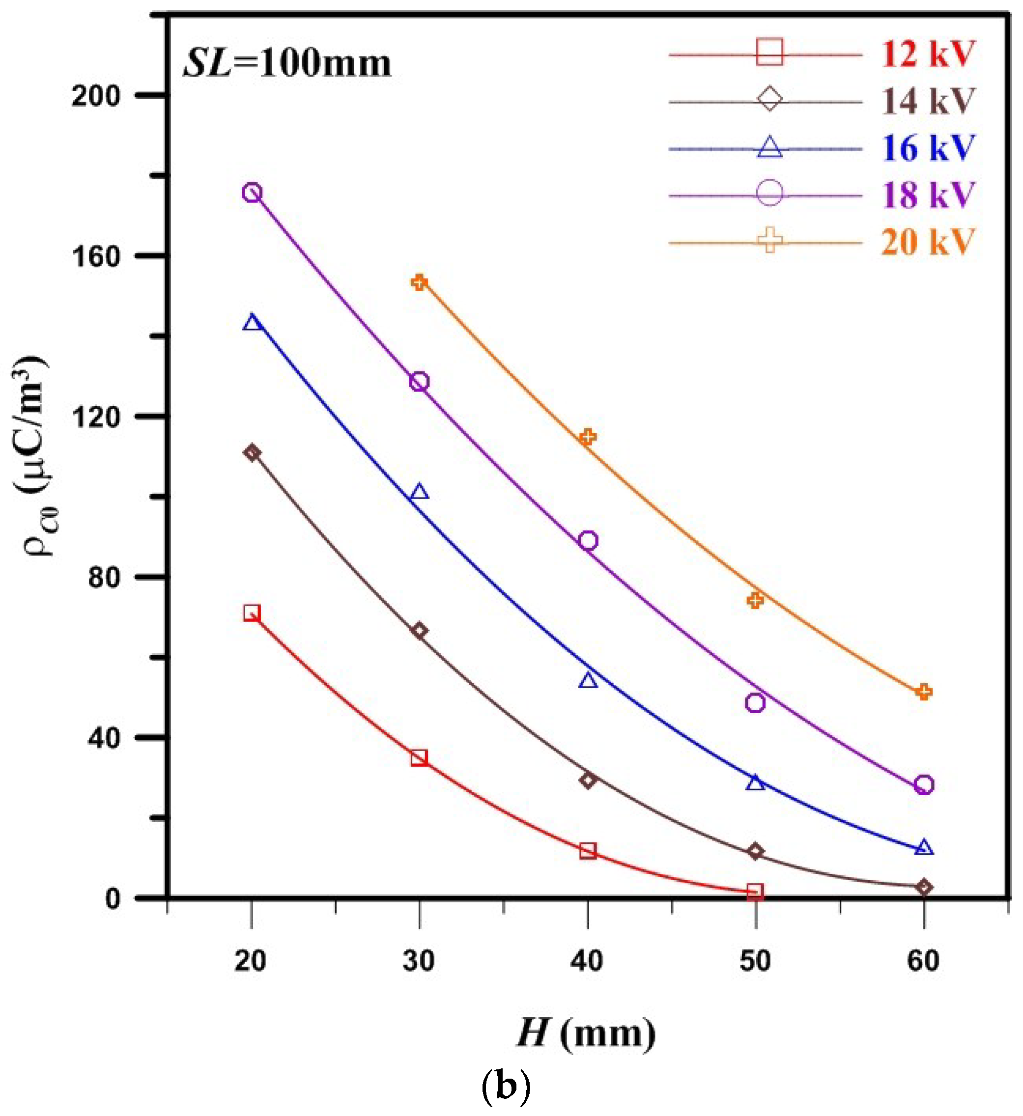
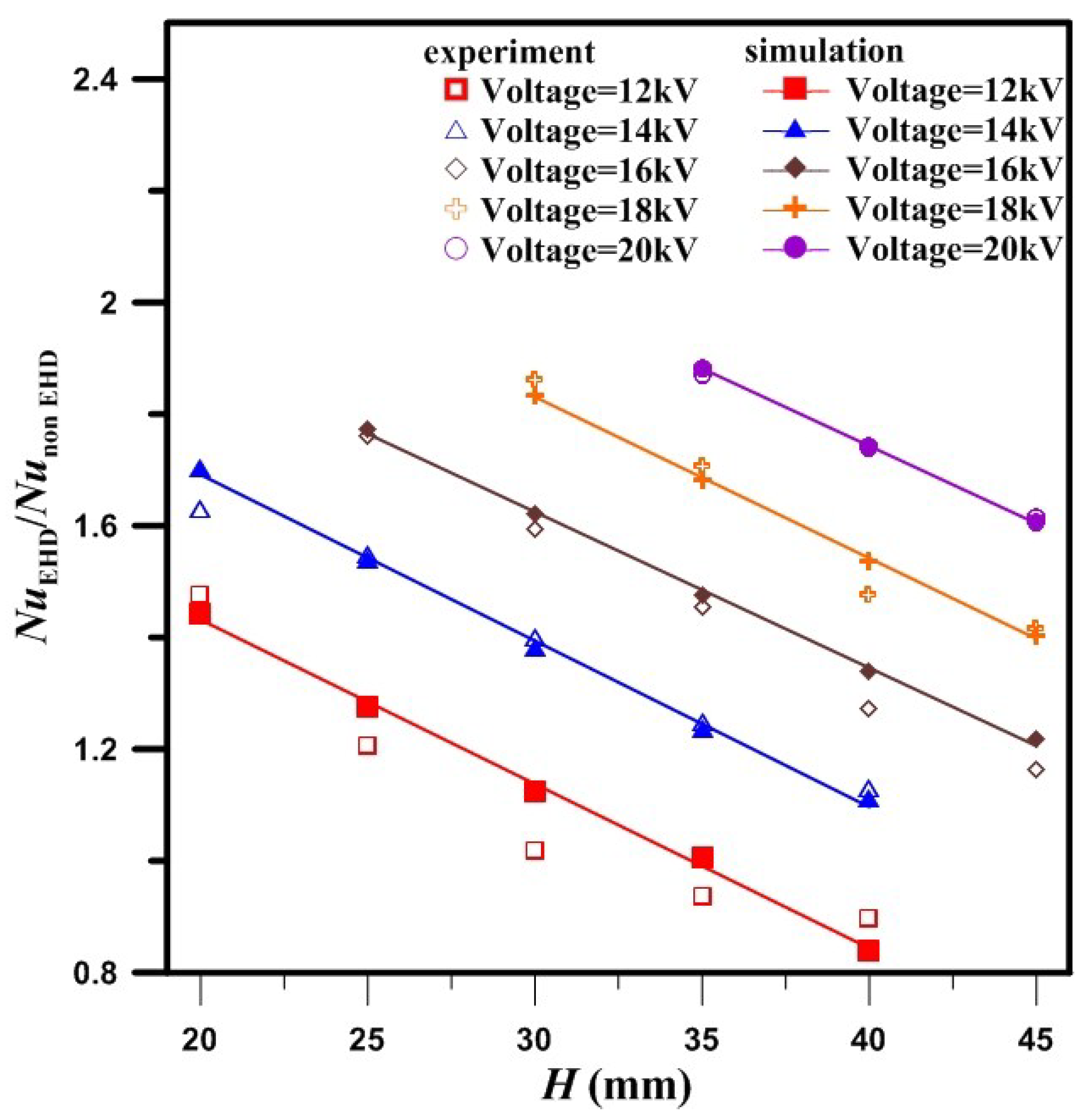
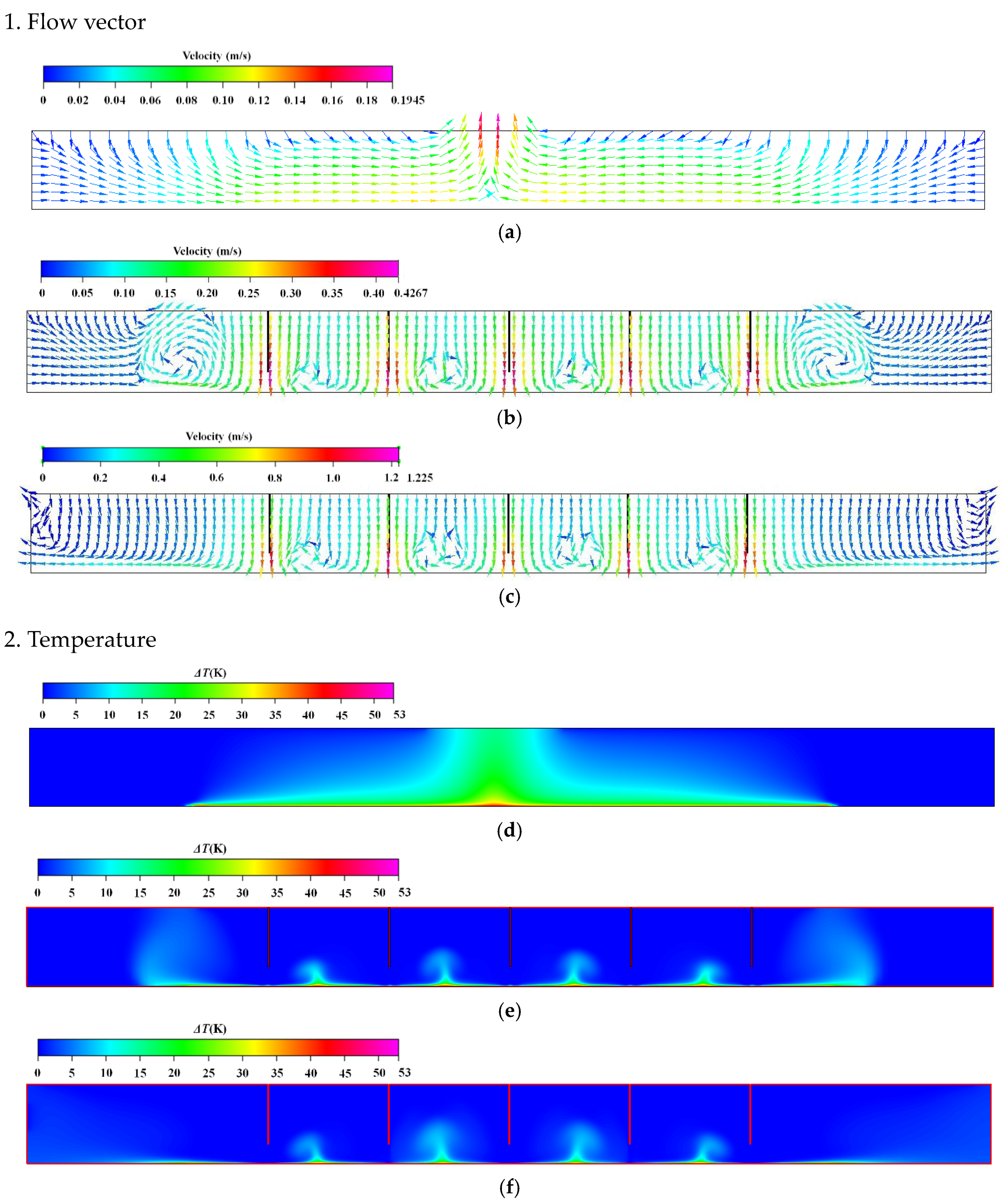
• The ion-wind effect caused by EHD actually disrupted the flow and enhanced the mixing of the fluids. Therefore, EHD technology can effectively improve heat transfer performance. The heat transfer was increased with increases in the applied voltage.
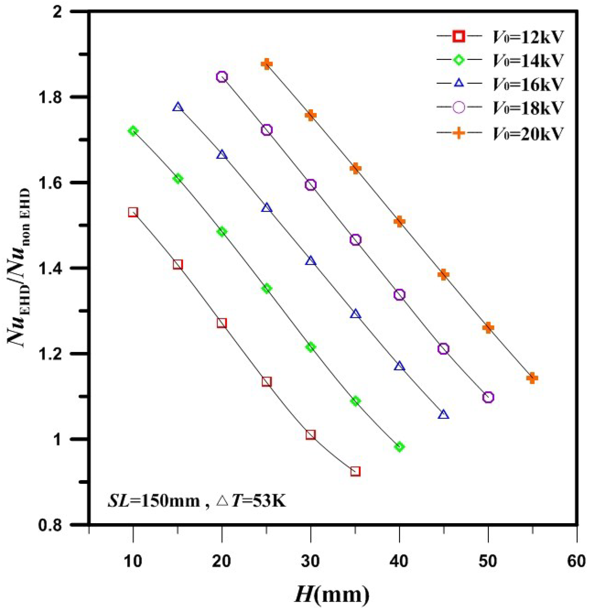
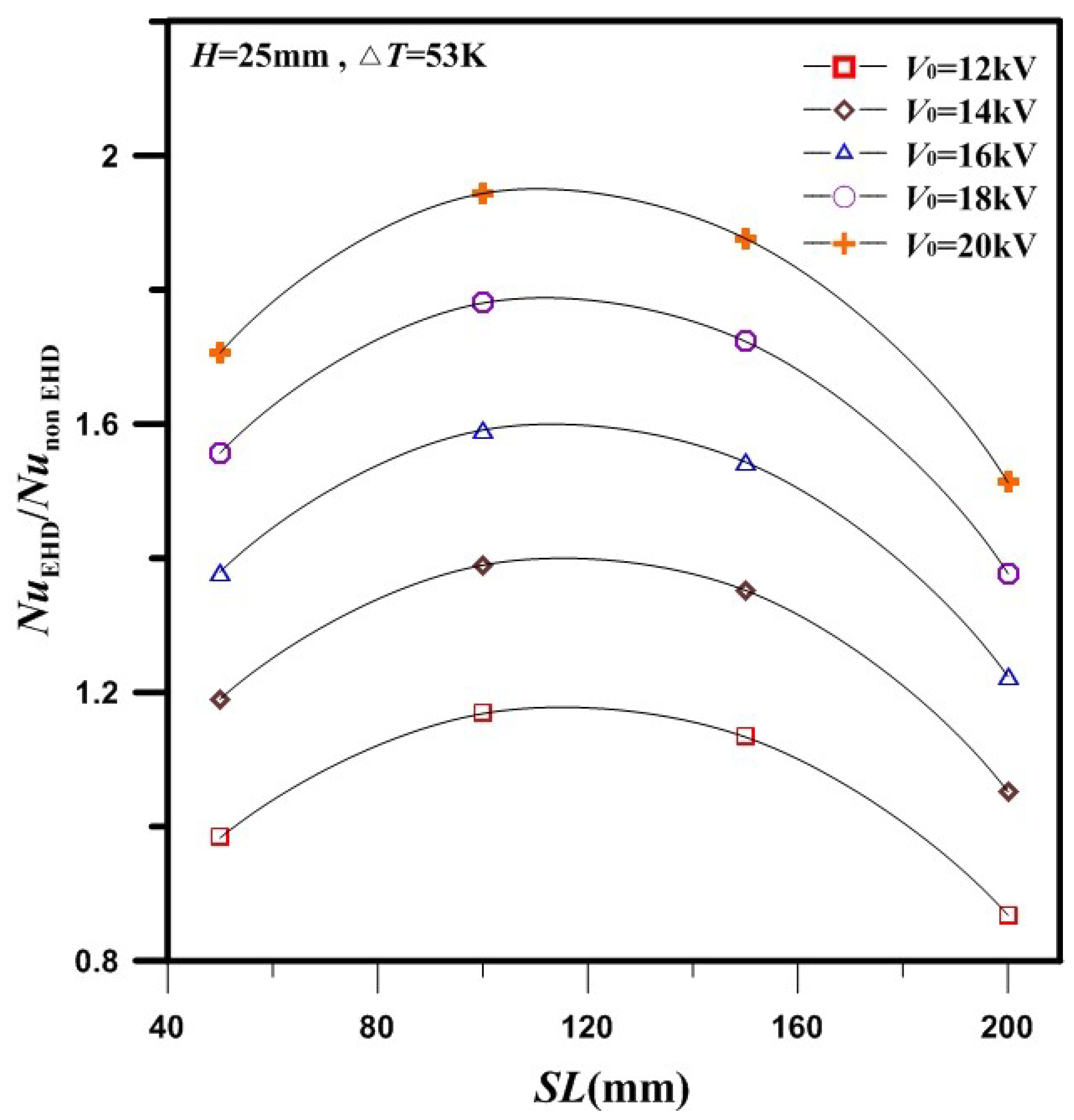
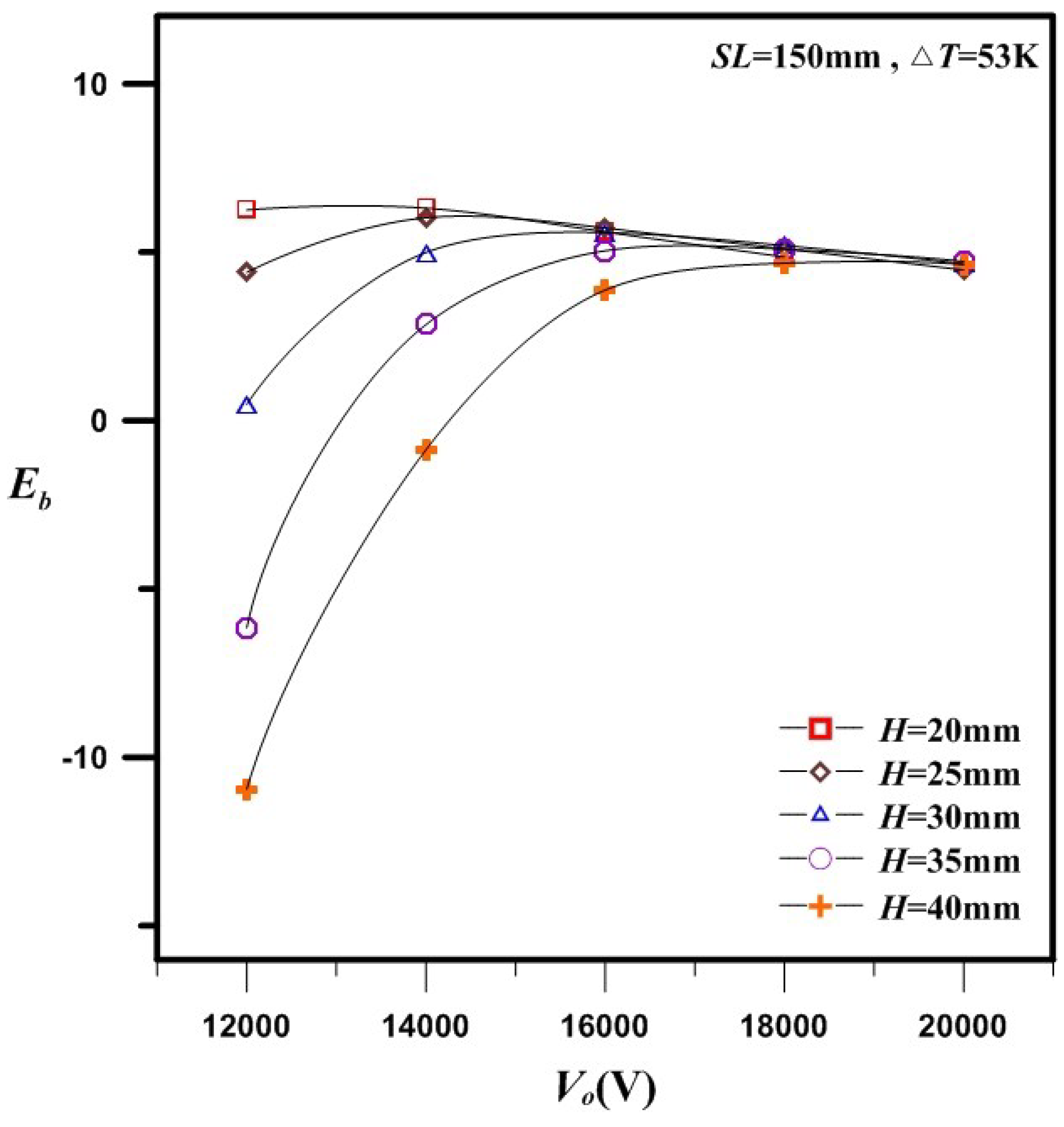
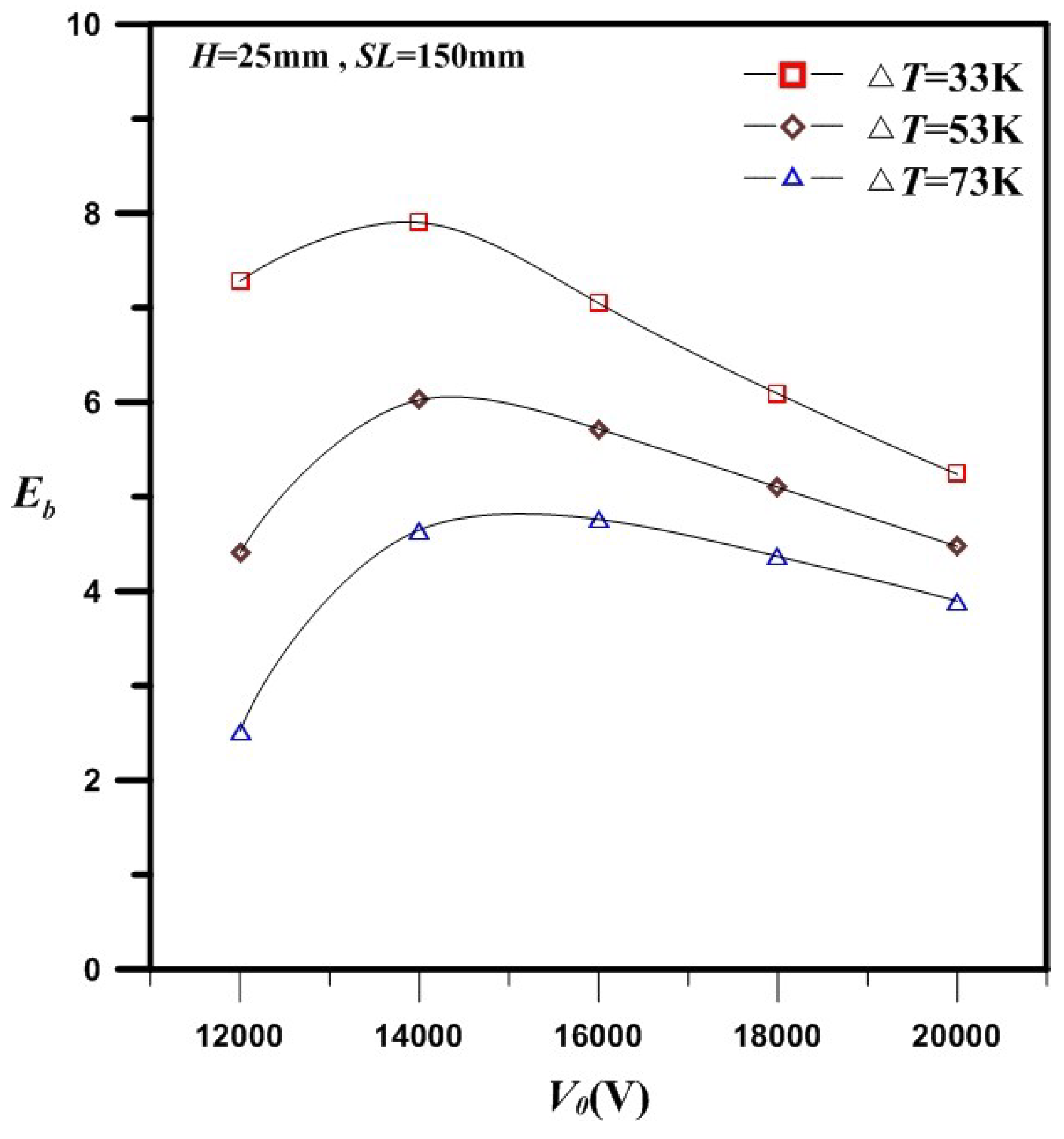
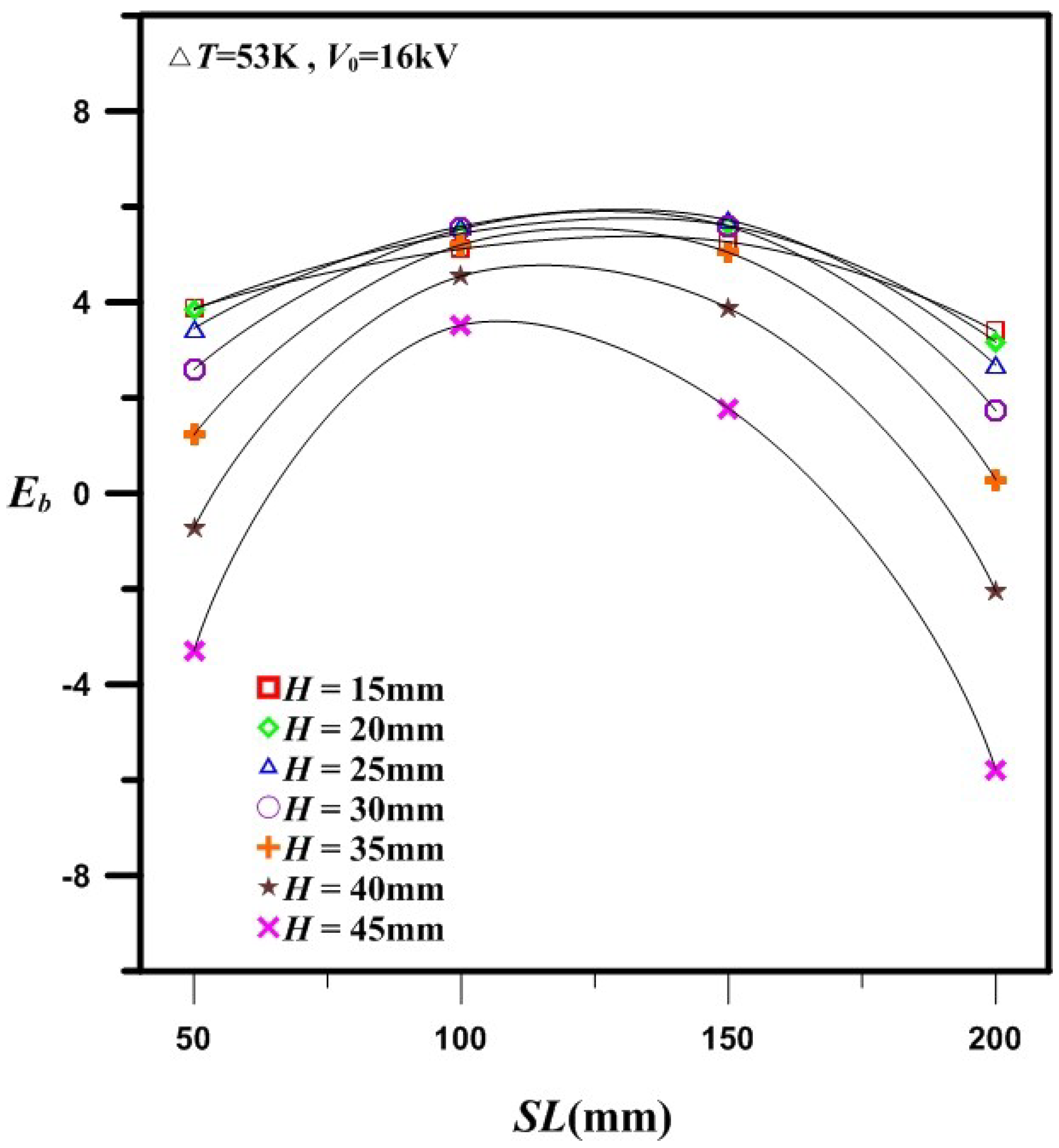
• The smaller electrode height and the intensive electrode pitch do not give better the heat transfer enhancement per power consumption E_b. The appropriate electrode pitch and height reveal the better benefit on both efficiency and economics. Therefore, the study obtained the optimal combinations of H and SL for specified V₀ (V₀ = 12, 14, 16, 18, and 20 kV) and ΔT (ΔT = 33, 53 and 73 K) and tabulated in Table 2.
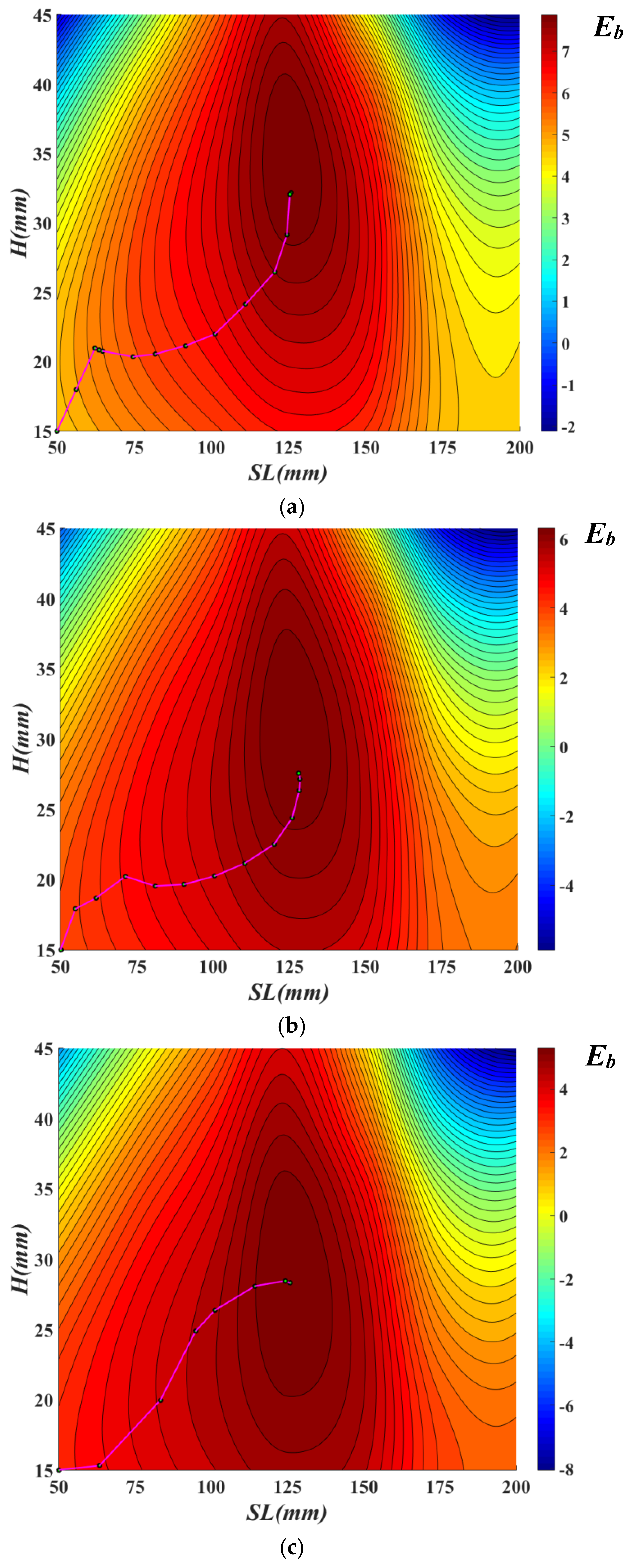
• In the optimization search process with V₀ = 12 kV and ΔT = 33 K using SCGM, the maximum value of heat transfer enhancement per power consumption was obtained at the 15th iteration. In addition, using a parametric analysis, the maximum value was obtained at the 806th iteration (15 mm < H < 40 mm take 26 nodes and 50 mm < SL < 200 mm take 31 nodes). Therefore, SCGM is much faster than a parametric analysis.

References

- Marco, S.M.; Velkoff, H.R. Effect of Electrostatic Fields on Free Convection Heat Transfer from Flat Plate. ASME J. Heat Transf. 1963, 63, 9. [Google Scholar]
- O’brien, R.; Shine, A. Some effects of an electric field on heat transfer from a vertical plate in free convection. ASME J. Heat Transf. 1967, 89, 114–116. [Google Scholar] [CrossRef]
- Kibler, K.; Carter, H. Electrocooling in gases. J. Appl. Phys. 1974, 45, 4436–4440. [Google Scholar] [CrossRef]
- Franke, M.; Hogue, L. Electrostatic cooling of a horizontal cylinder. ASME Trans. J. Heat Transf. 1991, 113, 544–548. [Google Scholar] [CrossRef]
- Owsenek, B.L.; Seyed-Yagoobi, J.; Page, R.H. Experimental investigation of corona wind heat transfer enhancement with a heated horizontal flat plate. J. Heat Transf. 1995, 117, 309–315. [Google Scholar] [CrossRef]
- Owsenek, B.L.; Seyed-Yagoobi, J. Theoretical and experimental study of electrohydrodynamic heat transfer enhancement through wire-plate corona discharge. J. Heat Transf. 1997, 119, 604–610. [Google Scholar] [CrossRef]
- Bhattacharyya, S.; Peterson, A. Corona Wind-Augmented Natural Convection-part 1: Single Electrode Studies. J. Enhanc. Heat Transf. 2002, 9, 209–219. [Google Scholar] [CrossRef]
- Huang, R.T.; Sheu, W.J.; Wang, C.C. Heat transfer enhancement by needle-arrayed electrodes—An EHD integrated cooling system. Energy Convers. Manag. 2009, 50, 1789–1796. [Google Scholar] [CrossRef]
- Go, D.B.; Garimella, S.V. Fisher, T.S.; Mongia, R.K. Ionic winds for locally enhanced cooling. J. Appl. Phys. 2007, 102, 053302. [Google Scholar] [CrossRef]
- Jewell-Larsen, E.N.; Ran, H.; Zhang, Y.; Schwiebert, M.K.; Honer Tessera, K.A. Electrohydrodynamic (EHD) cooled laptop. In Proceedings of the IEEE 25th SEMI-THERM, San Jose, CA, USA, 15–19 March 2009; pp. 261–266. [Google Scholar]
- Shakouri, P.M.; Esmaeilzadeh, E. Experimental investigation of convective heat transfer enhancement from 3D-shape heat sources by EHD actuator in duct flow. Exp. Therm. Fluid Sci. 2011, 35, 1383–1391. [Google Scholar] [CrossRef]
- Peng, M.; Wang, T.H.; Wang, X.D. Effect of longitudinal electrode arrangement on EHD-induced heat transfer enhancement in a rectangular channel. Int. J. Heat Mass Transf. 2016, 93, 1072–1081. [Google Scholar] [CrossRef]
- Heidarinejad, G.; Babaei, R. Numerical investigation of electro hydrodynamics (EHD) enhanced water evaporation using Large Eddy Simulation turbulent model. J. Electrost. 2015, 77, 76–87. [Google Scholar] [CrossRef]
- Leu, J.S.; Jang, J.Y.; Wu, Y.-H. Optimization of the wire electrode height and pitch for 3-D electrohydrodynamic enhanced water evaporation. Int. J. Heat Mass Transf. 2018, 118, 976–988. [Google Scholar] [CrossRef]
- Lai, F.C.; Sharma, R.K. EHD-enhanced drying with multiple needle electrode. J. Electrost. 2005, 63, 223–237. [Google Scholar] [CrossRef]
- Lin, C.W.; Jang, J.Y. 3D Numerical heat transfer and fluid flow analysis in plate-fin and tube heat exchangers with electrohydrodynamic enhancement. Heat Mass Transf. 2005, 41, 583–593. [Google Scholar] [CrossRef]
- CFD-ACE(U); CFD Research Corporation: Huntsville, AL, USA, 2013.
- Quarteroni, A.; Sacco, R.; Saleri, F. Numerical Mathematics; Springer: New York, NY, USA, 2007. [Google Scholar]
- Launder, B.E.; Spalding, D.B. The Numerical Computation of Turbulent Flows. Comput. Methods Appl. Mech. Eng. 1974, 3, 269–289. [Google Scholar] [CrossRef]
- Liakopoulos, A. Explicit representation of the complete velocity profile in a turbulent boundary layer. AIAA J. 1984, 22, 844–846. [Google Scholar] [CrossRef]
- Kline, S.J.; McClintock, F.A. Describing uncertainties single-sample experiments. ASME Mech. Eng. 1953, 75, 3–8. [Google Scholar]
- Wang, T.H.; Peng, M.; Wang, X.D.; Yan, W.M. Investigation of heat transfer enhancement by electrohydrodynamics in a double-wall-heated channel. Int. J. Heat Mass Transf. 2017, 113, 373–383. [Google Scholar] [CrossRef]