A Thermal Probability Density–Based Method to Detect the Internal Defects of Power Cable Joints

Abstract

Internal defects inside power cable joints due to unqualified construction is the main issue of power cable failures, hence in this paper a method based on thermal probability density function to detect the internal defects of power cable joints is presented. First, the model to calculate the thermal distribution of power cable joints is set up and the thermal distribution is calculated. Then a thermal probability density (TPD)-based method that gives the statistics of isothermal points is presented. The TPD characteristics of normal power cable joints and those with internal defects, including insulation eccentricity and unqualified connection of conductors, are analyzed. The results indicate that TPD differs with the internal state of cable joints. Finally, experiments were conducted in which surface thermal distribution was measured by FLIR SC7000, and the corresponding TPDs are discussed.

1. Introduction

Unqualified construction and external destruction are the main issues in internal defects of power cable joints. The statistics show that more than 70% of defects occurred in cable joints during the past decade [1]. Internal defects of power cables will cause an increase of electromagnetic loss, insulation aging, and surface temperature changes. Excessive contact resistance due to unqualified connections of conductors and eccentricity of the core are common internal defects of cable joints.

At present, many researchers concentrate on calculating and measuring power cable temperature characteristics, because the working conditions of cable joints can be derived from the surface temperature. Many measuring techniques have been proposed, including temperature sensors, optical fibers, infrared thermal imagers, and so on [2,3,4]. Due to the advantages of their noncontact, secure, and real-time characteristics [5,6], infrared thermal imagers are widely used in fault monitoring and diagnosing [7,8].

At present, researchers concentrate on thermal analysis to check the faults and ampacity of power cables. In [9], a method to invert the temperature of conductors in cable joints was proposed, which was composed of two parts, radial-direction temperature inversion (RDTI) in the cable and axial-direction temperature inversion (ADTI) in the conductor. Reference [10] stated that the failure of cables and their joints can be classified by estimating or measuring ambient temperature and other parameters, because the temperature of cable insulation is a function of both ambient temperature and thermal resistivity of the ground. Reference [11] applied thermographic analysis to analyze associated regions with high surface temperature and proposed a method to diagnose faulty connections of parallel conductors. In [12], an equivalent Laplace thermal model of single-core cable was developed with lumped parameter methods based on the thermal circuit model. Reference [13] found that the partial discharge activity of power cables can be used to reflect the temperature cycling caused by load variation. Insulation eccentricity and unqualified connections of conductors are common internal defects of cable. Insulation eccentricity of cable causes not only a huge waste of the material but also electrical property problems [14]. Excess contact resistance due to unqualified connection of conductors is the main contributor to overheating and can accelerate insulation aging [15,16]. At present, the common methods to evaluate the degree of insulation eccentricity are x-ray, photoelectromagnetic, and eddy current [17,18].

Based on current research, this paper presents a new method to detect internal defects of cable joints by using thermal probability density (TPD). First, a three-dimensional (3D) electromagnetic-thermal coupling model of power cable is established and thermal distribution is calculated. Then, the distributions of TPD under different insulation eccentricity conditions are analyzed. According to the characteristics of TPD, the insulation eccentricity of power cable joints can be judged accurately. A platform is built to verify the accuracy of the proposed method. Finally, applying this method to excess contact resistance, the contact coefficient K can also be determined.

2. Model for Thermal Distribution of Power Cable Joints

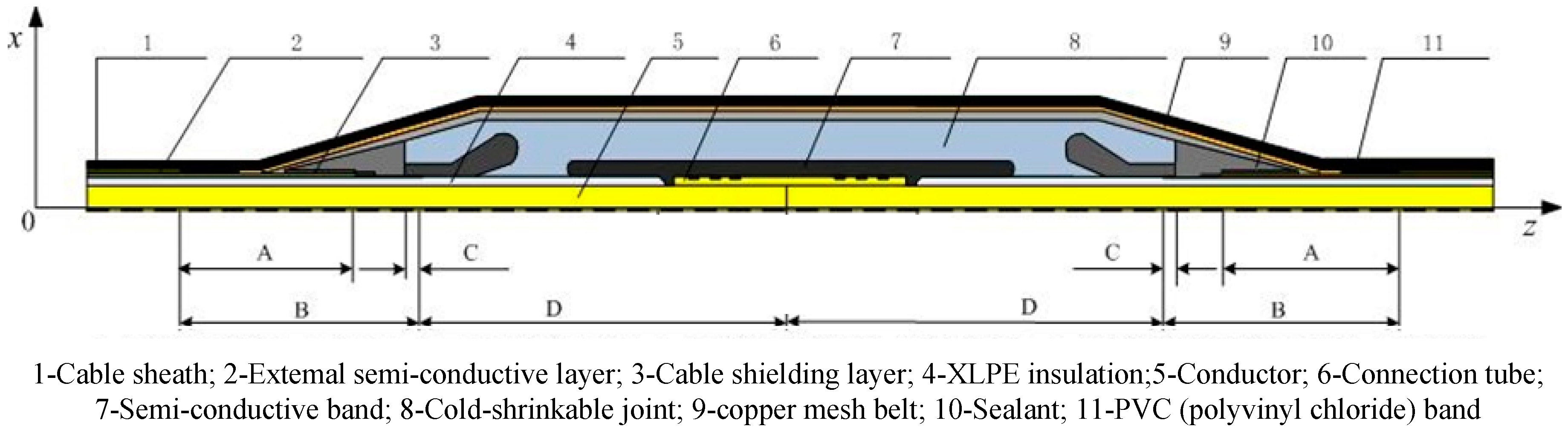
The XLPE (crosslinked polyethylene) power cable (8.7/15 kV YJV 1 × 400) is taken as an example, and an axial cross-section model of the cable joint is shown in Figure 1.

The parameters of the cable joint are shown in

Table 1. Parameters of cable joint.

Conductor diameter	23.8 mm
Insulation thickness	4.5 mm
Shielding layer thickness	0.5 mm
Sheath thickness	2.5 mm
External diameter of cable	41 mm
Conductor cross-section area	400 mm2

.

The lengths of different parts of the cable joint (as shown in Figure 1) are listed in

Table 2. Length parameters of cable joint (mm).

A	B	C	D	E
90	140	25	175	120

.

The parameters required for calculation in the temperature field are shown in

Table 3. Material physical parameters used for temperature field calculation.

Material	Thermal Conductivity/(W·(m·°C)−1)	Density/(kg·m−3)	Specific Heat Capacity/(J·(kg·°C)−1)
Conductor	400	8920	385
Semiconductor	0.48	1350	1470
Insulation	0.286	1200	2250
Sheath	0.167	1380	2100

.

For a single cable joint laid in the air, the laying parameters are given in

Table 4. Simulation parameters.

Ambient Temperature	Convection Heat Transfer Coefficient h	Current
20 °C	5.6 W/(m2·K)	1000 A

.

3. Thermal Probability Density Distribution–Based Method

Let T_max and T_min represent the maximum and minimum temperature, respectively. C_i is the count of T_i, where T_min < T_i < T_max.

Set $C_T={\displaystyle \sum C_i}$, P_i = C_i/C_T, which is known. $0\le P_i<1$, and ${\displaystyle \sum P_i=1}$.

It is obvious that when faults arise in high-voltage equipment, the thermal distribution changes, hence the curve of P_i will change, which can be used to determine internal faults. This is the thermal probability density (TPD)–based method.

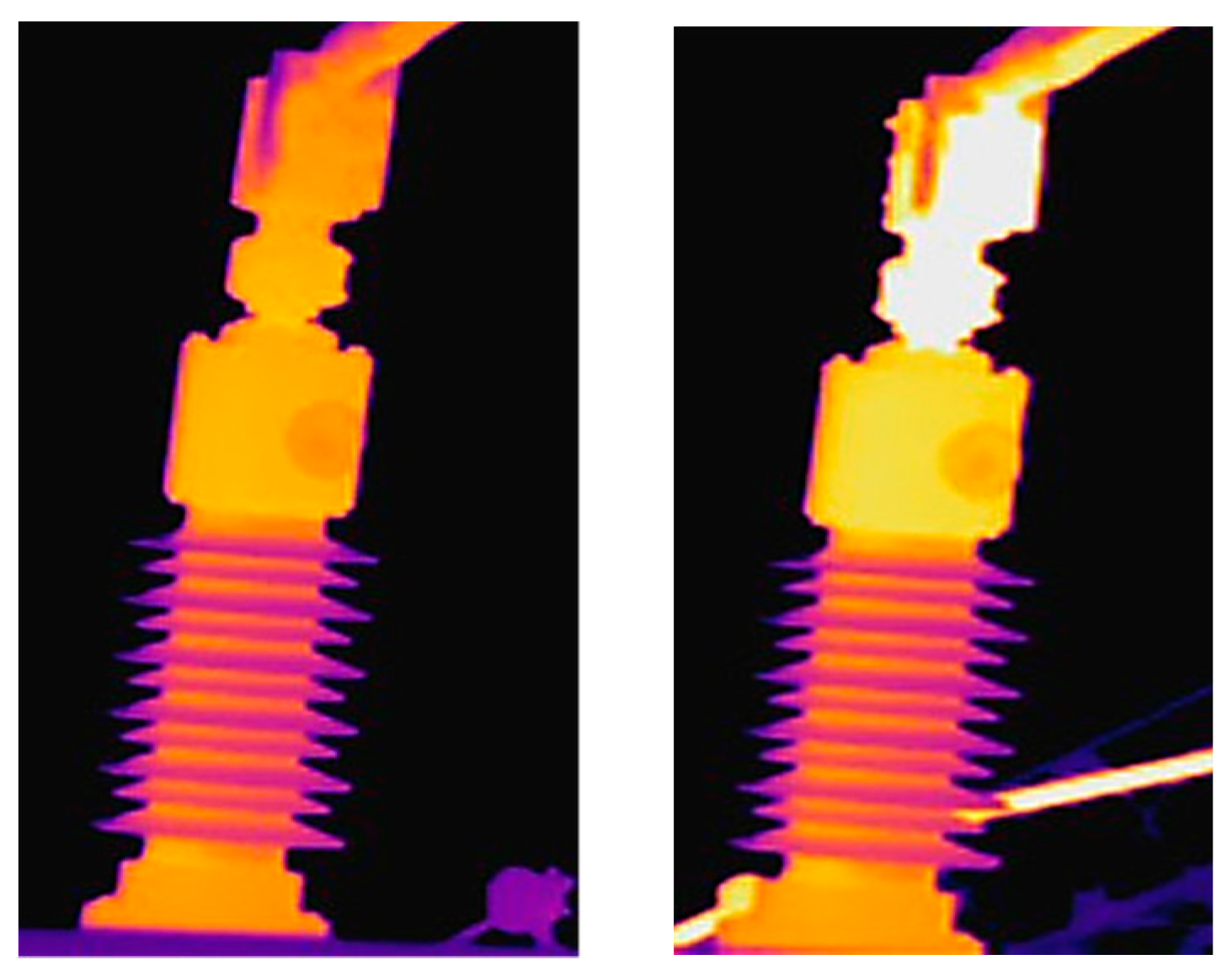
To use the TPD method in practice, infrared imaging technology can be used, which is widely used to analyze the operating state of electrical equipment and the contamination level of insulators. Two infrared images of low-voltage bushing under normal and fault conditions are shown in Figure 2.

The surface temperature distribution and the temperature span (the difference between T_max and T_min) will change with the operating conditions [19]. From the perspective of thermodynamic entropy, regarding each set of temperature data in the infrared image as a state, an infrared image contains a lot of temperature data, and a statistical method is chosen to analyze the data.

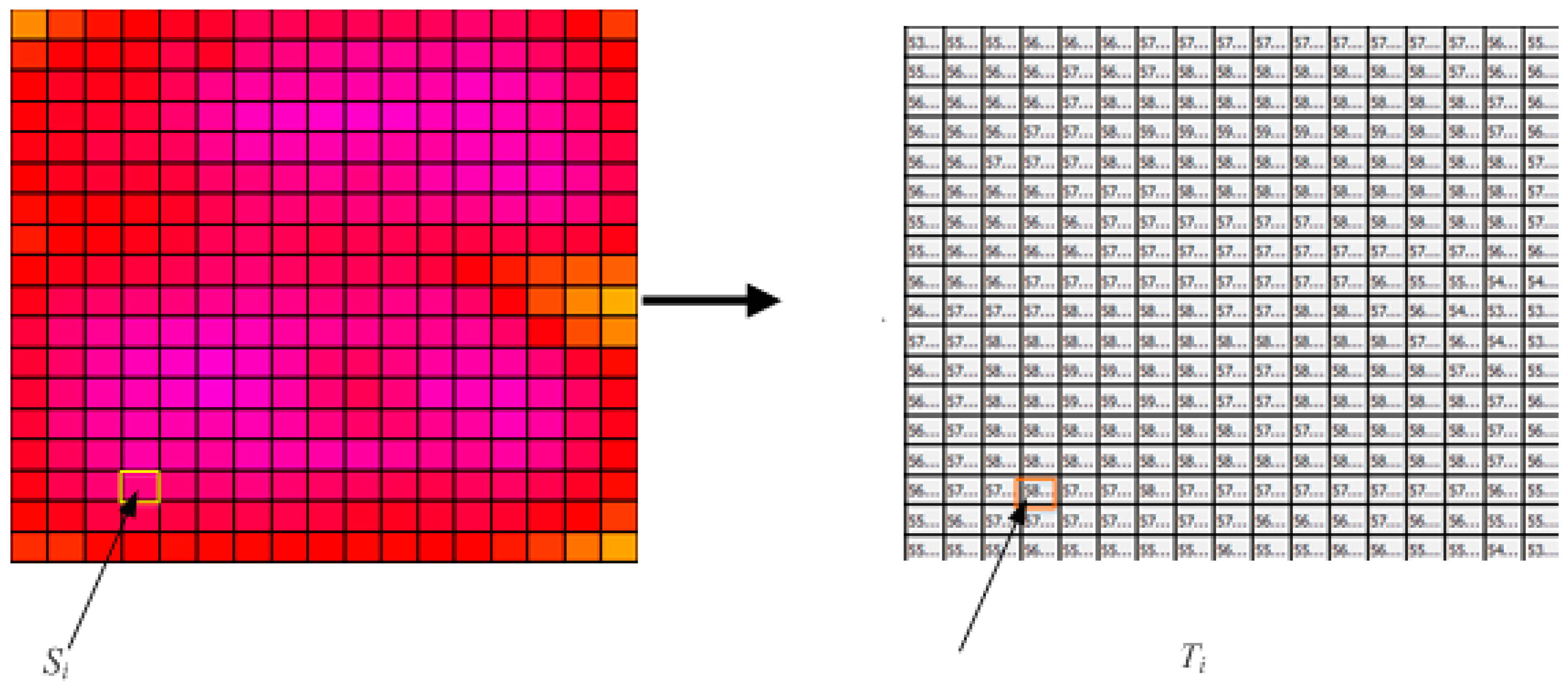
Probability density functions are often used to represent the distribution of data samples. As the cable surface temperature distribution is unknown, the nonparametric kernel density estimation method is used to calculate the surface temperature distribution [20,21]. The gray scale is used in infrared images to record the temperature data. Scattering the infrared image and treating temperature as a discontinuous physical quantity, the temperature matrix can be obtained, as shown in Figure 3. There are N × M temperature values in Figure 3, and each temperature value corresponds to a temperature state.

Dividing the entire temperature range into several small subintervals and regarding the temperatures located in the same subinterval as isothermal points T_i (T_min < T_i < T_max), the quantity of T_i can be determined using the statistical method, and then TPD can be drawn. The probability density of any temperature T_i is calculated according to Equation (1):

$$\widehat{y}\left(x\right)=\frac{1}{nh}{\displaystyle \sum }_{j=1}^{n}K\left(\frac{x-x_i}{h}\right)$$

(1)

where K(u) is a kernel function and h is the window width.

In order to verify the accuracy of the calculation results, the asymptotic mean integrated square error (AMISE) is often used to detect the accuracy of $\widehat{y}\left(x\right)$. The expression is as follows:

$$AMISE(h)=\frac{1}{nh}R(K)+\frac{1}{4}{h}^4{[{\mu }_2(K)]}^{2}R(y^{″})$$

(2)

where $R(K)={\displaystyle \int K{(z)}^{2}dz}$, ${\mu }_2(K)={\displaystyle \int z^{2}K(z)dz}$, $R(y^{″})={\displaystyle \int {[y^{″}(x)]}^{2}dz}$.

When $\frac{d}{dh}[AMISE(h)]=0$, the best window width value (h_optimal) can be calculated using Equation (3):

$$h_{optimal}={\{\frac{R(K)}{{[{\mu }_2(K)]}^{2}R(y^{″})n}\}}^{\frac{1}{5}}$$

(3)

The calculation results of h_optimal and AMISE under different kernel functions are shown in

Table 5. Results of several kernel functions. AMISE, asymptotic mean integrated square error.

Parameter	Uniform Kernel	Triangular Kernel	Gaussian Kernel
hoptimal	0.436806	0.618528	0.5548
AMISE (10−5)	7.7542	6.1584	5.7456

. The comparison results show that the Gaussian kernel function has the smallest error. The Gaussian kernel is shown in Equation (4):

$$K(x)=\frac{1}{\sqrt{2\pi }}\exp (-\frac{1}{2}{x}^2)$$

(4)

The following characteristics are used to characterize TPD of the cable joint:

(1) Variance s: represents the element difference within an array. The formula is as follows:

$$s=\sqrt{\frac{1}{n-1}{\displaystyle \sum _{i=1}^n{(T_i-\overline{T})}^2}}$$

(5)

where $\overline{T}$ is the average temperature.

(2) Peak-peak difference P: represents the difference between the peaks of high temperature and low temperature. The formula is as follows:

$$P=P_2-P_1$$

(6)

where P is the peak-peak difference, P₂ is the peak value of the high temperature, and P₁ is the peak value of the low temperature

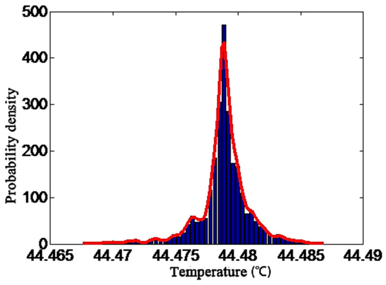
The details of the process are as follows: First, the infrared camera is used to get the surface temperature of the cable joint; then, TPD is obtained according to Equations (1)–(4), as shown in Figure 4. Finally, the defect type and degree of cable are judged based on the characteristic of TPD.

4. Simulation and Results

4.1. Cable Eccentricity

4.1.1. Measurement Precision with Resistor

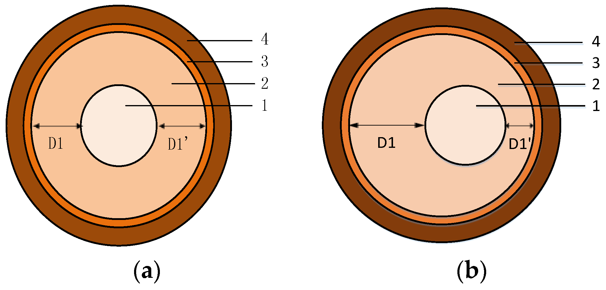
A cross-section of the cable joint is shown in Figure 5, and the degree of insulation eccentricity is defined as $D=\frac{D_1-{D_1}^{\prime }}{2}$, where D₁, D₁′ represents the insulation thickness.

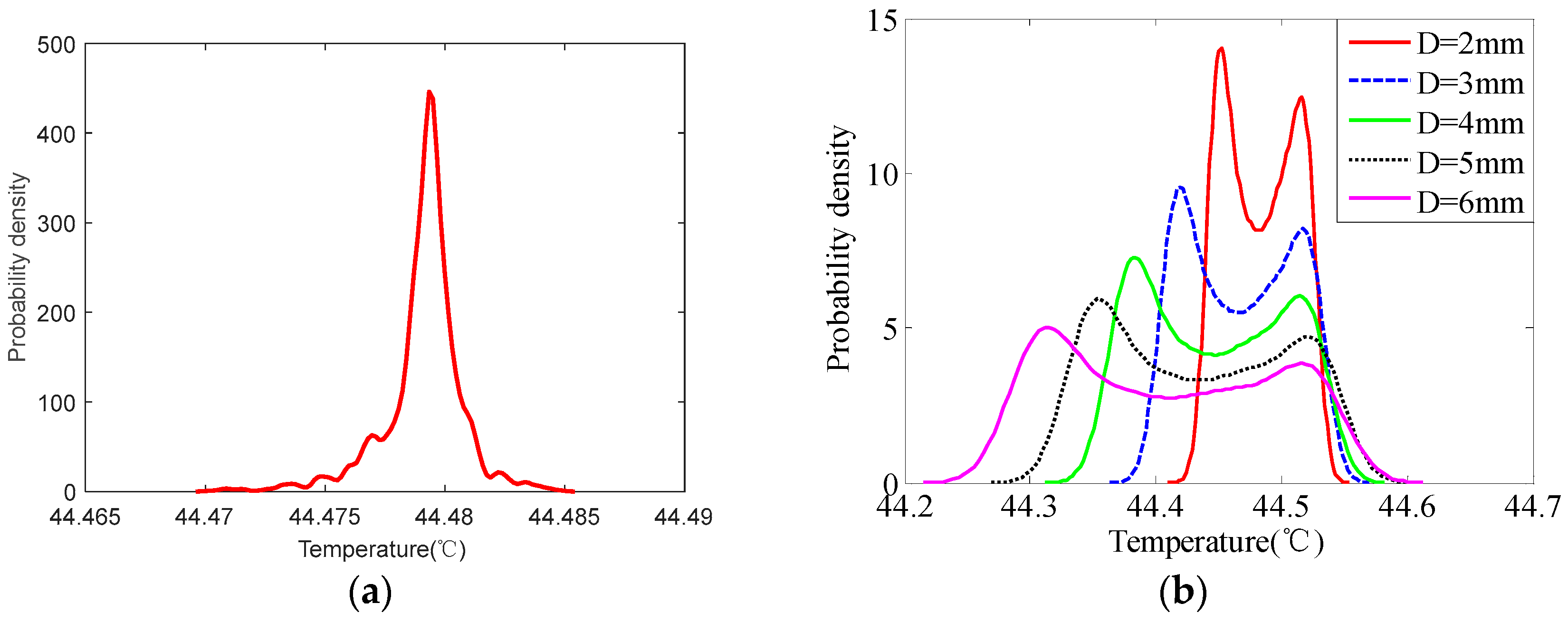
Based on the model of cable joint shown in Figure 1, the temperature distribution was calculated when D = 0 mm, 2 mm, 3 mm, 4 mm, 5 mm, and 6 mm, and the results when D = 3 mm are shown in Figure 6. The temperature distribution is not uniform when the cable joint is eccentric, which is the basis for the detection of cable eccentricity. TPDs under normal and insulation eccentricity are shown in Figure 7.

Comparing Figure 7a,b, it can be seen that under normal conditions, the distribution of cable surface temperature is uniform and the temperature is concentrated at 44.479 °C. When the cable is eccentric, its TPD changes from a single peak to a bimodal wave. In addition, the peak-peak difference increases as the degree of eccentricity increases, and when D changes from 2 mm to 6 mm, the corresponding peak-peak difference increases from 0.06 °C to 0.20 °C.

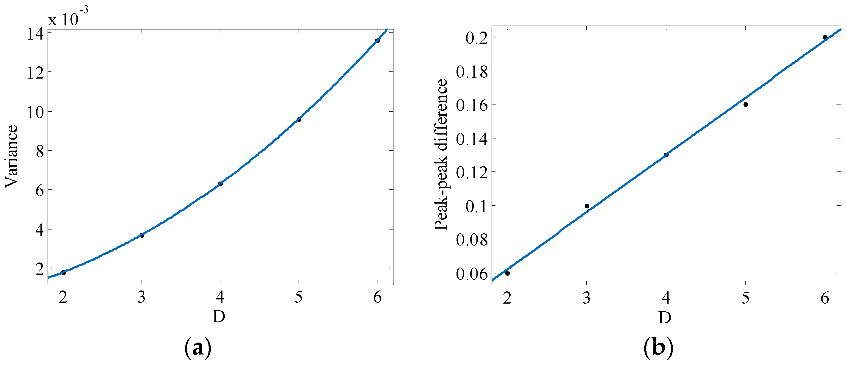
The change rule of the characteristic parameters under different eccentricity is shown in

Table 6. Characteristics of TPD under different eccentricities.

D	Variance	Peak-Peak Difference
0 mm (normal)	2.68 × 10−6	0
2 mm	0.0018	0.06
3 mm	0.0037	0.10
4 mm	0.0063	0.13
5 mm	0.0096	0.16
6 mm	0.0136	0.20

. The variance increases in the form of a quadratic function with increased D. When D increases from 2 to 6 mm, the variance increases from 0.0018 to 0.0136, and the change rule is shown in Figure 8a. The rule can be expressed with the function $s=0.0035D^2-0.00015D+0.0001$, where s is the variance. In addition, the peak-peak difference increases in the form of the first-order function, which is expressed as $P=0.034D-0.006$, where P is the peak-peak difference. When D increases from 2 to 6 mm, the peak-peak difference changes from 0.06 to 0.20, as shown in Figure 8b.

4.1.2. Experimental Verification

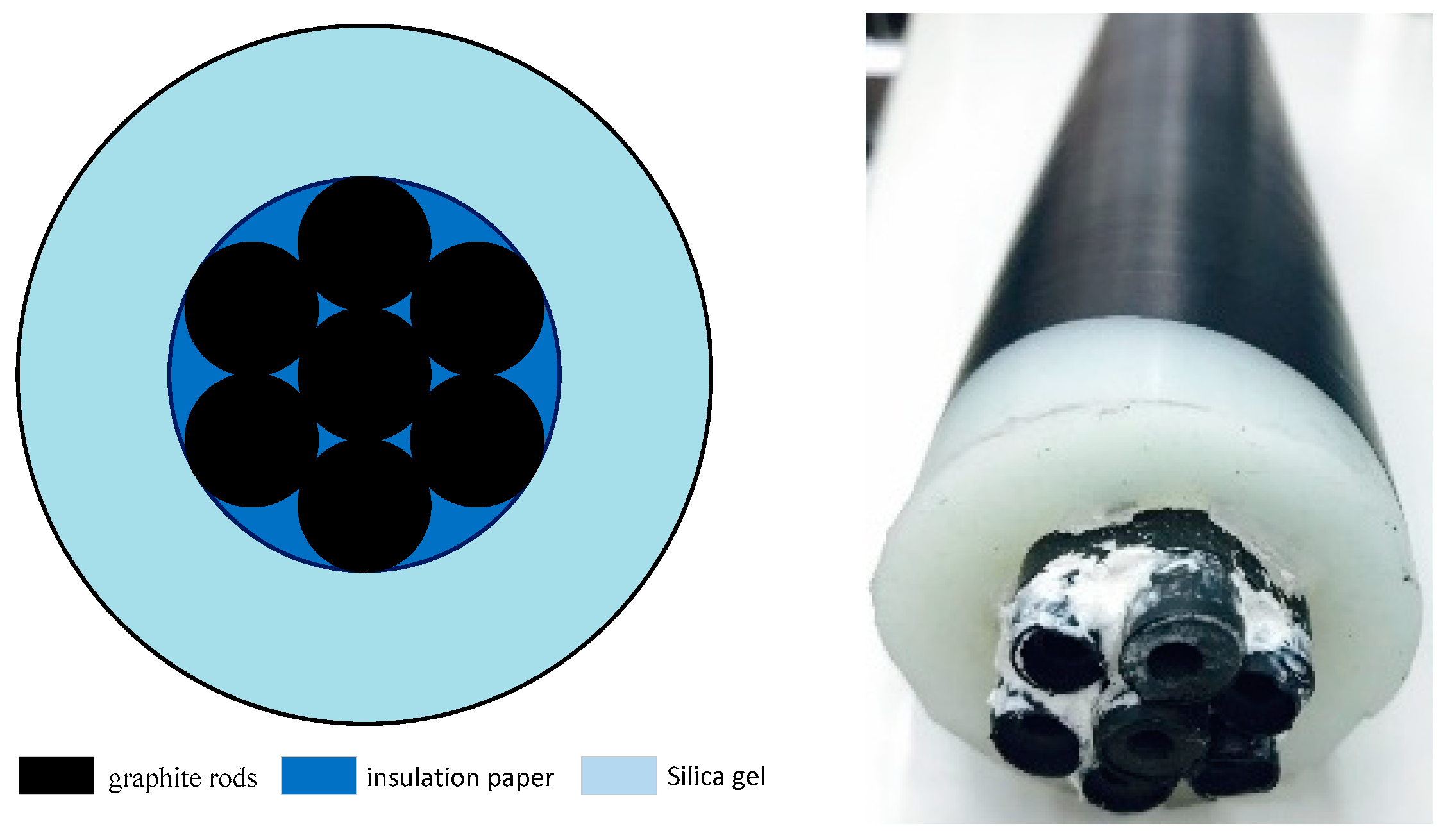
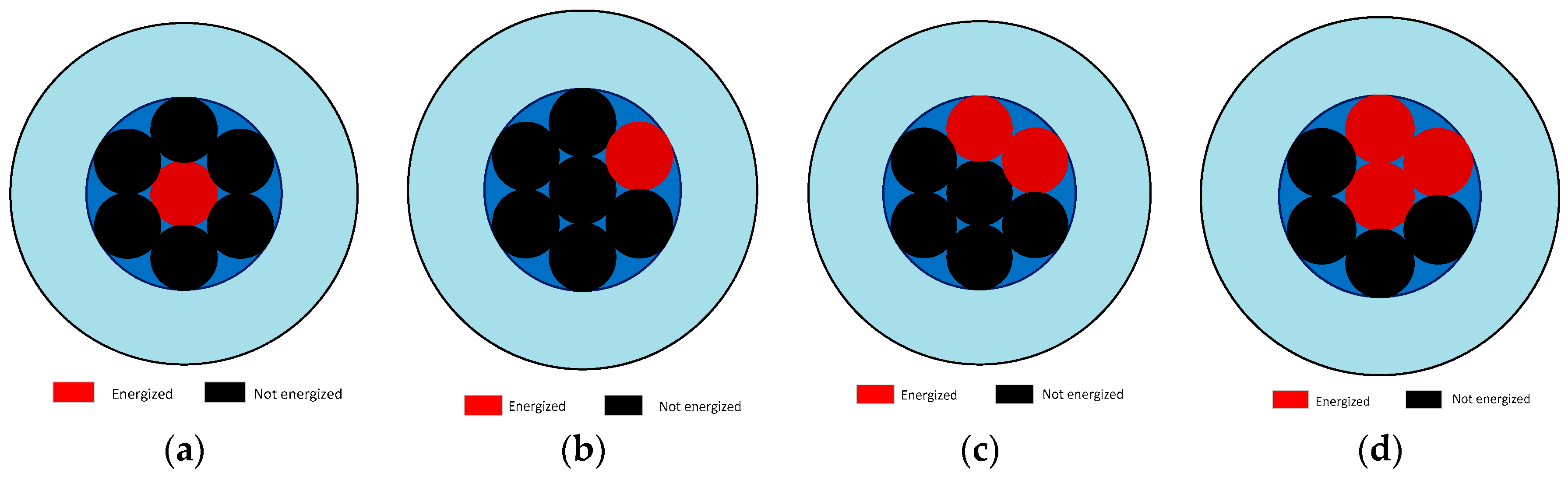
Based on the principle of equal heat source, a surface temperature measurement platform was built. Using graphite rods as a core conductor to simulate the actual operation of large loads not only overcomes the problem of imposing a high load current of 400 A and above in laboratory conditions, but also reduces the cost of the experiment. Figure 9 shows the structure of the analog cable. The resistance of each graphite rod is about 1 Ω.

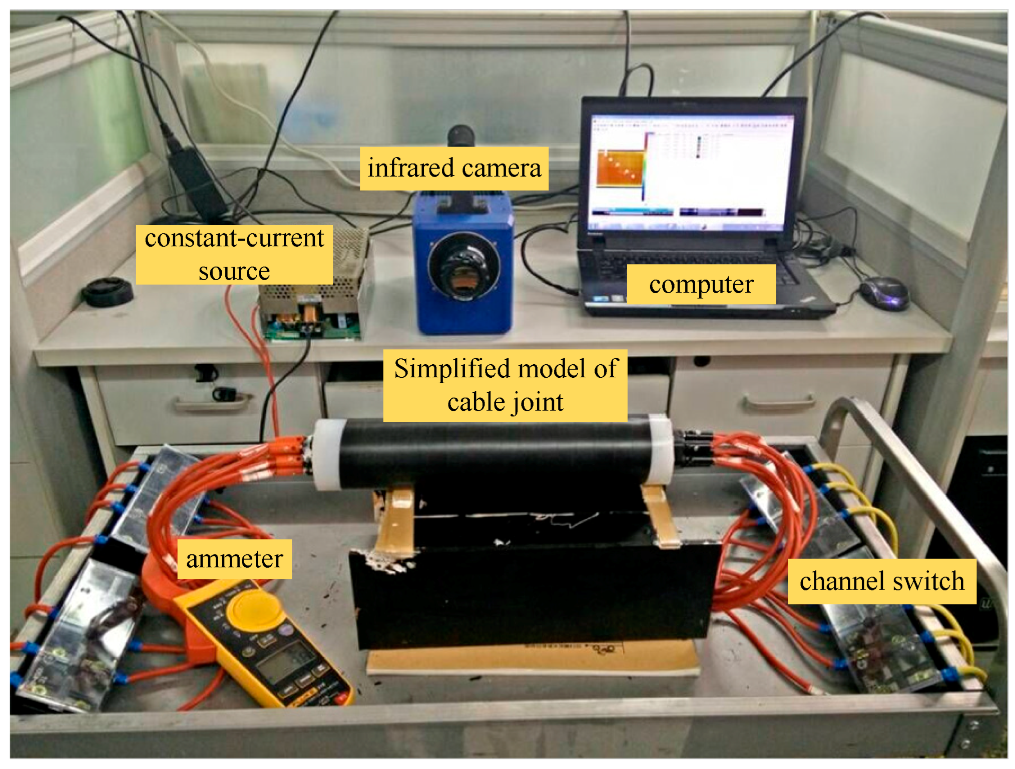
Different degrees of insulation eccentricity were simulated in different parallel ways using the graphite rods, as shown in Figure 10. A 12 V/30 A adjustable constant-current source was used to supply power, and the output current could be adjusted in the range of 5 A to 30 A to ensure the same internal heat. The related data are shown in

Table 7. Internal heat of cable.

Case	Resistance	Current	Energy
Normal	1 Ω	10 A	100 J
Case 1	1 Ω	10 A	100 J
Case 2	0.5 Ω	14 A	98 J
Case 3	0.33 Ω	17 A	95.37 J

. Temperature was measured by an FLIR SC7000 infrared camera, whose accuracy is 0.1 °C. The outer side of the cable and its support parts were painted black so that the radiation coefficient was close to 1. The infrared camera was placed at the same level as the cable and the steady-state temperature data were recorded. The experimental platform is shown in Figure 11.

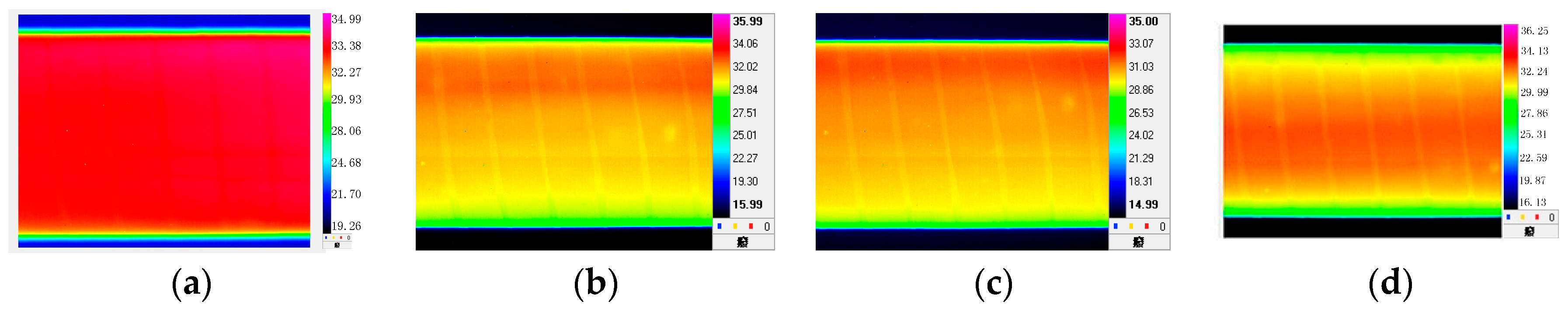
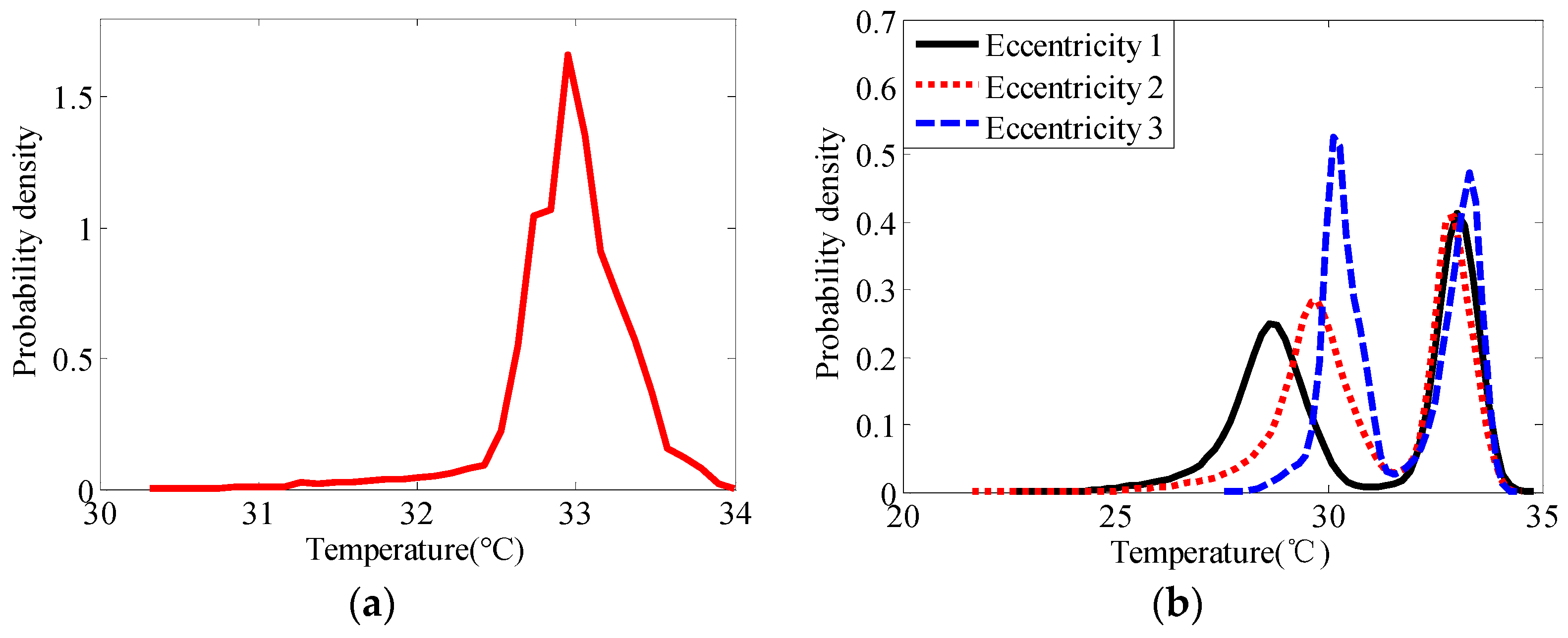
The surface temperature distribution recorded by the infrared thermal imager is shown in Figure 12 and TPDs are shown in Figure 13. Under normal conditions, the surface temperature distribution is uniform and the temperatures are concentrated at 33 °C. When the cable is eccentric, the surface temperature distribution is not uniform. The waveform is distorted from a single peak wave to a bimodal one, and the tendency of the related parameters of waveform is consistent with that obtained in simulation, which proves the feasibility of the proposed method.

4.2. Contact Resistance

This method can not only be applied to cable eccentricity testing but also be used to analyze the degree of excess contact resistance.

Due to crimping process defects, the thermal loss of cable joint increases, resulting in a surface temperature distribution difference. In order to quantitatively characterize the influence of contact resistance, the contact coefficient K is defined as K = R₁/R₂, where R₁ = $\frac{1}{{\sigma }_2}\frac{1}{\pi r_2^2}$ and R₂ = $\frac{1}{{\sigma }_1}\frac{1}{\pi r_1^2}$. R₁ is the resistance of the connection portion and R₂ is the conductor resistance of a cable body of the same length. A schematic diagram of contact coefficient is shown in Figure 14, and the formula is expressed as Equation (7).

$$K=\frac{\frac{1}{{\sigma }_2}\frac{1}{\pi r_2^2}}{\frac{1}{{\sigma }_1}\frac{1}{\pi r_1^2}}=\frac{{\sigma }_1}{{\sigma }_2}{\left(\frac{r_1}{r_2}\right)}^2$$

(7)

Based on the model of cable joint shown in Figure 1, the temperature distribution was calculated when K = 1, 3, 5, 7, 11, and the results when K = 5 are shown in Figure 15. Surface temperatures of the cable joint and the cable body are different, so the contact coefficient can be determined by the temperature difference between them.

The TPDs of the cable with different K values are shown in Figure 16. The peak-peak difference decreases gradually with the increase of K, and changes gradually from a bimodal wave to a unimodal wave (K = 9, K = 11). The variance values and peak-peak differences with different K are shown in

Table 8. Characteristics of TPDs under different K values.

K	Variance	P1	P2	Peak-Peak Difference
K = 1	17.30	38.02	47.49	9.47
K = 3	12.23	40.21	47.88	7.67
K = 5	8.46	42.04	48.44	6.40
K = 7	5.70	44.25	48.89	4.64
K = 9	3.87	46.44	48.90	2.46
K = 11	2.60	48.76	48.76	0

.

Figure 17a shows that the variance decreases in the form of a quadratic function as K increases. When contact coefficient K increases from 1 to 11, variance is reduced from 17.30 to 2.60. The relationship between variance and contact coefficient can be described with $s=0.12K^2-2.88K+19.95$, where s is variance. The peak-peak difference also decreases with the increase of K, and if the contact coefficient K continues to increase, the peak-peak difference will become negative. The function that represents the relationship between the peak-peak difference and the contact coefficient is $P=-0.9258K+10.66$, where P is the peak-peak difference. The change trend is shown in Figure 17b.

To further analyze the reason for the curve distribution in Figure 18, we analyzed the temperature distribution of the cable surface axis with different contact coefficient K, as shown in Figure 18.

Figure 18 shows that when K is small, the temperature at the cable joint is lower than that at the cable body, because the cable joint has a greater heat dissipation area. When K is small, thermal convection plays a major role in the cable joint temperature being significant lower than the body temperature and a low temperature peak, shown in Figure 16. With increased K, the heat yield of cable joint increases gradually, therefore the joint temperature increases gradually and the peak-peak difference reduces gradually. Since contact resistance only changes the heat generation rate and heat conduction in the axial direction becomes weak when the distance from the center of the cable joint is more than 2.5 m, the cable body temperature 2.5 m from the center does not change with K.

5. Conclusions

This paper proposes a method of using infrared temperature measurement and analyzes the regularities of TPD to estimate the type and degree of internal faults of cable, based on a three-dimensional electromagnetic-thermal multiphysics model of power cable. When cable internal faults occur, the distributions of surface temperature probability density curves are different. Combining the characteristic of TPD, a comprehensive judgment can be made to determine the type and degree of cable defects accurately. In addition, an experimental platform was built to verify the method proposed in this paper, and the experimental results are consistent with the simulation results, which verifies the feasibility of the method.

References

- Shaker, Y.O.; EI-Hag, A.H.; Patel, U.; Jayaram, S.H. Thermal modeling of medium voltage cable terminations under square pulses. IEEE Trans. Dielectr. Electr. Insul. 2014, 21, 932–939. [Google Scholar] [CrossRef]
- Xiang, X.; Tu, P.; Zhao, J. Application of fiber Bragg grating sensor in temperature monitoring of power cable joints. In Proceedings of the 2011 International Conference on Electronics, Communications and Control (ICECC), Ningbo, China, 9–11 September 2011; pp. 755–757. [Google Scholar]
- Gan, W.; Wang, Y. Application of the distributed optical fiber grating temperature sensing technology in high-voltage cable. In Proceedings of the 2011 International Conference on Electronic & Mechanical Engineering and Information Technology, Harbin, China, 12–14 August 2011; Volume 9, pp. 4538–4541. [Google Scholar]
- Cui, H.; Xu, Y.; Zeng, J.; Tang, Z. The methods in infrared thermal imaging diagnosis technology of power equipment. In Proceedings of the 2013 IEEE 4th International Conference on Electronics Information and Emergency Communication, Beijing, China, 15–17 November 2013; pp. 246–251. [Google Scholar]
- He, H.; Lee, W.-J.; Luo, D.; Cao, Y. Insulator Infrared Image Denoising Method Based on Wavelet Generic Gaussian Distribution and Map Estimation. In Proceedings of the 2016 IEEE Industry Applications Society Annual Meeting, Portland, OR, USA, 2–6 October 2016. [Google Scholar]
- Chaturvedi, D.K.; Iqbal, M.S.; Pratap, M. Intelligent health monitoring system for three phase induction motor using infrared thermal image. In Proceedings of the 2015 International Conference on Energy Economics and Environment (ICEEE), Noida, India, 27–28 March 2015; pp. 1–6. [Google Scholar]
- Tang, Q.; Liu, J.; Dai, J.; Yu, Z. Theoretical and experimental study on thermal barrier coating (TBC) uneven thickness detection using pulsed infrared thermography technology. Appl. Therm. Eng. 2017, 114, 770–775. [Google Scholar] [CrossRef]
- Tang, Q.; Dai, J.; Bu, C.; Qi, L.; Li, D. Application of infrared thermography for predictive/preventive maintenance of thermal defect in electrical equipment. Appl. Therm. Eng. 2013, 61, 220–227. [Google Scholar]
- Ruan, J.; Liu, C.; Huang, D.; Zhan, Q.; Tang, L. Hot spot temperature inversion for the single-core power cable joint. Appl. Therm. Eng. 2013, 104, 146–152. [Google Scholar] [CrossRef]
- Sturchio, A.; Fioriti, G.; Pompili, M.; Cauzillo, B. Failure rates reduction in SmartGrid MV underground distribution cables: Influence of temperature. In Proceedings of the 2014 AEIT Annual Conference—From Research to Industry: The Need for a More Effective Technology Transfer (AEIT), Trieste, Italy, 18–19 September 2014; pp. 1–6. [Google Scholar]
- Mendes, M.A.; Tonini, L.G.R.; Muniz, P.R.; Donadel, C.B. Thermographic analysis of parallelly cables: A method to avoid misdiagnosis. Appl. Therm. Eng. 2013, 104, 231–236. [Google Scholar] [CrossRef]
- Lei, M.; Liu, G.; Lai, Y.; Li, J.; Li, W.; Liu, Y. Study on thermal model of dynamic temperature calculation of single-core cable based on Laplace calculation method. In Proceedings of the 2010 IEEE International Symposium on Electrical Insulation, San Diego, CA, USA, 6–9 June 2010; pp. 1–7. [Google Scholar]
- Steennis, F.; Wagenaars, P.; van der Wielen, P.; Wouters, P.; Li, Y.; Broersma, T.; Harmsen, D.; Bleeker, P. Guarding MV cables on-line: With travelling wave based temperature monitoring, fault location, PD location and PD related remaining life aspects. IEEE Trans. Dielectr. Electr. Insul. 2016, 23, 1562–1569. [Google Scholar] [CrossRef]
- Fedorov, M.E. Optical Laser Diffraction Transducer for Measuring Single-Wire Electric Cable Eccentricity. IOP Conf. Ser. Mater. Sci. Eng. 2015, 81, 012074. [Google Scholar] [CrossRef]
- Ruzlin, M.M.M.; Shafi, A.H.H.; Basri, A.G.A. Study of cable crimping factors affecting contact resistance of medium voltage cable ferrule and lug. In Proceedings of the 22nd International Conference and Exhibition on Electricity Distribution (CIRED 2013), Stockholm, Sweden, 10–13 June 2013; pp. 1–4. [Google Scholar]
- Luo, H.; Cheng, P.; Liu, H.; Kang, K.; Yang, F.; Yang, Q. Investigation of contact resistance influence on power cable joint temperature based on 3-D coupling model. In Proceedings of the 2016 IEEE 11th Conference on Industrial Electronics and Applications (ICIEA), Hefei, China, 5–7 June 2016; pp. 2265–2268. [Google Scholar]
- Robinson, A.P.; Lewin, P.L.; Sutton, S.J.; Swingler, S.G. Inspection of high voltage cables using X-ray techniques. IEEE Int. Symp. Electr. Insul. 2004, 19, 372–375. [Google Scholar]
- Yang, F.; Cheng, P.; Luo, H.; Yang, Y.; Liu, H.; Kang, K. 3-D thermal analysis and contact resistance evaluation of power cable joint. Appl. Therm. Eng. 2016, 93, 1183–1192. [Google Scholar] [CrossRef]
- Perpiñà, X.; Castellazzi, A.; Piton, M.; Mermet-Guyennet, M.; Millán, J. Failure-relevant abnormal events in power inverters considering measured IGBT module temperature inhomogeneities. Microelectron. Reliab. 2007, 47, 1784–1789. [Google Scholar] [CrossRef]
- Comaniciu, D.; Ramesh, V.; Meer, P. Kernel-Based Object Tracking. IEEE Trans. Pattern Anal. Mach. Intell. 2003, 40, 564–575. [Google Scholar] [CrossRef]
- Pană, C.; Severi, S.; de Abreu, G.T.F. An adaptive approach to non-parametric estimation of dynamic probability density functions. In Proceedings of the 2016 13th Workshop on Positioning, Navigation and Communications (WPNC), Bremen, Germany, 19–20 October 2016; pp. 1–4. [Google Scholar]
Figure 1.
Axial cross-section model of cable joint.
Figure 2.
Infrared images.
Figure 3.
Illustration of gray level distribution corresponding to temperature image.
Figure 4.
Thermal probability density (TPD) under normal conditions.
Figure 5.
Cable cross-section diagram: (a) normal, (b) eccentricity.
Figure 6.
Temperature distribution when D = 3 mm.
Figure 7.
TPDs of cable under (a) normal and (b) insulation eccentricity conditions.
Figure 8.
Relationship between characteristics of TPD and cable eccentricity: (a) variance, (b) peak-peak difference.
Figure 9.
Structure of the cable model.
Figure 10.
Structure of the insulation eccentricity cables: (a) normal, (b) case 1, (c) case 2, (d) case 3.
Figure 11.
Schematic diagram of the experimental scheme.
Figure 12.
Infrared images of cable surface temperature: (a) normal, (b) case 1, (c) case 2, (d) case 3.
Figure 13.
TPDs in experiment under different insulation eccentricities: (a) normal, (b) eccentricity.
Figure 14.
Structure and equivalent model of cable conductor connection.
Figure 15.
Temperature distribution of K = 5.
Figure 16.
TPDs of cable with different K values.
Figure 17.
Relationship between characteristics of TPD and K: (a) variance, (b) peak-peak difference.
Figure 18.
Surface axial temperature distribution curve of cable with different K values.