Designing a Reliable and Congested Multi-Modal Facility Location Problem for Biofuel Supply Chain Network

Abstract

This study presents a mathematical model that designs a reliable multi-modal transportation network for a biofuel supply chain system while site-dependent facility failure and congestion are taken into consideration. The proposed model locates the multi-modal facilities and biorefineries and determines the optimal production, storage, and routing plans in such a way that the overall system cost is minimized. We propose a hybrid Constraint generation-based Rolling horizon algorithm to solve this challenging $\mathcal{NP}$-hard problem. The performance of this algorithm is tested in a example case study with numerical analysis showing that the hybrid algorithm can find near-optimal solutions to large-scale problem instances in a reasonable amount of time. Results indicate that the effect of congestion reduces the usage of multi-modal facilities in the biofuel supply chain network while bio-refineries and multi-modal facilities tend to move away from coastal areas when disruption probabilities are taken into consideration.

1. Introduction

The biofuel industry in the United States is growing at a fast pace. Bioethanol production increased from 1.15 billion gallons in 2000 to 15.08 billion gallons in 2017 [1]. Simultaneously, biodiesel production is increasing sharply, producing almost 107 million gallons only in September, 2015. The new US Renewable Fuels Standard (RFS) sets an annual production target of 36 billion gallons of biofuel, consisting of mainly ethanol and biodiesel, by 2022 [2]. Designing a robust biofuel supply chain network is of special importance, given this projected increase in production. The efficiency and reliability of a biofuel supply chain network will be determined by the performance of an integrated biofuel production and transportation system that not only operates well under normal conditions but also hedges against risk of disruption and/or congestion [3,4].

Designing an efficient and robust biofuel supply chain is challenging due to the physical characteristics of biomass (e.g., seasonality, uncertainty, and widely dispersed supply) [5]. For instance, corn stover is only available from early September to November, while woody biomass is available all year round with the exception of three months in the winter. Overall, early September through late November is the peak biomass production season in the US, and more biomass is expected to ship through multi-modal facilities during those time periods of the year. This peak seasonality not only congests the facilities, but also impacts overall biomass supply chain efficiency [6]. Moreover, there is a significant increase in grain transportation for U.S. railways during the last few years. Grain transportation increased by 26 percent in 2014 compared to 2013 and 25 percent compared to the average of the three years (2011–2013) [7]. This increase in grain transportation has a ripple effect on the overall supply chain structure, resulting in increased road traffic and air pollution. Another detrimental effect of congestion is that the quality of biomass degrades with time and may become unusable if the time needed to reach destination points increases [6]. Therefore, congestion must be taken into consideration when designing a biofuel supply chain.

Congestion management has received attention from the research community over the last few years. Grove and O’Kelly [8] first investigated the relationship between hub-and-spoke networks and congestion by simulating the daily operations of a single assignment hub-and-spoke network. Elhedhli and Hu [9] introduced a non-linear congestion term in the objective function of an uncapacitated hub location problem which they later extended to a capacitated hub-and-spoke network design problem [10]. Most recently, Camargo et al. [11] modeled the congestion as a convex cost function and developed a mixed integer nonlinear programming model for a multiple allocation hub-and-spoke network design problem. The authors successfully solved as many as 81 nodes by using a generalized Benders decomposition algorithm. A handful of studies [12,13] focused on the impact of congestion under demand uncertainty; however, this area remains vastly uninvestigated by the biofuel supply chain research community where feedstock seasonality and uncertainty can cause severe network congestion. Bai et al. [14] first introduced the traffic congestion factor in the traditional facility location model to decide the optimal location of refineries and the flow of biomass and ethanol in the transportation network. Later, Hajibabai and Ouyang [15] proposed an integrated mathematical model that focused on minimizing the total cost of facility construction, roadway capacity expansion, and biomass/biofuel transportation delay due to congestion. Few studies elaborated on the significance of congestion pricing on various aspects of decision making. Interested readers can refer to the studies by De Palma and Lindsay [16] and Friesz et al. [17] for more details.

Similar to facility congestion, transportation infrastructure, particularly those bearing multi-modal traffic, may be vulnerable to various disruption risks, such as natural disasters (e.g., 2005 Hurricane Katrina, 2008 China and 2009 Haiti earthquake [18,19]) and human-caused disasters (e.g., 2003 US Northeast blackout, 2010 Gulf of Mexico oil spill [20,21]). Furthermore, some areas are recognized as disaster prone areas. For instance, Figure 1 shows that in total 39 different storms affected North Carolina between 2000 and 2008 [22].

Daskin [23] was the first to consider facility unavailability in a maximal covering location problem. The author then extended this study to formulate a maximum expected covering location problem where the demand is not readily met as the facilities capable of fulfilling the demand is busy in serving other customers [24]. This work was further extended by Drezner [25] to develop a reliable p-median facility location problem. Snyder and Daskin [26] proposed an integer programming model for the stochastic fixed charge p-median location problem assuming that the facility disruptions occur independently and with equal probability. Later, Cui et al. [27] extended this work by creating both discrete and continuous models where disruption probabilities are dependent on specific sites. Location design models explored by An et al. [28] for several types of emergency service facilities under probabilistic facility disruption risks to reduce the expected cost of losing service. Parvaresh et al. [29] developed a bi-level game model by formulating a multiple allocation p-hub median problem under intentional disruptions. The primary objective of the study was to determine the hubs, failure of which would diminish service efficiency to the greatest extent. Darayi et al. [30] integrated a multi-commodity network flow formulation with an economic interdependency model to quantify the multi-industry impacts of a disruption in a transportation network. The goal of the study was to measure the vulnerability of a multimodal freight transportation network and assess the importance of network components using the vulnerability analysis.

In the biofuel supply chain literature, the number of studies that consider the effect of biorefinery disruption are scarce. Li et al. [31], Wang and Ouyang [32], and Huang and Pang [33] studied failure risks at biorefineries but ignored the fact that disruption can simultaneously occur at multi-modal facilities. Please note that the biofuel supply chain system from biomass production to bio-refineries can be viewed as a hub-and-spoke transportation network. Please note that most of the prior studies (e.g., [34,35,36,37,38,39,40]) assume that the transportation hubs are always functioning and will never fail, which cannot adequately describe the real-world scenarios. A few studies focus on managing and rescheduling rail and port operations during different disrupted scenarios (e.g., [41,42,43]). A system dynamics approach was proposed by Peng et al. [44] to analyze the behavior of disrupted disaster relief supply chain by simulating the uncertainties associated with predicting post-seismic road network and delayed information. Kim and O’Kelly [45] proposed a single and multiple allocation reliable p-hub location model where each arc and each hub is assigned a reliability factor. Marufuzzaman et al. [46] and Marufuzzaman and Eksioglu [47] proposed an optimization model to examine the impact of disruption risks at multi-modal facilities and biorefineries in a biofuel supply chain network. Poudel et al. [48] proposed a pre-disaster planning model while considering the failure probability of links between multi-modal facilities. Bai et al. [49] investigated the impact of failure risks at biorefineries and at intermediate transportation hubs in the biofuel supply chain network. Through experimentation it was observed that the number of biorefineries was directly proportional to the probability of disruption. Authors also found that the cost of a biorefinery had significant impact on the optimal decisions.

To fill this gap in the literature, this paper studies the impact of facility disruption along with network congestion in the context of a biofuel supply chain network. We propose an optimizationmodel that determines the optimal location of biorefineries and multi-modal facilities while simultaneously determining the production, storing, and routing plans in such a way that the overall system cost is minimized under normal and disrupted scenarios. To tackle the complexity of this problem, we develop a hybrid decomposition algorithm that combines Constraint generation algorithm with a Rolling horizon heuristic. The proposed algorithm is validated by developing a example case study. We use the states ofMississippi and Alabama as a testing ground for this study. The outcomes of this study provide several managerial insights such as the optimal deployment of multi-modal facilities and biorefineries, amount of biomass transported via multi-modal facilities/highways, and the impact of disruption and congestion on biofuel supply chain performance.

The paper is organized as follows: Section 2 formulates the mathematical model; Section 3 introduces the solution algorithms; Section 4 presents numerical results and draw managerial insights; and finally, Section 5 provides conclusions and future research directions.

2. Problem Description and Model Formulation

The main objective of this paper is to build a reliable biofuel supply chain network that takes multi-modal facility disruption along with facility congestion into account. The aim is to build biorefineries and use multi-modal facilities among candidate facility locations to produce, store, and transport biomass/biofuel in such a way that the overall system cost is minimized under both normal and disrupted scenarios. Additionally, our model attempts to minimize facility congestion caused by feedstock seasonality and facility unavailability. Figure 2 presents the structure of the supply chain network consisting of two biomass supplier, three multi-modal facilities, two biorefineries, and three markets for biofuel production.

2.1. Nonlinear Problem Formulation

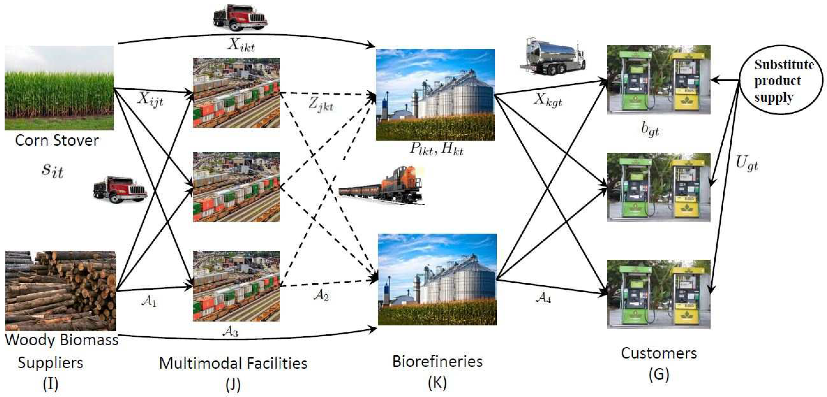
Let us denote a biofuel supply chain network $\mathbb{G}(\mathcal{N},\mathcal{A})$, where $\mathcal{N}$ denotes the set of nodes and $\mathcal{A}$ denotes the set of arcs. Set $\mathcal{N}$ consists of the set of harvesting sites $\mathcal{I}$, the set of candidate multi-modal facilities $\mathcal{J}$, the set of biorefineries $\mathcal{K}$, and the set of markets for biofuel $\mathcal{G}$ i.e., $\mathcal{N}=\mathcal{I}\cup \mathcal{J}\cup \mathcal{K}\cup \mathcal{G}$. Similarly, set $\mathcal{A}$ can be partitioned into four disjoint subsets i.e., $\mathcal{A}={\mathcal{A}}_1\cup {\mathcal{A}}_2\cup {\mathcal{A}}_3\cup {\mathcal{A}}_4$ where, ${\mathcal{A}}_1$ represents the set of arcs connecting harvesting sites $\mathcal{I}$ with multi-modal facilities $\mathcal{J}$, ${\mathcal{A}}_2$ represents the set of arcs connecting multi-modal facilities $\mathcal{J}$ with biorefineries $\mathcal{K}$, ${\mathcal{A}}_3$ represents the set of arcs that directly connect harvesting sites $\mathcal{I}$ with biorefineries $\mathcal{K}$, and ${\mathcal{A}}_4$ represents the set of arcs connecting biorefineries $\mathcal{K}$ with markets $\mathcal{G}$.

Transportation distance along arcs ${\mathcal{A}}_1$ are relatively short; therefore, trucks are preferred to ship biomass along these arcs and its unit transportation cost is denoted by $c_{ijt}$. On the other hand, transportation distance along with shipping volumes in arcs $(j,k)\in {\mathcal{A}}_2$ are high. Thus, transportation mode such as rail can be used to ship biomass along these arcs. Cargo containers are usually used to transport biomass between the multi-modal facilities, and the loading and unloading of biomass in the cargo container incurs a fixed cost of ${\xi }_{jkt}$. The unit cost along arcs $(j,k)\in {\mathcal{A}}_2$ are denoted by $c_{jkt}$. Therefore, the unit transportation cost along arcs $\{(i,j),(j,k)\}$ can be represented by $c_{ijkt}$=$c_{ijt}$+$c_{jkt}$. We further denote $c_{ikt}$ as the unit truck transportation cost of biomass along arcs $(i,k)\in {\mathcal{A}}_3$. These arcs are preferred when the harvesting sites $i\in \mathcal{I}$ are located close to the biorefineries $k\in \mathcal{K}$ and thus, direct shipments of biomass using trucks are considered cheaper over multi-modal facilities. Finally, trucks are used to ship biofuel along arcs ${\mathcal{A}}_4$ by incurring a unit cost of $c_{kgt}$.

Let us consider $l\in \mathcal{L}$ be the set of capacities for multi-modal facilities and biorefineries and $\mathcal{T}$ be the set of time periods. In this model, we denote $s_{it}$ as the amount of biomass available at site $i\in \mathcal{I}$ in time $t\in \mathcal{T}$ and $b_{gt}$ as the demand for biofuel at market $g\in \mathcal{G}$ in time period $t\in \mathcal{T}$. The unmet biofuel demand at market $g\in \mathcal{G}$ in time period $t\in \mathcal{T}$ can be substituted by paying a unit penalty cost of ${\pi }_{gt}$. If the unit cost of delivering biofuel exceeds this threshold cost (${\pi }_{gt}$), it will be beneficial to use substitution rather than producing biofuel at a higher cost. Locating a biorefinery of capacity $l\in \mathcal{L}$ at each location $k\in \mathcal{K}$ incurs a fixed set up cost ${\Psi }_{lk}$. Similarly, using a multi-modal facility of capacity $l\in \mathcal{L}$ at each location $j\in \mathcal{J}$ in time period $t\in \mathcal{T}$ costs ${\eta }_{ljt}$. Some other key parameters used in the model formulation are: $\varphi$ as the conversion rate (ton/gallon) from raw biomass to biofuel; biofuel inventory holding cost $h_{kt}$, and biofuel production cost $p_{lkt}$.

We assume that each facility $j\in \mathcal{J}\bigcup \mathcal{K}$ can disrupt independently in a given time period $t\in \mathcal{T}$. The corresponding site-dependent failure probability is denoted by ${\{q_{jt}\}}_{j\in \mathcal{J}\bigcup \mathcal{K},t\in \mathcal{T}}$. When either multimodel facility or biorefinery disrupts, we assume that the biomass will be routed through an emergency carrier by paying an additional penalty cost which is much higher than the regular transportation cost. To capture this case, we assume that the emergency carrier will cost $\beta (\beta >1)$ times more than the regularly scheduled cost $c_{ijkt}$.

Table 1. Description of the sets.

Symbol	Description
$\mathcal{I}$	Set of harvesting sites (farms)
$\mathcal{J}$	Set of multi-modal facilities
$\mathcal{K}$	Set of potential locations for biofuel plants
$\mathcal{G}$	Set of markets
$\mathcal{L}$	Set of capacities
$\mathcal{T}$	Set of time periods

and

Table 2. Input parameters.

Symbol	Description
${\eta }_{ljt}$	Fixed cost of using a multi-modal of capacity $l\in \mathcal{L}$ at location $j\in \mathcal{J}$ in time period $t\in \mathcal{T}$
${\Psi }_{lk}$	Fixed cost of opening a biorefinery of capacity $l\in \mathcal{L}$ at location $k\in \mathcal{K}$
${\xi }_{jkt}$	Fixed cost of a cargo container for transporting biomass along arc $(j,k)\in {\mathcal{A}}_2$ in period $t\in \mathcal{T}$
$c_{lkt}$	Unit flow cost along arc $(l,k)\in \mathcal{A}$ in period $t\in \mathcal{T}$
$p_{lkt}$	Unit production cost at a biofuel plant of size $l\in \mathcal{L}$ located at $k\in \mathcal{K}$ in period $t\in \mathcal{T}$
$h_{kt}$	Unit inventory cost at biofuel plant $k\in \mathcal{K}$ in period $t\in \mathcal{T}$
${\pi }_{gt}$	Unit penalty cost of not satisfying demand of market $g\in \mathcal{G}$ in period $t\in \mathcal{T}$
$s_{it}$	Amount of biomass available at site $i\in \mathcal{I}$ in period $t\in \mathcal{T}$
$b_{gt}$	biofuel demand of market $g\in \mathcal{G}$ in period $t\in \mathcal{T}$
$c_{lj}^{cap}$	Biomass storage/handling capacity of an multi-modal facility of size $l\in \mathcal{L}$ at location $j\in \mathcal{J}$
$h_{lk}^{cap}$	Biomass storage capacity of a biofuel plant of size $l\in \mathcal{L}$ at location $k\in \mathcal{K}$
$v^{cap}$	Cargo container capacity
$p_{lk}^{cap}$	Production capacity of a biofuel plant of size $l\in \mathcal{L}$ at location $k\in \mathcal{K}$
$\varphi$	Conversion rate from biomass to biofuel
$c_0$	Congestion factor
$q_{jt}$	Failure probability of multi-modal facility $j\in \mathcal{J}\bigcup \mathcal{K}$ in time period $t\in \mathcal{T}$

summarize the notation that we use in this model. We now define the following location and allocation decision variables for our optimization problem.

The first set of decision variables $\mathbb{Y}:={\{Y_{ljt}\}}_{l\in \mathcal{L},j\in \mathcal{J},t\in \mathcal{T}}\cup {\{Y_{lk}\}}_{l\in \mathcal{L},k\in \mathcal{K}}$ determine the size and location to use/open multi-modal facilities and biorefineries, i.e.,

$$Y_{ljt}=\left\{\begin{array}{cc}1\hfill & \mathrm{if} \mathrm{the} \mathrm{multi-modal} \mathrm{facility} j \mathrm{of} \mathrm{capacity} l \mathrm{is} used \mathrm{in} \mathrm{time} \mathrm{period} t\hfill \\ 0\hfill & \mathrm{otherwise};\hfill \end{array}\forall l\in \mathcal{L};j\in \mathcal{J};t\in \mathcal{T}.\right.$$

$$Y_{lk}=\left\{\begin{array}{cc}1\hfill & \mathrm{if} \mathrm{a} \mathrm{biorefinery} \mathrm{of} \mathrm{capacity} l \mathrm{is} \mathrm{opened} \mathrm{at} \mathrm{location} k\hfill \\ 0\hfill & \mathrm{otherwise};\hfill \end{array}\forall l\in \mathcal{L};k\in \mathcal{K}.\right.$$

The second set of variables $\mathbb{Z}:={\{Z_{jkt}\}}_{j\in \mathcal{J},k\in \mathcal{K},t\in \mathcal{T}}$ identifies the number of containers used between multi-modal facilities j and k in period t. The remaining set of decision variables determine how to route, produce, and store the biomass in the biofuel supply chain network. Let $\mathbb{X}:={\{X_{ijkt}\}}_{i\in \mathcal{I},j\in \mathcal{J},k\in \mathcal{K},t\in \mathcal{T}}\cup {\{X_{ikt}\}}_{i\in \mathcal{I},k\in \mathcal{K},t\in \mathcal{T}}\cup {\{X_{kgt}\}}_{k\in \mathcal{K},g\in \mathcal{G},t\in \mathcal{T}}$ denote the flow of biomass through the multi-modal facilities and highways to biorefineries, and biofuel from biorefineries to the customer demand points. Variables $\mathbb{P}:={\{P_{lkt}\}}_{l\in \mathcal{L},k\in \mathcal{K},t\in \mathcal{T}}$ represent the amount of biofuel produced at biorefinery k of size l in period t. Variables $\mathbb{H}:={\{H_{kt}\}}_{k\in \mathcal{K},t\in \mathcal{T}}$ represent the amount of biomass stored at biorefinery k in period t, and $\mathbb{U}:={\{U_{gt}\}}_{g\in \mathcal{G},t\in \mathcal{K}}$ represents the amount of unsatisfied demand in market g in period t. Multi-modal facilities are congested during the peak harvesting seasons of biomass (early September till late November). This congestion in multi-modal facility leads to a dramatic increase in the total supply chain cost. The impact of congestion on total cost becomes more severe when the total flow of feedstock $X_{ijkt}$ approaches the capacity $c_{lj}^{cap}$ of a multi-modal facility $j\in \mathcal{J}$ which is modeled here as $M/M/1$ queuing system. Under steady-state conditions, the system-wide average waiting time for the entire network can be represented as ${\sum }_{j\in \mathcal{J}}{\sum }_{t\in \mathcal{T}}\left(\frac{{\sum }_{i\in \mathcal{I}}{\sum }_{k\in \mathcal{K}}{X}_{ijkt}}{{\sum }_{l\in \mathcal{L}}{c}_{lj}^{cap}{Y}_{ljt}-{\sum }_{i\in \mathcal{I}}{\sum }_{k\in \mathcal{K}}{X}_{ijkt}}\right)$ [10]. Here, for a facility $j\in \mathcal{J}$, when the amount of feedstock $X_{ijkt}$ increases, the ratio of the equation will increase exponentially which will address the impact of congestion realistically in the model formulation. Now, considering $c_0$ as the congestion factor, the system-wide congestion cost becomes ${\sum }_{j\in \mathcal{J}}{\sum }_{t\in \mathcal{T}}{c}_0\left(\frac{{\sum }_{i\in \mathcal{I}}{\sum }_{k\in \mathcal{K}}{X}_{ijkt}}{{\sum }_{l\in \mathcal{L}}{c}_{lj}^{cap}{Y}_{ljt}-{\sum }_{i\in \mathcal{I}}{\sum }_{k\in \mathcal{K}}{X}_{ijkt}}\right)$. This non-linear cost function is now added in the objective function to account for the congestion cost. The following is an Mixed-Integer Nonlinear Programming (MINLP) formulation of the problem referred to as model $[\mathbf{DR}]$.

$$\begin{array}{cc}\hfill [\mathbf{DR}]\underset{\mathbf{Y},\mathbf{Z},\mathbf{P},\mathbf{H},\mathbf{U}}{Minimize}& \sum _{l\in \mathcal{L},k\in \mathcal{K}}{\Psi }_{lk}{Y}_{lk}+\sum _{t\in \mathcal{T}}(\sum _{l\in \mathcal{L},j\in \mathcal{J}}{\eta }_{ljt}{Y}_{ljt}+\sum _{(j,k)\in {\mathcal{A}}_2}{\xi }_{jkt}{Z}_{jkt}+\sum _{l\in \mathcal{L},k\in \mathcal{K}}{p}_{lkt}{P}_{lkt}+\sum _{k\in \mathcal{K}}{h}_{kt}{H}_{kt}+\hfill \\ & \sum _{i\in \mathcal{I},j\in \mathcal{J},k\in \mathcal{K}}{c}_{ijkt}((1-q_{jt})(1-q_{kt})X_{ijkt}+\beta (q_{jt}+q_{kt}-q_{jt}{q}_{kt})X_{ijkt})+\sum _{(i,j)\in {\mathcal{A}}_3\bigcup {\mathcal{A}}_4}{c}_{ijt}{X}_{ijt}\hfill \\ & +\sum _{j\in \mathcal{J}}{c}_0\left(\frac{{\sum }_{i\in \mathcal{I}}{\sum }_{k\in \mathcal{K}}{X}_{ijkt}}{{\sum }_{l\in \mathcal{L}}{c}_{lj}^{cap}{Y}_{ljt}-{\sum }_{i\in \mathcal{I}}{\sum }_{k\in \mathcal{K}}{X}_{ijkt}}\right)+\sum _{g\in \mathcal{G}}{\pi }_{gt}{U}_{gt})\hfill \end{array}$$

Subject to

$$\begin{array}{ccc}\hfill \sum _{k\in \mathcal{K}}{X}_{ikt}+\sum _{j\in \mathcal{J},k\in \mathcal{K}}{X}_{ijkt}& \le & s_{it}\forall i\in \mathcal{I},t\in \mathcal{T}\hfill \end{array}$$

(1)

$$\begin{array}{ccc}\hfill \varphi \left[\sum _{i\in \mathcal{I}}{X}_{ikt}+\sum _{(i,j)\in {\mathcal{A}}^1}{X}_{ijkt}+H_{k,t-1}-H_{kt}\right]& =& \sum _{l\in \mathcal{L}}{P}_{lkt}\forall k\in \mathcal{K},t\in \mathcal{T}\hfill \end{array}$$

(2)

$$\begin{array}{ccc}\hfill \sum _{g\in \mathcal{G}}{X}_{kgt}& \le & \sum _{l\in \mathcal{L}}{P}_{lkt}\forall k\in \mathcal{K},t\in \mathcal{T}\hfill \end{array}$$

(3)

$$\begin{array}{ccc}\hfill \sum _{k\in \mathcal{K}}{X}_{kgt}+U_{gt}& =& b_{gt}\forall g\in \mathcal{G},t\in \mathcal{T}\hfill \end{array}$$

(4)

$$\begin{array}{ccc}\hfill \sum _{i\in \mathcal{I},k\in \mathcal{K}}{X}_{ijkt}& \le & \sum _{l\in \mathcal{L}}{c}_{lj}^{cap}{Y}_{ljt}\forall j\in \mathcal{J},t\in \mathcal{T}\hfill \end{array}$$

(5)

$$\begin{array}{ccc}\hfill \sum _{i\in \mathcal{I}}{X}_{ijkt}& \le & v^{cap}{Z}_{jkt}\forall (j,k)\in {\mathcal{A}}_2,t\in \mathcal{T}\hfill \end{array}$$

(6)

$$\begin{array}{ccc}\hfill P_{lkt}& \le & p_{lk}^{cap}{Y}_{lk}\forall l\in \mathcal{L},k\in \mathcal{K},t\in \mathcal{T}\hfill \end{array}$$

(7)

$$\begin{array}{ccc}\hfill H_{kt}& \le & \sum _{l\in \mathcal{L}}{h}_{lk}^{cap}{Y}_{lk}\forall k\in \mathcal{K},t\in \mathcal{T}\hfill \end{array}$$

(8)

$$\begin{array}{ccc}\hfill \sum _{l\in \mathcal{L}}{Y}_{lk}& \le & 1\forall k\in \mathcal{K}\hfill \end{array}$$

(9)

$$\begin{array}{ccc}\hfill \sum _{l\in \mathcal{L}}{Y}_{ljt}& \le & 1\forall j\in \mathcal{J},t\in \mathcal{T}\hfill \end{array}$$

(10)

$$\begin{array}{ccc}\hfill Y_{lk}& \in & \{0,1\}\forall l\in \mathcal{L},k\in \mathcal{K}\hfill \end{array}$$

(11)

$$\begin{array}{ccc}\hfill Y_{ljt}& \in & \{0,1\}\forall l\in \mathcal{L},j\in \mathcal{J},t\in \mathcal{T}\hfill \end{array}$$

(12)

$$\begin{array}{ccc}\hfill Z_{jkt}& \in & Z^{+}\forall j\in \mathcal{J},k\in \mathcal{K},t\in \mathcal{T}\hfill \end{array}$$

(13)

$$\begin{array}{ccc}\hfill X_{ijkt},X_{ikt},X_{kgt},P_{lkt},H_{kt},U_{gt}& \ge & 0\forall l\in \mathcal{L},i\in \mathcal{I},j\in \mathcal{J},k\in \mathcal{K},g\in \mathcal{G},t\in \mathcal{T}\hfill \end{array}$$

(14)

The objective function of [DR] minimizes the total expected system cost under both normal and disrupted conditions. More specifically, the first, second, and third terms represent respectively the total set-up cost of locating biorefineries, usage cost of multi-modal facilities, and the fixed cost associated with transporting cargo containers between the multi-modal facilities. The fourth and fifth terms represent the production and inventory holding cost at the biorefinieries. The sixth term is the regular transportation cost, which is weighted by $(1-q_{jt})(1-q_{kt})$, the probability that both facilities operate normally along each route $(i,j,k)$. When either or both multi-modal facility $j\in \mathcal{J}$ and biorefinery $k\in \mathcal{K}$ disrupt, which occurs at a probability of $(q_{jt}+q_{kt}-q_{jt}{q}_{kt})$, biomass $X_{ijkt}$ will flow through that route at a higher variable cost $\beta c_{ijkt}$. This is reflected by the seventh term of the objective function. The eighth term is regular transportation cost along the arc ${\mathcal{A}}_3$ and ${\mathcal{A}}_4$. The ninth and tenth terms represent the congestion cost and the penalty cost for the biomass supply shortage.

Constraints (1) indicate that the amount of biomass shipped from supplier $i\in \mathcal{I}$ in period $t\in \mathcal{T}$ is limited by its availability. Constraints (2) are the flow conservation constraints at biorefineries. Constraints (3) indicate that the amount of biofuel delivered to the market is limited by the amount produced in period $t\in \mathcal{T}$. Constraints (4) indicate that the demand for biofuel can be fulfilled either through the distribution network or through substitute products available in the market. Constraints (5) indicate that the total amount of biomass shipped through a multi-modal facility is limited by its capacity $c_{lj}^{cap}$. Constraints (6) count the number of containers needed for shipping biomass on each arc $(j,k)\in {\mathcal{A}}_2$. Constraints (7) set biofuel production capacity $(p_{lk}^{cap})$ limitations at a biorefinery. Constraints (8) set biomass storage limitations $(h_{lk}^{cap})$ at a biorefinery. Constraints (9) and (10) ensure that, at most one multi-modal facility/biorefinery of capacity $l\in \mathcal{L}$ is operating in a given location $j\in \mathcal{J}\bigcup \mathcal{K}$. Finally, constraints (11) and (12) are the binary constraints, (13) are the integer constraints, and (14) are the standard non-negativity constraints.

2.2. Model Linearization

The objective function of model [DR] contains a nonlinear congestion cost function. We use the technique proposed by Elhedhli and Wu [10] to linearize this congestion term. To do this, let us now consider a new decision variable $\mathbf{M}:={\{M_{jt}\}}_{j\in \mathcal{J},t\in \mathcal{T}}$ as follows.

$$\begin{array}{c}\hfill M_{jt}=\frac{{\sum }_{i\in \mathcal{I}}{\sum }_{k\in \mathcal{K}}{X}_{ijkt}}{{\sum }_{l\in \mathcal{L}}{c}_{lj}^{cap}{Y}_{ljt}-{\sum }_{i\in \mathcal{I}}{\sum }_{k\in \mathcal{K}}{X}_{ijkt}}\end{array}$$

(15)

Equation (15) can be further reduced as follows:

$$\begin{array}{c}\hfill \sum _{i\in \mathcal{I}}\sum _{k\in \mathcal{K}}{X}_{ijkt}=\left(\frac{M_{jt}}{1+M_{jt}}\right)\sum _{l\in \mathcal{L}}{c}_{lj}^{cap}{Y}_{ljt}=\sum _{l\in \mathcal{L}}{c}_{lj}^{cap}\left(\frac{M_{jt}}{1+M_{jt}}\right)Y_{ljt}\forall j\in \mathcal{J},t\in \mathcal{T}\end{array}$$

We now introduce another continuous variable $\mathbf{R}:={\{R_{ljt}\}}_{l\in \mathcal{L},j\in \mathcal{J},t\in \mathcal{T}}$ as follows:

$$\begin{array}{c}\hfill R_{ljt}=\left(\frac{M_{jt}}{1+M_{jt}}\right)Y_{ljt}\forall l\in \mathcal{L},j\in \mathcal{J},t\in \mathcal{T}\end{array}$$

(16)

Given that ${\sum }_{l\in \mathcal{L}}{Y}_{ljt}=1$, the above equation becomes

$$\begin{array}{c}\hfill \sum _{l\in \mathcal{L}}{R}_{ljt}=\frac{M_{jt}}{1+M_{jt}}\forall j\in \mathcal{J},t\in \mathcal{T}\end{array}$$

(17)

In the condition when $Y_{ljt}=0$ constraints (17) forces $R_{ljt}=0$, which is enforced by using an additional constraints $0\le R_{ljt}\le Y_{ljt}\forall l\in \mathcal{L},j\in \mathcal{J},t\in \mathcal{T}$.

Lemma 1.

The function ${\sum }_{l\in \mathcal{L}}{R}_{ljt}(M_{jt})=\frac{M_{jt}}{1+M_{jt}}$ is concave in $M_{jt}\in (0,\infty )$.

Proof. 

While differentiating the function $R_{ljt}$ w.r.t. $M_{jt}$, we get the first derivative, $\frac{\delta }{\delta M_{jt}}(R_{ljt})=1/{(1+M_{jt})}^2>0$, and the second derivative, $\frac{{\delta }^2}{\delta M_{jt}^2}(R_{ljt})=-2/{(1+M_{jt})}^3<0$. The first derivative is positive while the second derivative is negative and it proves that the function $R_{ljt}(M_{jt})$ is concave in $M_{jt}$. ☐

Lemma 1 shows that function $R_{ljt}(M_{jt})$ is concave and can be approximated by a set of tangent cutting planes as shown below [50]

$$\begin{array}{c}\hfill \frac{M_{jt}}{1+M_{jt}}=Mi{n}_{h\in \mathcal{H}}\left[\frac{M_{jt}}{{\left(1+M_{jt}^h\right)}^2}+{\left(\frac{M_{jt}^h}{1+M_{jt}^h}\right)}^2\right]\end{array}$$

which is equivalent to

$$\begin{array}{c}\hfill \frac{M_{jt}}{1+M_{jt}}\le \frac{M_{jt}}{{\left(1+M_{jt}^h\right)}^2}+{\left(\frac{M_{jt}^h}{1+M_{jt}^h}\right)}^2\forall j\in \mathcal{J},t\in \mathcal{T},h\in \mathcal{H}\end{array}$$

(18)

where ${\{M_{jt}^h\}}_{j\in \mathcal{J},t\in \mathcal{T},h\in \mathcal{H}}$ are the set of points used to approximate Equation (18). The value of ${\{Y_{ljt}\}}_{l\in \mathcal{L},j\in \mathcal{J},t\in \mathcal{T}}$ is finite; therefore, the value that variable ${\{M_{jt}\}}_{j\in \mathcal{J},t\in \mathcal{T}}$ provides is also finite. This implies that the set $\mathcal{H}$ should be finite. Equation (19) is now derived from (17) and (18) as follows:

$$\begin{array}{c}\hfill \sum _{l\in \mathcal{L}}{R}_{ljt}\le \frac{M_{jt}}{{\left(1+M_{jt}^h\right)}^2}+{\left(\frac{M_{jt}^h}{1+M_{jt}^h}\right)}^2\forall j\in \mathcal{J},t\in \mathcal{T},h\in \mathcal{H}\end{array}$$

(19)

The linearized objective function [LDR] for model [DR] now becomes:

$$\begin{array}{cc}\hfill [\mathbf{LDR}]\underset{\mathbf{Y},\mathbf{Z},\mathbf{P},\mathbf{H},\mathbf{U}}{Minimize}& \sum _{l\in \mathcal{L},k\in \mathcal{K}}{\Psi }_{lk}{Y}_{lk}+\sum _{t\in \mathcal{T}}(\sum _{l\in \mathcal{L},j\in \mathcal{J}}{\eta }_{ljt}{Y}_{ljt}+\sum _{(j,k)\in {\mathcal{A}}^2}{\xi }_{jkt}{Z}_{jkt}+\sum _{l\in \mathcal{L},k\in \mathcal{K}}{p}_{lkt}{P}_{lkt}+\sum _{k\in \mathcal{K}}{h}_{kt}{H}_{kt}+\hfill \\ & \sum _{i\in \mathcal{I},j\in \mathcal{J},k\in \mathcal{K}}{c}_{ijkt}((1-q_{jt})(1-q_{kt})X_{ijkt}+\beta (q_{jt}+q_{kt}-q_{jt}{q}_{kt})X_{ijkt})+\sum _{(i,j)\in {\mathcal{A}}_3\bigcup {\mathcal{A}}_4}{c}_{ijt}{X}_{ijt}\hfill \\ & +\sum _{j\in \mathcal{J}}{c}_0{M}_{jt}+\sum _{g\in \mathcal{G}}{\pi }_{gt}{U}_{gt})\hfill \end{array}$$

Subject to (1)–(4), (6)–(13), (19), and

$$\begin{array}{ccc}\hfill \sum _{i\in \mathcal{I},k\in \mathcal{K}}{X}_{ijkt}& \le & \sum _{l\in \mathcal{L}}{c}_{lj}^{cap}{R}_{ljt}\forall j\in \mathcal{J},t\in \mathcal{T}\hfill \end{array}$$

(20)

$$\begin{array}{ccc}\hfill R_{ljt}& \le & Y_{ljt}\forall l\in \mathcal{L},j\in \mathcal{J},t\in \mathcal{T}\hfill \end{array}$$

(21)

$$\begin{array}{ccc}\hfill X_{ijkt},X_{ikt},X_{kgt},P_{lkt},H_{kt},R_{ljt},M_{jt},U_{gt}& \ge & 0\forall l\in \mathcal{L},i\in \mathcal{I},j\in \mathcal{J},k\in \mathcal{K},g\in \mathcal{G},t\in \mathcal{T}\hfill \end{array}$$

(22)

3. Solution Methodology

This section discusses solution techniques for solving the linearized model [LDR]. Our resulting model [LDR] is an extension of the fixed charge, uncapacitated facility location problem which is known to be an $\mathcal{NP}$-hard problem [51]. Therefore, commercial solvers, such as CPLEX, fail to solve the large scale instances of this problem. In this section, we propose solution techniques such as Constraint generation algorithm, Rolling horizon algorithm, and an integration of Constraint generation with Rolling horizon to solve model [LDR]. The aim is to produce a high-quality solution in solving model [LDR] in a reasonable amount of time.

3.1. Constraint Generation Algorithm

In model [LDR], (19) generate large number of constraints. Therefore, it is really challenging to solve model [LDR] while considering all constraints at once. This motivates us to develop a Constraint Generation (CG) algorithm that can efficiently solve model [LDR] despite generating a large number of constraints through (19). The algorithm, extensively studied in [52], proceeds by sequentially solving a series of integer programs with a subset of the constraints obtained from (19) and added thereafter as needed.

The process stops when the algorithm finds a solution for the sub-problem which does not violate any constraints within some accepted tolerance in the full problem [DR]. Otherwise, a new set of points and thus a new set of constraints/cuts are generated which are added to [LDR] in the next iteration.

Let $L{B}^q$ and $U{B}^q$ denote a lower and upper bound of the original problem at iteration q. We further let v[LDR] be the solution of the objective function value of [LDR] and $(Y^q,Z^q,P^q,H^q,U^q)$ be its optimal solution. The following proposition provides the lower bound of the CG algorithm.

Proposition 1.

For any given subset of points ${\{M_{jt}^h\}}_{H^q\subset H}$ (23) provides a lower bound of the optimal objective function value of [DR].

$$\begin{array}{cc}\hfill L{B}^q=& v[\mathbf{LDR}](H^q)\hfill \\ & =\sum _{l\in \mathcal{L},k\in \mathcal{K}}{\Psi }_{lk}{Y}_{lk}^q+\sum _{t\in \mathcal{T}}(\sum _{l\in \mathcal{L},j\in \mathcal{J}}{\eta }_{ljt}{Y}_{ljt}^q+\sum _{(j,k)\in {\mathcal{A}}_2}{\xi }_{jkt}{Z}_{jkt}^q+\sum _{l\in \mathcal{L},k\in \mathcal{K}}{p}_{lkt}{P}_{lkt}^q+\sum _{k\in \mathcal{K}}{h}_{kt}{H}_{kt}^q+\hfill \\ & \sum _{i\in \mathcal{I},j\in \mathcal{J},k\in \mathcal{K}}{c}_{ijkt}((1-q_{jt})(1-q_{kt})X_{ijkt}^q+\beta (q_{jt}+q_{kt}-q_{jt}{q}_{kt})X_{ijkt}^q)+\sum _{(i,j)\in {\mathcal{A}}_3\bigcup {\mathcal{A}}_4}{c}_{ijt}{X}_{ijt}^q\hfill \\ & +\sum _{j\in \mathcal{J}}{c}_0{M}_{jt}^q+\sum _{g\in \mathcal{G}}{\pi }_{gt}{U}_{gt}^q)\hfill \end{array}$$

(23)

Proof. 

[LDR($H^q$)] is the relaxed version of problem [DR]. Thus, the optimal objective function value v[LDR($H^q$)] obtained from Equation (23) provides the lower bound to the optimal objective value of [LDR]. Since problem [LDR] is an approximation for problem [DR], solution v[LDR($H^q$)] will also provide a valid lower bound for optimal objective function value of [DR]. ☐

Proposition 2.

For any given subset of points ${\{M_{jt}^h\}}_{H^q\subset H}$ (24) provides an upper bound for the optimal objective function value of [DR].

$$\begin{array}{cc}\hfill U{B}^q=& \sum _{l\in \mathcal{L},k\in \mathcal{K}}{\Psi }_{lk}{Y}_{lk}^q+\sum _{t\in \mathcal{T}}(\sum _{l\in \mathcal{L},j\in \mathcal{J}}{\eta }_{ljt}{Y}_{ljt}^q+\sum _{(j,k)\in {\mathcal{A}}_2}{\xi }_{jkt}{Z}_{jkt}^q+\sum _{l\in \mathcal{L},k\in \mathcal{K}}{p}_{lkt}{P}_{lkt}^q+\sum _{k\in \mathcal{K}}{h}_{kt}{H}_{kt}^q+\hfill \\ & \sum _{i\in \mathcal{I},j\in \mathcal{J},k\in \mathcal{K}}{c}_{ijkt}((1-q_{jt})(1-q_{kt})X_{ijkt}^q+\beta (q_{jt}+q_{kt}-q_{jt}{q}_{kt})X_{ijkt}^q)+\sum _{(i,j)\in {\mathcal{A}}_3\bigcup {\mathcal{A}}_4}{c}_{ijt}{X}_{ijt}^q\hfill \\ & +\sum _{j\in \mathcal{J}}{c}_0\left(\frac{{\sum }_{i\in \mathcal{I}}{\sum }_{k\in \mathcal{K}}{X}_{ijkt}^q}{{\sum }_{l\in \mathcal{L}}{c}_{lj}^{cap}{Y}_{ljt}^q-{\sum }_{i\in \mathcal{I}}{\sum }_{k\in \mathcal{K}}{X}_{ijkt}^q}\right)+\sum _{g\in \mathcal{G}}{\pi }_{gt}{U}_{gt}^q)\hfill \end{array}$$

(24)

Proof. 

Any solution feasible to [LDR($H^q$)] also provides a feasible solution to [DR] since all the constraints of [DR] are also contained by [LDR($H^q$)]. Thus, the objective function value of [DR] evaluated at $(Y^q,Z^q,P^q,H^q,U^q)$ as shown in Equation (24), provides an upper bound for the optimal objective value of [DR]. ☐

The algorithm continues until the gap between the lower and upper bound falls below a tolerance level $ϵ$; otherwise, a new set of points $\{M_{jt}^{h_{new}}\}$ are generated using the current solution (shown below) and the process continues. The overall algorithm is shown in Algorithm 1.

$$\begin{array}{c}\hfill M_{jt}^{h_{new}}=\frac{{\sum }_{i\in \mathcal{I}}{\sum }_{k\in \mathcal{K}}{X}_{ijkt}^q}{{\sum }_{l\in \mathcal{L}}{c}_{lj}^{cap}{Y}_{ljt}-{\sum }_{i\in \mathcal{I}}{\sum }_{k\in \mathcal{K}}{X}_{ijkt}^q}\end{array}$$

(25)

Algorithm 1 Constraint Generation Algorithm.

$q\leftarrow 1;U{B}^{q-1}\leftarrow +\infty ;L{B}^{q-1}\leftarrow -\infty$

Choose an initial set of points ${\{M_{jt}^h\}}_{h\in H^q}$ to approximate function $\left(\frac{M_{jt}^h}{1+M_{jt}^h}\right)$

while $(U{B}^{q-1}-L{B}^{q-1})/U{B}^{q-1}>\xi$ do

Solve [LDR($H^q$)] and obtain its optimal solution $(Y^q,Z^q,X^q,P^q,H^q,M^q,U^q)$

Update the lower bound: ${LB}^q\leftarrow$ [LDR($H^q$)]

Update the upper bound $UB\leftarrow min\{U{B}^{q-1},UB(Y^q,Z^q,X^q,P^q,H^q,M^q,U^q)\}$ using Equation (24)

Generate a new set of points $M_{jt}^{h_{new}}=\frac{{\sum }_{i\in \mathcal{I}}{\sum }_{k\in \mathcal{K}}{X}_{ijkt}^q}{{\sum }_{l\in \mathcal{L}}{C}_{lj}^{cap}{Y}_{ljt}-{\sum }_{i\in \mathcal{I}}{\sum }_{k\in \mathcal{K}}{X}_{ijkt}^q};\forall j\in \mathcal{J},t\in \mathcal{T}$

$H^{q+1}\leftarrow H^q$ ⋃ $\{M_{jt}^{h_{new}}\}$

$q\leftarrow q+1$

end while

3.2. Rolling Horizon Heuristics

Solving [LDR($H^q$)] is still considered challenging since the problem is a special case of a capacitated facility location problem which is known to be an $\mathcal{NP}$-hard problem [51]. Therefore, in this section we introduce a heuristic approach based on the rolling horizon scheme suggested by Balasubramanian and Grossmann(2004) [53] and Kostina et al. (2011) [54]. This approach decomposes problem [LDR($H^q$)] into a series of smaller subproblems with a few consecutive time periods and solves each subproblem with initial set of points ${\{M_{jt}^h\}}_{j\in \mathcal{J},t\in \mathcal{T},h\in \mathcal{H}}$. The algorithm terminates once all the subproblems are investigated. The overall algorithm is shown in Algorithm 2.

Algorithm 2 Rolling Horizon (RH) Heuristic.

$t_0^r=0$, $r\leftarrow 1$, $N^r$, terminate ← false

while (terminate = false) do

Set:

$Y_{ljt}\in \{0,1\}$ and $Z_{jkt}\in {\mathbb{Z}}^{+}$ for $t_s^0\le t\le t_s^0+N^s$

$0\le Y_{ljt}\le 1$ and $Z_{jkt}\in {\mathbb{R}}^{+}$ for $t>t_s^0+N^s$

Solve the approximate sub-problem [LDR($H^q$)(s)] using CPLEX

if ($t_0>|\mathcal{T}|$) then

stop ← true

else

Fixing the values of ${\{Y_{ljt}\}}_{l\in \mathcal{L},j\in \mathcal{J},t\in \mathcal{T}}$ and ${\{Z_{jkt}\}}_{j\in \mathcal{J},k\in \mathcal{K},t\in \mathcal{T}}$ for $t<t_s^0$

end if

$r\leftarrow r+1$

end while

Let $t_s^0$ denote the starting time for subproblem s and $N^s$ be the total number of time periods on subproblem s. We can set a fixed or variable size of $N^s$ for each subproblem. Each approximate subproblem of the Rolling horizon algorithm is denoted by [LDR$(H^q)(s)$]. Now, for each iteration approximate subproblems are solved by setting variables as:

• $Y_{ljt}\in \{0,1\}$ and $Z_{jkt}\in Z^{+}$ for $t_s^0\le t\le t_s^0+N^s$
• $0\le Y_{ljt}\le 1$ and $Z_{jkt}\in R^{+}$ for $t>t_s^0+N^s$

The values of $Y_{ljt}$ and $Z_{jkt}$ for $t<t_s^0$ are fixed to the values found when solving approximate subproblem $s+1$, and the steps involved on the iteration are as follows.

Step 1:

Initialize starting time period to $t_s^0$, length of time interval to N; set $s\to 1$.

Step 2:

Solve the approximate subproblem [LDR($(H^q)(s)$] using CPLEX.

Step 3:

if $t_0>\left|T\right|$, then Stop; else, set $s\to s+1$, go to Step 2:.

3.3. Constraint Generation with Rolling Horizon Heuristic

We now propose a hybrid algorithm which integrates the Rolling horizon approach within the Constraint generation framework. Solving the subproblems [LDR($H^q$)] of the Constraint generation algorithm is still considered challenging. The motivates us to employ Rolling horizon algorithm to solve the subproblems [LDR($H^q$)] of the Constraint generation algorithm. The aim is to provide high quality feasible solution for subproblem [LDR($H^q$)] in a reasonable amount of time. The steps involved in solving model [DR] using the proposed Constraint Generation with Rolling Horizon Heuristic is shown in Algorithm 3.

Algorithm 3 Constraint Generation with Rolling Horizon Heuristic.

$q\leftarrow 1;U{B}^{q-1}\leftarrow +\infty ;L{B}^{q-1}\leftarrow -\infty$, $t_0^r=0$, $r\leftarrow 1$, $N^r$, terminate ← false

Choose an initial set of points ${\{M_{jt}^h\}}_{h\in H^q}$ to approximate function $\left(\frac{M_{jt}^h}{1+M_{jt}^h}\right)$

while $(U{B}^{q-1}-L{B}^{q-1})/U{B}^{q-1}>\xi$do

while (terminate = false) do

Set:

$Y_{ljt}\in \{0,1\}$ and $Z_{jkt}\in {\mathbb{Z}}^{+}$ for $t_s^0\le t\le t_s^0+N^s$

$0\le Y_{ljtn}\le 1$ and $Z_{jktn}\in {\mathbb{R}}^{+}$ for $t>t_s^0+N^s$

Solve the approximate sub-problem [LDR($H^q$)$(s)$] using CPLEX

if ($t_0>|\mathcal{T}|$) then

stop ← true

else

Fixing the values of ${\{Y_{ljt}\}}_{l\in \mathcal{L},j\in \mathcal{J},t\in \mathcal{T}}$ and ${\{Z_{jkt}\}}_{j\in \mathcal{J},k\in \mathcal{K},t\in \mathcal{T}}$ for $t<t_s^0$

end if

$r\leftarrow r+1$

end while

Obtain optimal solution of $[\mathbf{LDR}(\mathbf{q})] (Y^q,Z^q,X^q,P^q,H^q,M^q,U^q)$

Update the lower bound: ${LB}^q\leftarrow$ [LDR($H^q$)]

Update the upper bound $UB\leftarrow min\{U{B}^{q-1},UB(Y^q,Z^q,X^q,P^q,H^q,M^q,U^q)\}$ using Equation (24)

Generate a new set of points $M_{jt}^{h_{new}}=\frac{{\sum }_{i\in \mathcal{I}}{\sum }_{k\in \mathcal{K}}{X}_{ijkt}^q}{{\sum }_{l\in \mathcal{L}}{C}_{lj}^{cap}{Y}_{ljt}-{\sum }_{i\in \mathcal{I}}{\sum }_{k\in \mathcal{K}}{X}_{ijkt}^q};\forall j\in \mathcal{J},t\in \mathcal{T}$

$H^{q+1}\leftarrow H^q$ ⋃ $\{M_{jt}^{h_{new}}\}$

$q\leftarrow q+1$

end while

4. Case Study

This section presents a computational study on model [DR] to test our algorithms and to draw managerial insights. We use the state of Mississippi and Alabama as a testing ground for our study. The case study demonstrates how the model and the solution algorithms proposed in this study can be applied to a real-world supply chain network design problem.

4.1. Data Description

Biomass Supply and Demand: Biomass availability (i.e., corn stover and woody biomass) in Mississippi and Alabama are obtained from the Knowledge Discovery Framework (KDF) database of United States Department of Energy [55]. Every year these two states produce about 6.85 million tons (MT) of biomass from 99 different counties. The counties that produce more than 10,000 tons of biomass each year are only considered in this study. Figure 3a shows the distribution of the densified biomass available in this region.

We set the total biofuel demand as 500 million gallons per year (MGY) for the planning horizon [7]. We have identified 149 counties from the region as the demand area and the centroid of those counties is considered as the demand point.

Investment Costs: In this study we consider a total of 53 potential multi-modal facilities and 43 potential biorefinery locations. We used existing multi-modal and inter-modal facilities as potential multi-modal facilities. The potential biorefinery locations are selected based on the prior literatures applied to our test region ([37,38]). Figure 3b shows the locations and distribution of potential multi-modal facilities and biorefineries in this region. The annualized fixed cost for a rail ramp of capacity 1.05 million ton per year (MTY) is estimated to be $54,949 per year [56]. Based on this information, we estimate the investment costs for other rail ramp capacities. We consider five different rail ramp capacities (l = 0.55 MTY, 0.65 MTY, 0.75 MTY, 0.85 MTY, and 1.00 MTY). The annualized fixed cost for facilities are considered based on a lifetime span of 30 years and assuming a discount factor of 10%. The annualized fixed costs for a biorefinery with a 45 million gallon per year (MGY) capacity is set to be $1.59 million [46,57]. This cost is estimated based on a lifetime of 20 years, and a discount factor of 15% is assumed. We consider five different biorefinery sizes (l = 20 MGY, 40 MGY, 60 MGY, 100 MGY, and 150 MGY). Please note that the actual fixed cost may vary by location; however, we use a common fixed cost as a reasonable approximation.

Transportation Costs: We consider that truck and rail are the two modes of transportation available for transporting biomass from multiple sources to destination points. Trucks are used to transport biomass from a feedstock supplier $i\in \mathcal{I}$ to a multi-modal facility $j\in \mathcal{J}$. Trucks can further be used to transport biomass directly from a feedstock supplier $i\in \mathcal{I}$ to a biorefiney $k\in \mathcal{K}$ and biofuel from biorefinery $k\in \mathcal{K}$ to market $g\in \mathcal{G}$.

Table 3. Description of the sets and parameters.

Items	Value	Unit	References
General assumptions:
Plant operating days	350	days	Assumed
Penalty cost	5	/gallon	[62]
Transportation related
For biomass transportation:
Truck capacity	18	ton	[58]
Loading/unloading	5	/ton	[58]
Time dependent	34	/hr/truckload	[58]
Distance dependent	1.20	/mile/truckload	[58]
For biofuel transportation:
Truck capacity	8000	gallon	[62]
Loading/unloading	0.02	/gallon	[62]
Time dependent	29	/hr/truckload	[62]
Distance dependent	1.20	/mile/truckload	[62]
Inventory cost:
Biorefinery	0.336	/gallons	Assumed
Conversion rate:
Cornstover-biofuel	73.71	gallons/dt	[63]
Woody biomass biofuel	71.49	gallons/dt	[63]

presents the cost estimations and some of the technical factors which are considered in this study. The unit truck transportation $(c_{ij})$ costs are calculated based on the following Equation [58]:

$$\begin{array}{c}\hfill c_{ij}=\frac{\left(t^d+\frac{t^t}{s_1}\right)d_{ij}}{{\delta }_1^{cap}}+\gamma \forall i\in \mathcal{I},j\in \mathcal{J}\end{array}$$

(26)

where $t^d$ represents distance-dependent transportation cost $(\$/mile/truckload)$ such as expenses including fuel, insurance, maintenance, and permitting costs, $t^t$ represents time-dependent cost $(\$/hr/truckload)$ including labor and capital costs. Both costs $t^d$ and $t^t$ vary with traveling distance $d_{ij}$. Please note that the loading and unloading cost $\gamma$ is treated as fixed transportation cost and does not depend on traveling distance. All of these costs are estimated for a semi-truck with a load capacity ${\delta }_1^{cap}$ = 18 tons [59,60] and average traveling speed $s_1$ = 40 miles per hour is assumed. In case of disrupted scenarios, we multiply a penalty term (i.e., 1.5) with $c_{ij}$ in order to calculate the unit cost for truck transportation $(c_{ik})$. We also calculate the unit transportation cost $(c_{kg})$ of biofuel from biorefinery $k\in \mathcal{K}$ to market $g\in \mathcal{G}$. Finally, rail transportation cost is obtained from a study by Gonzales et al. [61] where the authors set $2248 as the fixed shipment cost per rail car and $1.12 as the unit variable transportation cost per mile traveled. We have used Arc GIS Desktop 10 to present the existing transportation network in this region. The network includes railways as well as local roads, urban roads, and major highways in the states of Mississippi and Alabama.

Estimating Disruption Probabilities: Failure probabilities of multi-modal facilities are obtained from a study by Marufuzzaman et al. [46]. The authors consider three major types of natural disasters i.e., hurricane, floods, and droughts that frequently impact the Southeast region of United States. Figure 4 demonstrates the estimated disruption probabilities of the candidate multi-modal facilities where the size of the circle is proportional to its disruption probability. Results show that the failure probability of multi-modal facilities are not uniform throughout the year. For instance, late August until late September is the peak hurricane season in this region. Therefore, the multi-modal facilities located near the coastal regions of Mississippi and Alabama are more prone to disaster during this time period of the year.

4.2. Experimental Results

4.2.1. Analyzing the Impacts of Congestion Cost on System’s Performance

Figure 5 shows the impact of congestion cost $(c_0)$ on a biofuel supply chain network performance. It is observed that the number of multi-modal facilities, containers transported between the facilities, and total amount routed through highways are significantly impacted by the changes in congestion cost. For instance, the number of multi-modal facilities used decrease by 12%, 22%, and 43% if congestion cost $(c_0)$ increases from $0 to $10 thousand, $100 thousand, and $1 million, respectively. Please note that no multi-modal facilities are used if the congestion cost increases to $10 million. We observe the similar trend for the number of containers transported between the multi-modal facilities and biorefineries. Experimental results indicate that the number of containers transported between the multi-modal facilities and biorefineries decreases by 75% for an increase in congestion cost from $10 thousand to $1 million (shown in Figure 5b). Moreover, it is observed that the number of containers used during peak season (i.e., $(t_5-t_7))$ decreases sharply with an increase in congestion cost. This in turn increases the biomass transportation through highways. As it can be observed from Figure 5c that as the congestion cost increases, routing more biomass through highways are preferred compared to rail transportation.

4.2.2. Impacts of Different Risk Levels on System’s Performance

This section presents the impact of different risk levels (i.e., different value of ${\{q_{jt}\}}_{j\in \mathcal{J}\bigcup \mathcal{K},t\in \mathcal{T}})$ on the biofuel supply chain network performance. To evaluate the impact of risk levels, we conducted experiments considering the original disruption probabilities from the study by Marufuzzaman et al. [46] for the risk averse case and disregarded the disruption probability for the risk-neutral case on different biomass available seasons (i.e., peak and low production season). In the experiment we set $t=1$ for the month of May. Corn stover is typically harvested during September until November in a given year. Forest residues are harvested all year around, except during the winter (December to February) due to humid weather. Thus, September to November are considered as the peak biomass production season for this region since both feedstock types are available during this time period of the year. We consider March to mid-August as a low biomass production season since only woody biomass is available during that time period of the year. Figure 6 depicts the risk-neutral scenario of the biofuel supply chain network under various biomass available seasons: peak and low biomass production season. It is obvious from Figure 6 that when the decision maker adopts a risk-neutral attitude, bio-refineries away from the multi-modal facilities are selected. Additionally, it is important to note that as there is no extra cost in the risk-neutral scenario, the model selects bio-refineries away from the multi-modal facilities. Results indicate that at the peak biomass production season more multi-modal facilities are open than low biomass production season (shown in Figure 6a,b). More specifically, the model opens three additional multi-modal facilities in Lawrence, Lamar, and Pike county to cope with high feedstock availability in the peak biomass production season.

Figure 7 demonstrates the risk-averse scenario of the biofuel supply chain network under peak and low biomass production seasons. It is clear from Figure 7 that when the decision maker adopts a risk averse attitude, the model decides to select the bio-refineries in northwest Mississippi that are close to their multi-modal facilities. The low disaster prone area (Figure 4) and high availability of biomass (Figure 3a) are the main reasons for selecting bio-refineries and multi-modal facilities in the northwest. Moreover, in the low biomass production season the model decides to close one multi-modal facility in Newton county (Figure 7b).

It is clear from Figure 6 and Figure 7 that when the decision maker adopts the risk averse scenario the amount of unsatisfied demand $U_{gt}$ increases. The model decides to fulfill some portion of the demand using substitute products rather than establishing biorefinaries near the higher disaster prone areas. We observe that at risk averse scenario, the amount of unsatisfied demand $U_{gt}$ increases by 17.5% and 15.1% during peak season ($t=7$) and low season ($t=12$), respectively, over the risk neutral scenario. In summary, these results indicate that adopting different risk levels has impact on the biofuel supply chain under peak and low biomass production seasons.

4.2.3. Impact of Different Disruption Scenarios on System Performance

To quantify the benefits of designing a reliable and congested biofuel supply chain system, we create different realistic tornado scenarios (shown in Figure 8). We assume that the tornado hits in the coastal region of Mississippi and Alabama. The intensity of color determines the impact of the tornado and higher intensity represents higher chance of facility failure in that zone. We assume that the multi-modal facilities and biorefineries located within the affected region will fail and cannot be used for production/distribution for the entire season. The length and area of the affected region will vary based on the strength and path of the tornado strikes. This experiment sets the length at 200 miles on a straight path by assuming that a medium tornado strikes the coast as illustrated in Figure 8.

We now solve our model [LDR] using these simulated disruption scenarios and compare to the case with a minimum cost model. Please note that the minimum cost model does not consider disruption and congestion and can be obtained by setting ${\{q_{jt}\}}_{j\in \mathcal{J}\bigcup \mathcal{K},t\in \mathcal{T}}=c_0=0.0$ into the objective function of model [LDR]. Experimental results indicate that under normal conditions, the reliable and congested model provides 10.3% higher cost as compared to the minimum cost model. However, if a tornado strikes, the reliable and congested model solution outperforms the minimum cost model. Under such circumstances, the total system cost provided by the minimum cost model increases by 24.67% whereas the reliable and congested model only increases by 5.28%. Moreover, the unit biofuel delivery cost changes from $5.55 (reliable and congested model) to $6.09 (minimum cost model) if disruption and associated congestion factors are taken into consideration.

4.2.4. Impacts of Supply Change on System’s Performance

Figure 9 shows the impact of supply changes on the biofuel supply chain network performance. It is observed that the number of multi-modal facilities, the containers transported between the multi-modal facilities and biorefineries, and total amount routed through highways are significantly impacted by the biomass supply changes. For instance, while considering the facility congestion cost $(c_0)$ of $20,000 in the modeling process, a 20% increase in supply increases the total number of multi-modal facilities by 30.61% while a 20% decrease in supply results in a 28.95% decrease of the total number of multi-modal facilities used by the biomass supply chain netwrok. A similar trend can be observed for the number of containers transported between the multi-modal facilities. A 20% increase in supply results in a 20.14% increase in the total number of containers while a 20% decrease in supply results in a 22.7% decrease in total number of containers transported between the multi-modal facilities and biorefineries. The results further indicate that the biomass transportation via highway increases with an increase in biomass supply. Moreover, it is observed that during the peak biomass production season $(t_5-t_7)$, the total number of containers and the amount routed through highways increases sharply from previous time periods.

4.2.5. Comparison between Minimum Cost, Reliable, Congested, and Reliable and Congested Model

Figure 10 demonstrates the change in network structure while solving model [DR] under multiple settings: (a) considering neither disruption probability ${\{q_{jt}\}}_{j\in \mathcal{J},k\in \mathcal{K}}=0$ nor congestion $c_0=0$ (minimum cost model), (b) only considering disruption probability, (c) only considering congestion, and (d) considering both disruption probability and congestion. It is observed that when the failure probability of facilities are not taken into account then the model selects biorefineries in the coastal regions (shown in Figure 10a). However, if failure probabilities are taken into account, biorefineries tend to be located further away from the coasts and become more centralized around the multi-modal hubs (shown in Figure 10b). Moreover, if congestion of multi-modal facilities is taken into consideration, it is observed that the number of multi-modal facilities decrease while increasing their capacity (shown in Figure 10c). When both failure probabilities and effect of congestion are taken into consideration, then most of the multi-modal facilities do not change their location but biorefineries shift their location away from coastal regions (shown in Figure 10d).

The above experiments have a clear impact on the unit delivery cost for biofuel. The unit cost of biofuel is calculated as $4.41/gallon while failure probability and congestion of multi-modal facilities are not taken into consideration. However, the unit cost increases to $4.49/gallon if congestion is considered and $4.58/gallon if failure probability of facilities are taken into consideration. When both the effect of congestion as well as probability of disruption are taken into account, unit cost jumps to $4.74/gallon. Results indicate that a supply chain structure robust against congestion and disruption incurs 7.3% additional unit cost of biofuel than if neither were considered while designing the supply chain network. Including the effect of disruption in the model increases unit cost more than that of congestion. Specifically, unit cost of biofuel increases 3.85% when disruption probability is considered, while this value is only 1.82% when congestion is considered. This is a clear indication that more investment is required to design a reliable biofuel network which is not vulnerable to sudden disruption than designing a network not susceptible to congestion of facilities.

4.2.6. Analyzing the Performance of the Solution Algorithm

We now present our computational performance in solving model [LDR] using the algorithms proposed in Section 3. The algorithms are terminated when at least one of the following criteria is met: (a) the gap between the upper and lower bound falls below a threshold limit $ϵ$, i.e., $ϵ=|UB-LB|/UB\times 100\%$, (b) the maximum time limit is reached i.e., $t_{max}=3600$ seconds, and (c) the maximum iteration limit is reached i.e., $n=500$. We generated various problem sizes by varying the number of supply sites $\mid \mathcal{I}\mid$, potential multi-modal facilities $\mid \mathcal{J}\mid$, potential biorefineries $\mid \mathcal{K}\mid$, total customers $\mid \mathcal{G}\mid$, and the length of the planning horizon $\mid \mathcal{T}\mid$.

Table 4. Problem size of the test instances.

Case	|$\mathcal{I}$|	|$\mathcal{J}$|	|$\mathcal{K}$|	|$\mathcal{G}$|	|$\mathcal{L}$|	$\mathcal{T}$|	Binary Variables	Integer Variables	Continuous Variables	Total Variables	Total Constraints
1	50	25	40	100	5	6	950	6000	338,040	344,990	9160
2	50	25	40	100	5	12	1700	12,000	676,080	689,780	18,280
3	50	25	40	100	5	18	2450	18,000	1,014,120	1,034,570	27,400
4	50	25	40	100	5	24	3200	24,000	1,352,160	1,379,360	36,520
5	99	53	86	149	5	6	2020	27,348	2,839,410	2,868,778	33,686
6	99	53	86	149	5	12	3610	54,696	5,678,820	5,737,126	67,286
7	99	53	86	149	5	18	5200	82,044	8,518,230	8,605,474	100,886
8	99	53	86	149	5	24	6790	109,392	11,357,640	11,473,822	134,486
9	150	75	100	200	5	6	2750	45,000	6,964,800	7,012,550	52,900
10	150	75	100	200	5	12	5000	90,000	13,929,600	14,024,600	105,700
11	150	75	100	200	5	18	7250	135,000	20,894,400	21,036,650	158,500
12	150	75	100	200	5	24	9500	180,000	27,859,200	28,048,700	211,300
13	200	100	125	250	5	6	3625	75,000	15,343,500	15,422,125	85,025
14	200	100	125	250	5	12	6625	150,000	30,687,000	30,843,625	169,925
15	200	100	125	250	5	18	9625	225,000	46,030,500	46,265,125	254,825
16	200	100	125	250	5	24	12,625	300,000	61,374,000	61,686,625	339,725
17	250	125	150	300	5	6	4500	112,500	28,627,200	28,744,200	124,650
18	250	125	150	250	5	12	8250	225,000	57,163,800	57,397,050	248,550
19	250	125	150	350	5	18	12,000	337,500	86,017,500	86,367,000	374,550
20	250	125	150	350	5	24	15,750	450,000	114,690,000	115,155,750	499,350
21	300	150	175	400	5	6	5375	157,500	47,993,700	48,156,575	172,075
22	300	150	175	400	5	12	9875	315,000	95,987,400	96,312,275	343,975
23	300	150	175	400	5	18	14,375	472,500	143,981,100	144,467,975	515,875
24	300	150	175	400	5	24	18,875	630,000	191,974,800	192,623,675	687,775

gives an overall idea about the size and characteristics of the overall problem solved.

Table 5. Comparison between different solution approaches.

Case	[RH]		[CG]		[CG+RH]
	GAP (%)	CPU (s)	GAP (%)	CPU (s)	GAP (%)	CPU (s)
1	0.23	35.23	0.54	44.32	0.35	41.03
2	0.64	74.36	0.43	86.54	0.24	78.35
3	0.71	114.47	0.42	134.31	0.47	98.63
4	0.34	142.32	0.24	154.24	0.32	114.67
5	0.67	256.61	0.78	312.57	0.49	146.58
6	1.19	345.61	0.44	345.2	0.23	167.37
7	1.78	542.37	0.26	686.61	0.67	231.23
8	2.03	674.31	0.64	787.24	0.34	274.32
9	1.04	315.45	0.55	325.22	0.54	146.36
10	1.86	562.36	0.85	597.66	0.68	244.16
11	2.15	783.35	0.58	946.35	0.49	354.96
12	2.48	849.84	0.84	1211.66	0.81	466.84
13	1.26	395.44	0.71	518.64	0.44	185.65
14	2.22	813.77	0.47	966.22	0.56	388.62
15	2.53	882.36	0.69	1329.87	0.63	516.13
16	5.64	3600.00	3.68	3600.00	0.87	1165.58
17	1.89	619.66	0.75	756.42	0.46	275.64
18	2.44	861.41	0.63	1201.54	0.68	498.88
19	5.36	3600.00	3.46	3600.00	0.67	1264.2
20	6.36	3600.00	4.65	3600.00	1.16	3600.00
21	2.31	835.46	0.87	1278.35	0.78	401.22
22	2.79	962.43	0.98	1409.55	0.83	612.51
23	7.63	3600.00	4.68	3600.00	0.81	1724.54
24	9.68	3600.00	5.69	3600.00	1.23	3600.00
Average	2.72	1169.45	1.41	1295.52	0.61	691.56

reports the error gap (Gap), and the running time (CPU) of the algorithms proposed in this study. Note that the boldface values in the table indicate the best solutions for that instance among the proposed approaches. We calculate the error gaps of Rolling Horizon [RH] algorithm and hybrid Constraint Generation with Rolling Horizon algorithm [CG+RH] using the lower bound obtained from the Constraint Generation [CG] algorithm. This is because algorithms [RH] and [CG+RH] only generate upper bounds for model [DR]. Results indicate that the [RH] algorithm provides a solution with less than 1.0% error gap for only 5 out of 24 problem instances. On the other hand, [CG] solves 19 out of 24 problem instances with less than 1.0% error gap. However, algorithm [RH] produces the reported solution 9.73% faster than algorithm [CG]. Moreover, it is observed that a balance between faster computation time and solution quality can be achieved by solving problem [DR] using [CG+RH] algorithm. Experimental results indicate that algorithm [CG+RH] solves 22 out of 24 problem instances with less than 1% error gap, and on average provides solutions 46.62% faster than [CG] and 40.86% faster than [RH].

5. Conclusions

This study investigates the impact of facility congestion and disruption in the context of a biofuel supply chain network. A mixed-integer non-linear programming model is developed and later linearized to determine the optimal location of facilities (i.e., multi-modal, biorefineries) for production and storage and shipment routes of biomass in such a way that the cost of congestion and disruption are minimized. A hybrid Constraint generation coupled with Rolling horizon algorithm is proposed to solve the optimization problem in a reasonable amount of time. Computational results indicate that the model locates biorefineries at areas with low disruption risks. Moreover, as the disruption probability becomes high, the model tends to locate fewer facilities and satisfy the remaining demand either by trucks or purchasing from outside market. Similarly, with the increase in congestion cost, the number of multi-modal facilities as well as the total number of containers used to transport biomass decreases and impacts the overall supply chain activities.

In summary, the major contributions of this study to the existing literature are manifold. First, our optimization approach considers both facilities disruption along with associated congestion under the same decision making framework. Second, we propose customized solution approaches to solve our optimization model. Finally, the modeling results are experimentally validated by developing a example case study. The findings can be used by decision makers to design and manage a reliable, non-congested biofuel supply chain network.

This research opens up several future research opportunities. It will be interesting to investigate how our model behaves under different system uncertainties (e.g., biomass supply and demand uncertainty, technology uncertainty). Further, in addition to considering facility uncertainty, the transportation link that connects multiple facilities may also be disrupted and congested during the time of a natural catastrophe (e.g., hurricane, tornado). These issues will be addressed in future studies.

References

1. US Energy Information Administration. Independent Statistics and Analysis. 2018. Available online: https://www.eia.gov/todayinenergy/ (accessed on 20 February 2018).
2. U.S. EPA. United States Environmental Protection Agency: Renewable Fuel Standard 467 Implementation. 2013. Available online: http://www.epa.gov/OTAQ/renewablefuels/index.htm (accessed on 21 February 2018).
3. Sahoo, K.; Hawkins, G.L.; Yao, X.A.; Samples, K.; Mani, S. GIS-based biomass assessment and supply logistics system for a sustainable biorefinery: A case study with cotton stalks in the Southeastern US. Appl. Energy 2016, 182, 260–273. [Google Scholar] [CrossRef]
4. Sahoo, K.; Mani, S. GIS based discrete event modeling and simulation of biomass supply chain. In Proceedings of the 2015 Winter Simulation Conference, Huntington Beach, CA, USA, 6–9 December 2015; pp. 967–978. [Google Scholar]
5. Quddus, M.A.; Hossain, N.U.I.; Marufuzzaman, M.; Jaradat, R.M.; Roni, M.S. Sustainable network design for multi-purpose pellet processing depots under biomass supply uncertainty. Comput. Ind. Eng. 2017, 110, 462–483. [Google Scholar] [CrossRef]
6. Sahoo, K.; Mani, S. Techno-economic assessment of biomass bales storage systems for a large-scale biorefinery. Biofuels Bioprod. Biorefin. 2017, 11, 417–429. [Google Scholar] [CrossRef]
7. AGFAX; Energy Information Administration. U.S. Grain Transportation: Rail Shipments Make Big Jump. 2014. Available online: http://agfax.com/2014/12/18/u-s-grain-transportation-rail-shipments-make-big-jump/ (accessed on 15 February 2018).
8. Grove, P.G.; O’Kelly, M.E. Hub networks and simulated schedule delay. Pap. Reg. Sci. 1986, 59, 103–119. [Google Scholar] [CrossRef]
9. Elhedhl, S.; Hu, F.X. Hub-and-spoke network design with congestion. Comput. Oper. Res. 2005, 32, 1615–1632. [Google Scholar] [CrossRef]
10. Elhedhl, S.; Wu, H. A Lagrangean Heuristic for Hub-and-Spoke System Design with Capacity Selection and Congestion. INFORMS J. Comput. 2010, 22, 282–296. [Google Scholar] [CrossRef]
11. Camargo, R.S.D.; Miranda, G.D., Jr.; Ferreira, R.P.M.; Luna, H.P. Multiple allocation hub-and-spoke network design under hub congestion. Comput. Oper. Res. 2009, 36, 3097–3106. [Google Scholar] [CrossRef]
12. Miranda, G.D., Jr.; Camargo, R.S.D.; Pinto, L.R.; Conceicao, S.V.; Ferreira, R.P.M. Hub location under hub congestion and demand uncertainty: The Brazilian case study. Pesqui. Oper. 2011, 31, 319–349. [Google Scholar] [CrossRef]
13. Vidyarthi, N.; Jayaswal, S. Efficient solution of a class of location—Allocation problems with stochastic demand and congestion. Comput. Oper. Res. 2014, 48, 20–30. [Google Scholar] [CrossRef]
14. Bai, Y.; Hwang, T.; Seungmo, K.; Yanfeng, O. Biofuel refinery location and supply chain planning under traffic congestion. Transp. Res. Part B 2011, 45, 162–175. [Google Scholar] [CrossRef]
15. Hajibabai, L.; Yanfeng, O. Integrated Planning of Supply Chain Networks and Multimodal Transportation Infrastructure Expansion: Model Development and Application to the Biofuel Industry. Comput. Aided Civ. Infrastruct. Eng. 2013, 28, 247–259. [Google Scholar] [CrossRef]
16. De Palma, A.; Lindsey, R. Congestion pricing with heterogeneous travelers: A general-equilibrium welfare analysis. Netw. Spat. Econ. 2004, 4, 135–160. [Google Scholar] [CrossRef]
17. Friesz, T.L.; Bernstein, D.; Kydes, N. Dynamic congestion pricing in disequilibrium. Netw. Spat. Econ. 2004, 4, 181–202. [Google Scholar] [CrossRef]
18. BBC News. Lessons to be Learned From Haiti’S Tsunami. 2010. Available online: http://news.bbc.co.uk/2/hi/science/nature/8536561.stm (accessed on 24 February 2018).
19. National Climatic Data Center. Hurricane Katrina: National Oceanic and Atmospheric Administration. 2005. Available online: http://www1.ncdc.noaa.gov/pub/data/extremeevents/specialreports/Hurricane-Katrina.pdf (accessed on 18 February 2018).
20. Pacific Northwest National Laboratory. Looking Back at the August 2003 Blackout. 2013. Available online: http://eioc.pnnl.gov/research/2003blackout.stm (accessed on 21 February 2018).
21. Polson, J. BP Oil Still Ashore One Year after End of Gulf Spili. 2011. Available online: http://www.bloomberg.com/news/2011-07-15/bp-oil-still-washing-ashore-one-year-after-end-of-gulf-spill.htm (accessed on 3 March 2018).
22. State Climate Office at North Carolin. Total Storms Affecting NC by Decades within 150 Miles (1851–2012). 2012. Available online: http://www.nc-climate.ncsu.edu/climate/hurricanes/statistics.php (accessed on 20 February 2018).
23. Daskin, M.S. Application of an expected covering model to emergency medical service system design. Decis. Sci. 1982, 13, 416–439. [Google Scholar] [CrossRef]
24. Daskin, M.S. A maximum expected covering location model: Formulation, properties and heuristic solution. Transp. Sci. 1983, 17, 48–70. [Google Scholar] [CrossRef]
25. Drezner, Z. Heuristic solution methods for two location problems with unreliable facilities. J. Oper. Res. Soc. 1987, 38, 509–514. [Google Scholar] [CrossRef]
26. Snyder, L.V.; Daskin, M.S. Reliability models for facility location: The expected failure cost case. Transp. Sci. 2005, 39, 400–416. [Google Scholar] [CrossRef]
27. Cui, T.; Ouyang, Y.; Shen, Z.M. Reliable facility location under the risk of disruptions. Oper. Res. 2010, 58, 998–1011. [Google Scholar] [CrossRef]
28. An, S.; Cui, N.; Bai, Y.; Xie, W.; Chen, M.; Ouyang, Y. Reliable emergency service facility location under facility disruption, en-route congestion and in-facility queuing. Transp. Res. Part E Logist. Transp. Rev. 2015, 82, 199–216. [Google Scholar] [CrossRef]
29. Parvaresh, F.; Golpayegany, S.H.; Husseini, S.M.; Karimi, B. Solving the p-hub median problem under intentional disruptions using simulated annealing. Netw. Spat. Econ. 2013, 13, 445–470. [Google Scholar] [CrossRef]
30. Darayi, M.; Barker, K.; Santos, J.R. Component importance measures for multi-industry vulnerability of a freight transportation network. Netw. Spat. Econ. 2017, 17, 1111–1136. [Google Scholar] [CrossRef]
31. Li, X.; Peng, F.; Bai, Y.; Ouyang, Y. Effects of disruption risks on biorefinery location design: Discrete and continuous models. In Proceeding of the 90th TRB Annual Meeting, Washington, DC, USA, 23–27 January 2011. [Google Scholar]
32. Wang, X.; Ouyang, Y. A continuum approximation approach to competitive facility location design under facility disruption risks. Transp. Res. Part B 2013, 50, 90–103. [Google Scholar] [CrossRef]
33. Huang, Y.; Pang, W. Optimization of resilient biofuel infrastructure systems under natural hazards. Transp. Res. Part E 2013, 140, 04013017. [Google Scholar] [CrossRef]
34. Camargo, R.S.D.; Miranda, G.D., Jr.; Luna, H.P.L. Benders Decomposition for Hub Location Problems with Economies of Scale. Transp. Sci. 2008, 43, 86–97. [Google Scholar] [CrossRef]
35. Contreras, I.; Cordeau, J.F.; Laporte, G. Exact Solution of Large-Scale Hub Location Problems with Multiple Capacity Levels. Transp. Sci. 2012, 46, 439–459. [Google Scholar] [CrossRef]
36. Poudel, S.R.; Marufuzzaman, M.; Bian, L. A hybrid decomposition algorithm for designing a multi-modal transportation network under biomass supply uncertainity. Transp. Res. Part E 2016, 94, 1–25. [Google Scholar] [CrossRef]
37. Quddus, M.A.; Chowdhury, S.; Marufuzzaman, M.; Yu, F.; Bian, L. A two-stage chance-constrained stochastic programming model for a bio-fuel supply chain network. Int. J. Prod. Econ. 2018, 195, 27–44. [Google Scholar] [CrossRef]
38. Poudel, S.R.; Quddus, M.A.; Marufuzzaman, M.; Bian, L.; Burch, R. Managing congestion in a multi-modal transportation network under biomass supply uncertainty. Ann. Oper. Res. 2017, 1–43. [Google Scholar] [CrossRef]
39. Shahabi, M.; Akbarinasaji, S.; Unnikrishnan, A.; James, R. Integrated inventory control and facility location decisions in a multi-echelon supply chain network with hubs. Netw. Spat. Econ. 2013, 13, 497–514. [Google Scholar] [CrossRef]
40. An, H.; Wilhelma, W.E.; Searcyb, S.W. A mathematical model to design a lignocellulosic biofuel supply chain system with a case study based on a region in Central Texas. Bioresour. Technol. 2011, 102, 7860–7870. [Google Scholar] [CrossRef] [PubMed]
41. Fotuhi, F.; Huynh, N. Reliable intermodal freight network expansion with demand uncertainties and network disruptions. Netw. Spat. Econ. 2017, 17, 405–433. [Google Scholar] [CrossRef]
42. Ioannou, P.; Chassiakos, A.; Abadi, A.; Chang, H.; Jula, H.; Lestas, M.; Saggam, L.; Thomas, D.; Wang, Y. Reconfiguration Strategies for Mitigating the Impacts of Port Disruptions; Final Report, METRANS Project 07-14; University of Southern California: Los Angeles, CA, USA, 2011. [Google Scholar]
43. Shishebori, D.; Snyder, L.V.; Jabalameli, M.S. A reliable budget-constrained fl/nd problem with unreliable facilities. Netw. Spat. Econ. 2014, 14, 549–580. [Google Scholar] [CrossRef]
44. Peng, M.; Peng, Y.; Chen, H. Post-seismic supply chain risk management: A system dynamics disruption analysis approach for inventory and logistics planning. Comput. Oper. Res. 2014, 42, 14–24. [Google Scholar] [CrossRef]
45. Kim, H.; O’Kelly, M.E. Reliable p-Hub Location Problems in Telecommunication Networks. Comput. Oper. Res. 2009, 41, 283–306. [Google Scholar] [CrossRef]
46. Marufuzzaman, M.; Eksioglu, S.D.; Li, X.; Wang, J. Analyzing the impact of intermodal-related risk to the design and management of biofuel supply chain. Transp. Res. Part E 2014, 69, 122–145. [Google Scholar] [CrossRef]
47. Marufuzzaman, M.; Eksioglu, S.D. Designing a Reliable and Dynamic Multi-Modal Transportation Network for Biofuel Supply Chain. Transp. Sci. 2016, 51, 494–517. [Google Scholar] [CrossRef]
48. Poudel, S.R.; Marufuzzaman, M.; Bian, L. Designing a reliable bio-fuel supply chain network considering link failure probabilities. Comput. Ind. Eng. 2016, 91, 85–99. [Google Scholar] [CrossRef]
49. Bai, Y.; Li, X.; Peng, F.; Wang, X.; Ouyang, Y. Effects of disruption risks on biorefinery location design. Energies 2015, 8, 1468–1486. [Google Scholar] [CrossRef]
50. Naoum-Sawaya, J.; Elhedhli, S. A nested Benders decomposition approach for telecommunication network planning. Nav. Res. Logist. 2010, 57, 519–539. [Google Scholar] [CrossRef]
51. Magnati, T.L.; Wong, R.T. Accelerating Benders Decomposition: Algorithmic Enhancement and Model Selection Criteria. Oper. Res. 1981, 29, 464–484. [Google Scholar] [CrossRef]
52. Williams, J.L. Information Theoretic Sensor Management. 2007. Available online: http://dspace.mit.edu/handle/1721.1/38534 (accessed on 21 February 2018).
53. Balasubramanian, J.; Grossmann, I. Approximation to multistage stochastic optimization in multiperiod batch plant scheduling under demand uncertainty. Ind. Eng. Chem. Res. 2004, 43, 3695–3713. [Google Scholar] [CrossRef]
54. Kostina, A.M.; Guillen-Gosalbeza, G.; Meleb, F.D.; Bagajewiczc, M.J.; Jimeneza, L. A novel rolling horizon strategy for the strategic planning of supply chains. Comput. Chem. Eng. 2011, 35, 2540–2563. [Google Scholar] [CrossRef]
55. Bioenergy Knowledge Discovery Framework (KDF). 2013. Available online: https://bioenergykdf.net/taxonomy/term/1036 (accessed on 21 February 2018).
56. Mahmudi, H.; Flynn, P. Rail vs. truck transport of biomass. Appl. Biochem. Biotechnol. 2006, 129, 88–103. [Google Scholar] [CrossRef]
57. You, F.; Tao, L.; Graziano, D.J.; Snyder, S.W. Optimal design of sustainable cellulosic biofuel supply chains: Multiobjective optimization coupled with life cycle assessment and input-output analysis. AIChE J. 2012, 58, 1157–1180. [Google Scholar] [CrossRef]
58. Parker, N.; Tittmann, P.; Hart, Q.; Lay, M.; Cunningham, J.; Jenkins, B. Strategic assessment of bioenergy development in the west: Spatial analysis and supply curve development. In Final Report to the Western Governors’ Association; University of California-Davis: Davis, CA, USA, 2008. [Google Scholar]
59. Sahoo, K.; Mani, S. Engineering economics of Cotton Stalk supply logistics systems for bioenergy applications. Trans. ASABE 2016, 59, 737–747. [Google Scholar]
60. Sahoo, K.; Mani, S. GIS-based assessment of sustainable crop residues for optimal siting of biogas plants. Biomass Bioenergy 2018, 110, 63–74. [Google Scholar] [CrossRef]
61. Gonzales, D.; Searcy, E.M.; Eksioglu, S.D. Cost analysis for high-volume and long-haul transportation of densified biomass feedstock. Transp. Res. Part A 2013, 49, 48–61. [Google Scholar] [CrossRef]
62. Yongxi, H.; Chien-Wei, C.; Yueyue, F. Multistage optimization of the supply chains of biofuels. Transp. Res. Part E Logist. Transp. Rev. 2010, 46, 820–830. [Google Scholar]
63. Sandra, D.; Eksioglu; Ambarish, A.; Liam, E.L.; Sumesh, A. Analyzing the design and management of biomass-to-biorefinery supply chain. Comput. Ind. Eng. 2009, 57, 1342–1352. [Google Scholar]
Figure 1. Total storms affecting North Carolina between 1851 and 2012 [22].
Energies 11 01682 g001
Figure 2. Network representation of biofuel supply chain.
Energies 11 01682 g002
Figure 3. Biomass distribution and potential location of multi-modal facilities and bio-refineries.
Energies 11 01682 g003
Figure 4. Disruption probability of multi-modal facilities [46].
Energies 11 01682 g004
Figure 5. Impact of different congestion cost on system performance. (a) Multi-modal facilities; (b) Containers transported.; (c) Biomass shipped via highways.
Energies 11 01682 g005
Figure 6. Network representation under risk neutral scenario.
Energies 11 01682 g006
Figure 7. Network representation under risk averse scenario.
Energies 11 01682 g007
Figure 8. Network representation of different disruption scenarios on system performance.
Energies 11 01682 g008
Figure 9. Impact of supply changes on system performance. (a) Multi-modal facilities; (b) Containers transported; (c) Biomass shipped via highways.
Energies 11 01682 g009
Figure 10. Network representation ofminimumcost, reliable, congested, and reliable and congested model.
Energies 11 01682 g010