Suppression Research Regarding Low-Frequency Oscillation in the Vehicle-Grid Coupling System Using Model-Based Predictive Current Control

Abstract

Recently, low-frequency oscillation (LFO) has occurred many times in high-speed railways and has led to traction blockades. Some of the literature has found that the stability of the vehicle-grid coupling system could be improved by optimizing the control strategy of the traction line-side converter (LSC) to some extent. In this paper, a model-based predictive current control (MBPCC) approach based on continuous control set in the dq reference frame for the traction LSC for electric multiple units (EMUs) is proposed. First, the mathematical predictive model of one traction LSC is deduced by discretizing the state equation on the alternating current (AC) side. Then, the optimal control variables are calculated by solving the performance function, which involves the difference between the predicted and reference value of the current, as well as the variations of the control voltage. Finally, combined with bipolar sinusoidal pulse width modulation (SPWM), the whole control algorithm based on MBPCC is formed. The simulation models of EMUs’ dual traction LSCs are built in MATLAB/SIMULINK to verify the superior dynamic and static performance, by comparing them with traditional transient direct current control (TDCC). A whole dSPACE semi-physical platform is established to demonstrate the feasibility and effectiveness of MBPCC in real applications. In addition, the simulations of multi-EMUs accessed in the vehicle-grid coupling system are carried out to verify the suppressing effect on LFO. Finally, to find the impact of external parameters (the equivalent leakage inductance of vehicle transformer, the distance to the power supply, and load resistance) on MBPCC’s performance, the sensitivity analysis of these parameters is performed. Results indicate that these three parameters have a tiny impact on the proposed method but a significant influence on the performance of TDCC. Both oscillation pattern and oscillation peak under TDCC can be easily influenced when these parameters change.

1. Introduction

With the rapid development of high-speed railway, alternating current (AC)–direct current (DC)–AC drive electric multiple units (EMUs) and electric locomotives are increasingly put into operation. Meanwhile, low-frequency oscillation (LFO) accidents have happened in many countries, such as Norway, Germany, Switzerland, the United States, and France [1,2,3,4]. Since 2008, the phenomenon has frequently occurred in China’s high-speed railway depots. The LFO in railway is characterized by the amplitude fluctuation of grid-side voltage, current, and DC-side voltage, and happens when the multiple vehicles are concentrated in one power supply district and get power from a traction network [5]. With the larger voltage oscillation peak of the traction network, the protection logic operation of the line-side converter (LSC) would be triggered and result in the traction blockade, transformer breakdown, even an arrestor explosion [5,6].

Some testing, modeling, and simulation studies have been conducted to explore the mechanism of LFO. In [7], the phenomenon of LFO reappeared, and the stability of the traction LSC was analyzed by the adjustment of proportional integral (PI) controller parameters. Authors in [8] investigated the LFO and proposed an advanced multivariable control concept to avoid occurring stability problems. Based on the eigenvalues analysis, a detailed modeling plan was presented to investigate the mechanism of LFO [9]. A forbidden region-based criterion was performed to analyze of the critical condition of LFO [10]. In [11], a small-signal frequency domain model of LSC in a dq reference frame was established, and the impact of controller parameters on the stability of the vehicle-grid coupling system was discussed. According to these studies, the vehicle-grid coupling system can be defined as a dynamic stability problem of a large-scale multi-converter system under specific conditions. Many scholars working with renewable energy plants are dedicated to improving the modeling process of large systems to improve their stability and work efficiency, which can provide a good reference for high-speed railway [12,13,14,15,16]. The oscillation damping methods in railways could be categorized into two types [17]. One is the improvement of the traction network—for example, reducing the equivalent impedance of the traction network or adding power oscillation damping link. The other is modification of the vehicle and control, including decreasing of the number of vehicles, adjusting of the control parameters, and optimizing the control strategy.

Transient direct current control (TDCC) is a traditional control strategy in the traction LSC of China Railway high-speed 3 (CRH3) EMUs, which is a linear combination of error proportion and integral. Its integral feedback can inhibit the constant disturbance, while makes the closed-loop system unresponsive, and prone to oscillation and controlling quantity saturation. Though the integral link can reduce the static errors to a large extent, a tracking static error between the reference value and the actual value is inevitable in TDCC. This will adversely affect the control performance, such as the distortion of input electric parameters. In particular, when the number of EMUs accessed in traction network increases, the distortion will be exacerbated, and may directly lead to LFO.

The most common predictive control methods are generally divided into some types, namely deadbeat control, hysteresis-based control, trajectory-based control, continuous-control-set model predictive control (MPC), and finite-control-set MPC [18]. MPC was originally employed in a process industry that could easily handle multivariable cases, system constraints, and nonlinearities [19], and some studies have verified its good performance by applying it in the power electronics converters in renewable energy systems [20], cascaded H-Bridge Inverters [21], and so on. At present, MPC is regarded as one of the most promising control strategies, is starting to be applied to converters. In combination with predictive selection of a voltage-vector’s sequence, predictive direct power control (PDPC) of three-phase converters was proposed, and the effective voltage vector sequence was selected for next sampling period [22]. Based on a finite set of controls, the model PDPC was also proposed, in order to directly control the active and reactive power by forecasting possible future behaviors [23,24,25,26]. In [27], the generalized predictive control of three-phase rectifiers developed in the dq frame is introduced.

So far, to solve the LFO in a high-speed railway system, the way of adopting the MPC strategy, based on continuous control set in the traction single-phase LSC, has not yet been tried. In addition, the control performance analysis of the proposed method in a vehicle-grid coupling system is also lacking at present. In this paper, which aims to optimize the control performance in EMUs’ traction LSCs and handle the LFO in vehicle-grid coupling system, a model-based predictive current control (MBPCC) strategy based on a continuous control set is presented for EMUs’ traction LSC control. Simulation results in MATLAB (R2016b, The MathWorks Incorporated, Natick, MA, USA) and experimental data in the dSPACE semi-physical platform demonstrate the effectiveness and superiority of the proposed method. Furthermore, the suppression effect on the LFO is proved in the simulation when multi-vehicles are accessed in the reduced-order model of the traction network.

The paper is organized as follows. In Section 2, the mathematical model of MBPCC based on the topology structure of one traction LSC of the CRH3 EMUs is deduced. In Section 3, the simulation model of EMUs’ dual traction LSCs is built, and a comprehensive simulation verification compared with TDCC is performed in order to verify the superiority of the proposed control strategy from several aspects. In Section 4, a whole dSPACE semi-physical platform is established to certify the control strategy’s feasibility in real applications. In Section 5, based on a reduced-order model of the traction network, the simulation model of seven vehicles accessed in the traction network is constructed to verify the suppression effect of LFO, and the sensibility analysis of parameters under the condition of seven EMUs accessed in the traction network is discussed, in order to further explore the impact on LFO occurrence and the performance of traction LSCs when system parameters change. The study idea is shown in Figure 1.

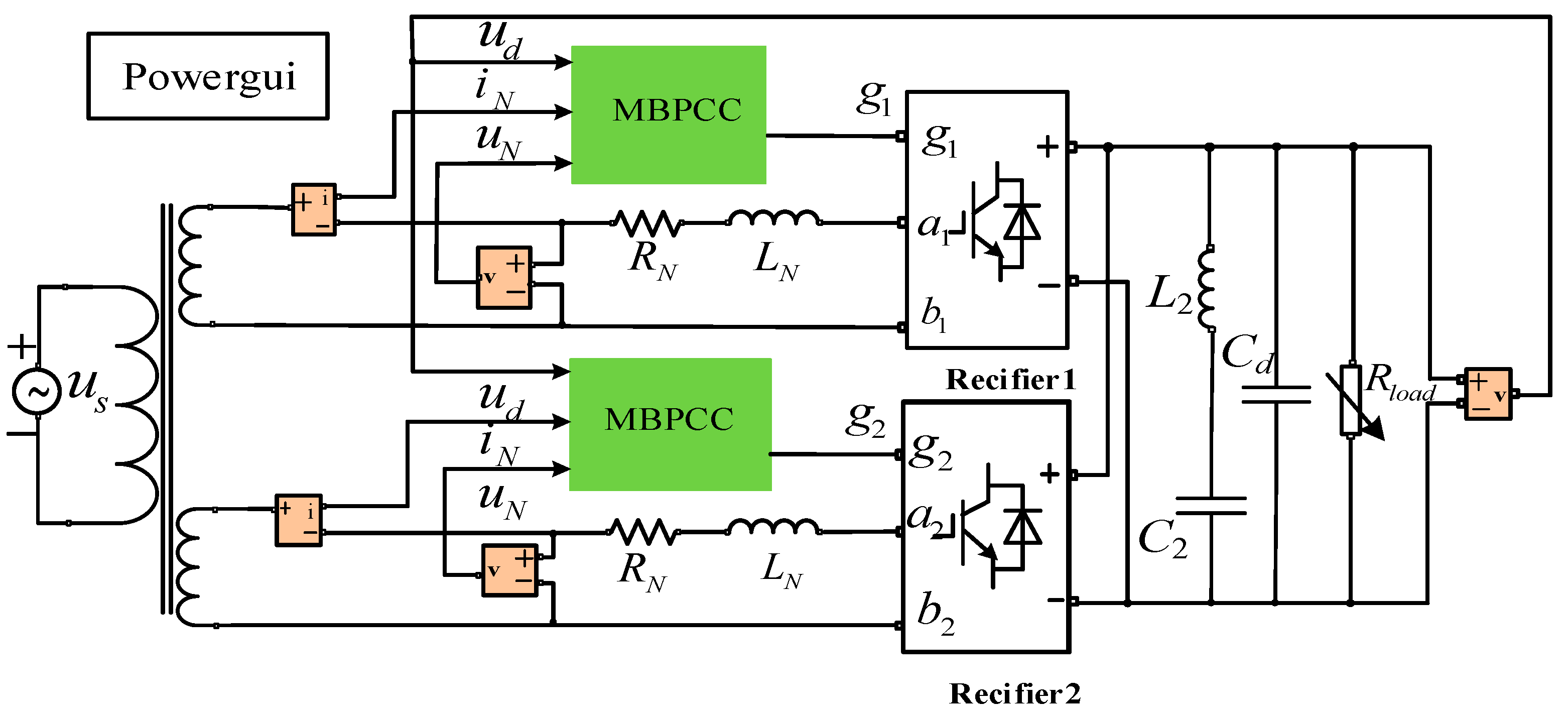
2. Model Predictive Control of One Traction Line-Side Converter of China Railway High-Speed 3 Electric Multiple Units

2.1. Mathematical Model of One Traction Line-Side Converter

The vehicle-grid coupling system of high-speed railway is composed of the traction network and the EMUs traction drive system, as shown in Figure 2. In this paper, a CRH3 EMU is set as the study object; thus, the topology of the traction drive unit of EMUs is a single-phase two-level structure. When the LFO happens, the EMUs just start up and only supply power for the auxiliary facility by DC-side voltage. Therefore, the inverter and motor can be regarded as a pure resistance, and only part of the rectifier is involved in the equivalent circuit of one traction LSC.

In the equivalent circuit of EMUs’ traction LSC, $L_N$ and $R_N$ denote the leakage inductance and leakage resistance of the secondary winding of the vehicle transformer in EMUs, respectively. Four IGBTs ($S_1$, $S_2$, $S_3$, and $S_4$) are used to construct the two-level topology, $C_d$ is the DC-side capacitor, inductance $L_2$ and capacitor $C_2$ compose the second-order filter circuit, and the inverter and motor are replaced by a pure resistive load $R_{load}$.

According to the Kirchhoff voltage law, the relationship between the voltage and current in the AC-side is listed below:

$$u_{ab}=u_N-R_N{i}_N-L_N\frac{d{i}_N}{dt}$$

(1)

where $u_N$, $i_N$, and $u_{ab}$ represent the line voltage, line current, and input voltage of the converter, respectively. If the harmonics are neglected, $u_N$, $i_N$, and $u_{ab}$ in the dq reference frame are defined as follows:

$$\{\begin{array}{c}{u}_N=u_{Nd}\sin (\omega t)+u_{Nq}\cos (\omega t)\\ i_N=i_{Nd}\sin (\omega t)+i_{Nq}\cos (\omega t)\\ u_{ab}=u_{abd}\sin (\omega t)+u_{abq}\cos (\omega t)\end{array}$$

(2)

where $u_{Nd}$, $i_{Nd}$, and $u_{abd}$ are the d-axis components of $u_N$, $i_N$ and $u_{ab}$. $u_{Nq}$, $i_{Nq}$, and $u_{abq}$ are the q-axis components of $u_N$, $i_N$, and $u_{ab}$, respectively.

Substituting Equation (2) into Equation (1), the mathematical model of one traction LSC can be described as:

$$\{\begin{array}{c}{u}_{abd}=u_{Nd}-R_N{i}_{Nd}-L_N\frac{d{i}_{Nd}}{dt}+\omega L_N{i}_{Nq}\\ u_{abq}=u_{Nq}-R_N{i}_{Nq}-L_N\frac{d{i}_{Nq}}{dt}-\omega L_N{i}_{Nd}\end{array}$$

(3)

2.2. Model Predictive Control of One Traction Line-Side Converter

2.2.1. Predictive Model of One Traction Line-Side Converter

Applying the first-order discrete approximation to the mathematical model expressed in Equation (3), a discrete dynamic model of one traction LSC in the dq reference frame is depicted by Equation (4):

$$\{\begin{array}{c}{u}_{abd}(k)=u_{Nd}(k)-R_N{i}_{Nd}(k)-\frac{L_N}{T_s}(i_{Nd}(k+1)-i_{Nd}(k))+\omega L_N{i}_{Nq}(k)\\ u_{abq}(k)=u_{Nq}(k)-R_N{i}_{Nq}(k)-\frac{L_N}{T_s}(i_{Nq}(k+1)-i_{Nq}(k))-\omega L_N{i}_{Nd}(k)\end{array}$$

(4)

where $T_s$ is the sampling interval. $i_{Nd}(k)$ and $i_{Nq}(k)$ are the discrete values of $i_{Nd}$ and $i_{Nq}$, respectively; $i_{Nd}(k+1)$ and $i_{Nq}(k+1)$ are the one-step predictive discrete values of $i_{Nd}$ and $i_{Nq}$, respectively; and $u_{abd}(k)$ and $u_{abq}(k)$ are the discrete values of the control voltages at the k-th sampling instant.

Thus, $i_{Nd}(k+1)$ and $i_{Nq}(k+1)$ can be predicted at the k-th sampling instant:

$$\{\begin{array}{c}{i}_{Nd}(k+1)=(1-\frac{T_s{R}_N}{L_N})i_{Nd}(k)+T_s\omega i_{Nq}(k)-\frac{T_s}{L_N}{u}_{abd}(k)+\frac{T_s}{L_N}{u}_{Nd}(k)\\ i_{Nq}(k+1)=(1-\frac{T_s{R}_N}{L_N})i_{Nq}(k)-T_s\omega i_{Nd}(k)-\frac{T_s}{L_N}{u}_{abq}(k)+\frac{T_s}{L_N}{u}_{Nq}(k)\end{array}$$

(5)

The relationship between $u_{ab}(k)$ and $u_{ab}(k-1)$ is satisfied in the following way:

$$\{\begin{array}{c}{u}_{abd}(k)=u_{abd}(k-1)+\Delta u_{abd}(k)\\ u_{abq}(k)=u_{abq}(k-1)+\Delta u_{abq}(k)\end{array}$$

(6)

where $\Delta u_{abd}(k)$ represents the variation between $u_{abd}(k)$ and $u_{abd}(k-1)$, and $\Delta u_{abq}(k)$ represents the variation between $u_{abq}(k)$ and $u_{abq}(k-1)$.

Substituting Equation (6) into Equation (5), then:

$$\{\begin{array}{c}{i}_{Nd}(k+1)=(1-\frac{T_s{R}_N}{L_N})i_{Nd}(k)+T_s\omega i_{Nq}(k)-\frac{T_s}{L_N}{u}_{abd}(k-1)+\frac{T_s}{L_N}{u}_{Nd}(k)-\frac{T_s}{L_N}\Delta u_{abd}(k)\\ i_{Nq}(k+1)=(1-\frac{T_s{R}_N}{L_N})i_{Nq}(k)-T_s\omega i_{Nd}(k)-\frac{T_s}{L_N}{u}_{abq}(k-1)+\frac{T_s}{L_N}{u}_{Nq}(k)-\frac{T_s}{L_N}\Delta u_{abq}(k)\end{array}$$

(7)

Equation (7) is the prediction model. It should be noted that prediction line current values are decided by present currents, voltages, and the LSC’s system parameters.

2.2.2. The Two-Step Prediction

In the digital control system, both the computation time delay and sampling time delay surely exist [28]. Because of the restriction of the hardware and the digital control algorithm, the control voltages calculated by the sampling and predictive currents have to be adopted at the (k + 1)-th sampling instant. Therefore, there is one sampling period delay ($T_d$) between the calculated control voltage by the controller and the real adopted control voltage, as shown in Figure 3. To eliminate the error caused by $T_d$, a two-step current prediction is adopted.

When two-step prediction is adopted, $i_{Nd}(k+1)$ and $i_{Nq}(k+1)$ are first predicted at the k-th sampling instant according to Equation (8), and then $i_{Nd}(k+2)$ and $i_{Nq}(k+2)$ are predicted according to Equation (9). Thus, the control voltage $u_{abd}(k+1)$ and $u_{abq}(k+1)$ can be calculated at the k-th sampling instant, and then adopted to the rectifier at the k+1-th sampling instant. The delay error is compensated by two-step prediction.

It is worth noting that $i_{Nd}(k+1)$ and $i_{Nq}(k+1)$ are also predicted through two-step prediction at the (k − 1)-th sampling instant. Thus, $i_{Nd}(k+1)$ and $i_{Nq}(k+1)$, which are predicted at the k-th sampling instant, are considered equal to the predicted values at the k−1-th sampling instant. Thus, the control voltage variations $\Delta u_{abd}(k)$ and $\Delta u_{abq}(k)$, which exist in the Equation (7), can be set to zero. The prediction Equation (7) can be rewritten as Equation (8). While $i_{Nd}(k+2)$ and $i_{Nq}(k+2)$ are not predicted before the k-th sampling instant, it cannot be affirmed that the prediction current values are equal to the k-th actual current values. The control voltages $\Delta u_{abd}(k+1)$ and $\Delta u_{abq}(k+1)$ that determine $i_{Nd}(k+2)$ and $i_{Nq}(k+2)$, respectively, cannot be omitted in Equation (9):

$$\{\begin{array}{c}{i}_{Nd}(k+1)=(1-\frac{T_s{R}_N}{L_N})i_{Nd}(k)+T_s\omega i_{Nq}(k)-\frac{T_s}{L_N}{u}_{abd}(k-1)+\frac{T_s}{L_N}{u}_{Nd}(k)\\ i_{Nq}(k+1)=(1-\frac{T_s{R}_N}{L_N})i_{Nq}(k)-T_s\omega i_{Nd}(k)-\frac{T_s}{L_N}{u}_{abq}(k-1)+\frac{T_s}{L_N}{u}_{Nq}(k)\end{array}$$

(8)

$$\{\begin{array}{c}{i}_{Nd}(k+2)=(1-\frac{T_s{R}_N}{L_N})i_{Nd}(k+1)+T_s\omega i_{Nq}(k+1)-\frac{T_s}{L_N}{u}_{abd}(k)+\frac{T_s}{L_N}{u}_{Nd}(k+1)-\frac{T_s}{L_N}\Delta u_{abd}(k+1)\\ i_{Nq}(k+2)=(1-\frac{T_s{R}_N}{L_N})i_{Nq}(k+1)-T_s\omega i_{Nd}(k+1)-\frac{T_s}{L_N}{u}_{abq}(k)+\frac{T_s}{L_N}{u}_{Nq}(k+1)-\frac{T_s}{L_N}\Delta u_{abq}(k+1)\end{array}$$

(9)

2.2.3. The Design of Performance Function

The key to achieving MPC is to obtain the most effective control quantities by solving the performance function optimally. In this paper, the optimal control voltage would be obtained.

The performance function is composed of the predicted current components at the (k + 2)-th sampling instant and the control voltage variations, with corresponding weighting coefficients [29]. The function is defined as follows:

$$w(k)={\alpha }_1{[{i_{Nd}}^{*}(k)-i_{Nd}(k+2)]}^2+{\alpha }_2{[{i_{Nq}}^{*}(k)-i_{Nq}(k+2)]}^2+{\beta }_1\Delta u_{abd}^2(k+1)+{\beta }_2\Delta u_{abq}^2(k+1)$$

(10)

where ${\alpha }_1$, ${\alpha }_2$, ${\beta }_1$, and ${\beta }_2$ represent the weighting coefficients of the line current and voltage variations.

There are no analytical or numerical methods or control design theories to adjust these parameters; currently, they are determined based on empirical procedures. In [30], an approach based on an empirical procedure is presented to obtain suitable weighting factors. When more objectives are considered, the weighting coefficients are usually obtained using trial and error procedures and running time-consuming simulations [31]. Since the front two components in Equation (10) are both the current variables, weighting factors can be considered as the same, as are the back two components. Thus, if two of weighting coefficients are decided, the other two can also be set, which can be clearly seen from

Table A1. Parameters of EMUs’ dual traction LSCs under MBPCC.

System Parameter	Value	Control Parameter	Value
$u_s$	25 kV	$K_{iv}$	0.1
$L_N$	0.004 H	$K_{pv}$	9
$R_N$	0.06 Ω	${\alpha }_1$	1
$L_2$	0.00084 H	${\alpha }_2$	1
$C_2$	0.003 F	${\beta }_1$	0.0002
$C_d$	0.006 F	${\beta }_2$	0.0002
$U_d$	3000 V	--	--
$R_{load}$	10 Ω	--	--

.

In order to make $i_{Nd}(k+2)$ and $i_{Nq}(k+2)$ track their references $i_{Nd}{(k)}^{*}$ and $i_{Nq}{(k)}^{*}$, the variations of the control voltage need to be kept as small as possible. To do this, take the derivative of Equation (10) to find the extreme point, as shown in Equation (11):

$$\{\begin{array}{c}\frac{\partial w(k)}{\partial \Delta u_{abd}(k+1)}=0\\ \frac{\partial w(k)}{\partial \Delta u_{abq}(k+1)}=0\end{array}$$

(11)

Substituting $i_{Nd}(k+2)$ and $i_{Nq}(k+2)$ of Equation (9) and $w(k)$ of Equation (10) into Equation (11), the optimal control variables $\Delta u_{abd}(k+1)$ and $\Delta u_{abq}(k+1)$ can be derived as Equation (12). In addition, the output control voltages $u_{abd}{(k)}^{*}$ and $u_{abq}{(k)}^{*}$ can be depicted by Equation (13):

$$\{\begin{array}{c}\Delta u_{abd}(k+1)=\frac{-L_N{T}_s{\alpha }_1}{T_s^2{\alpha }_1+L_N^2{\beta }_1}\{{i_{Nd}}^{*}(k)-[(1-\frac{T_s{R}_N}{L_N})i_{Nd}(k+1)+T_s\omega i_{Nq}(k+1)-\frac{T_s}{L_N}{u}_{abd}(k)+\frac{T_s}{L_N}{u}_{Nd}(k+1)]\}\\ \Delta u_{abq}(k+1)=\frac{-L_N{T}_s{\alpha }_2}{T_s^2{\alpha }_2+L_N^2{\beta }_2}\{{i_{Nq}}^{*}(k)-[(1-\frac{T_s{R}_N}{L_N})i_{Nq}(k+1)-T_s\omega i_{Nd}(k+1)-\frac{T_s}{L_N}{u}_{abq}(k)+\frac{T_s}{L_N}{u}_{Nq}(k+1)]\}\end{array}$$

(12)

$$\{\begin{array}{c}{u}_{abd}{(k)}^{*}=u_{abd}(k+1)=u_{abd}(k)+\Delta u_{abd}(k+1)\\ u_{abq}{(k)}^{*}=u_{abq}(k+1)=u_{abq}(k)+\Delta u_{abq}(k+1)\end{array}$$

(13)

The optimal control voltages that minimize the performance function are calculated by Equation (13), and then fed to a modulator stage to generate the PWM drive signal g at the k-th instant. An MBPCC controller of LSCs can be designed based on the deducing process of prediction model, the delay compensation, and the solution of performance function. Figure 4 shows the block diagram of the MBPCC. A PI controller is adopted in the voltage loop to regulate the DC-side voltage, and its output is set as the current d-axis reference $i_{Nd}{(k)}^{*}$. In addition, the q-axis current reference $i_{Nq}{(k)}^{*}$ generally needs to equal zero to achieve the unit power factor.

When LFO happens in high-speed railways, the fluctuation of the traction network’s voltage will disturb the performance of the EMUs’ LSC. Currents and voltages of the controller cannot trace well with the references, and lead to greater deterioration of fluctuation. MBPCC is a current-controlled strategy constituted by a prediction model and the performance function. By making the performance function minimal, the optimal control variables can be calculated to ensure the prediction current value tracking the references. Therefore, it is possible to adopt MBPCC to optimize the performance of the converter controller and suppress the LFO.

3. Simulations of One Traction Drive Unit of Electric Multiple Units

To validate the feasibility and effectiveness of the proposed method, simulation verifications based on the model of EMUs’ dual traction LSCs, namely the traction drive unit, were carried out from several aspects, by comparing with the control performance of traditional TDCC in MATLAB /SIMULINK, respectively. The simulation model of EMUs’ dual traction LSCs was built as shown in Figure 5. The adjustable parameters in the TDCC and MBPCC controllers were regulated into the most appropriate values, as listed in Table A1 and

Table A2. Parameters of EMUs’ dual traction LSCs under TDCC.

System Parameter	Value	Control Parameter	Value
$u_s$	25 kV	$K_{iv}$	0.1
$L_N$	0.004 H	$K_{pv}$	9
$R_N$	0.06 Ω	G	1
$L_2$	0.00084 H	--	--
$C_2$	0.003 F	--	--
$C_d$	0.006 F	--	--
$U_d$	3000 V	--	--
$R_{load}$	10 Ω	--	--

.

The block diagram of TDCC is shown in Figure 6. The outer voltage control loop uses a PI controller to keep the DC-side voltage equal to its reference value, and the PI output provides the reference of input current. The proportional controller of the inner current control loop makes the input current track its reference value.

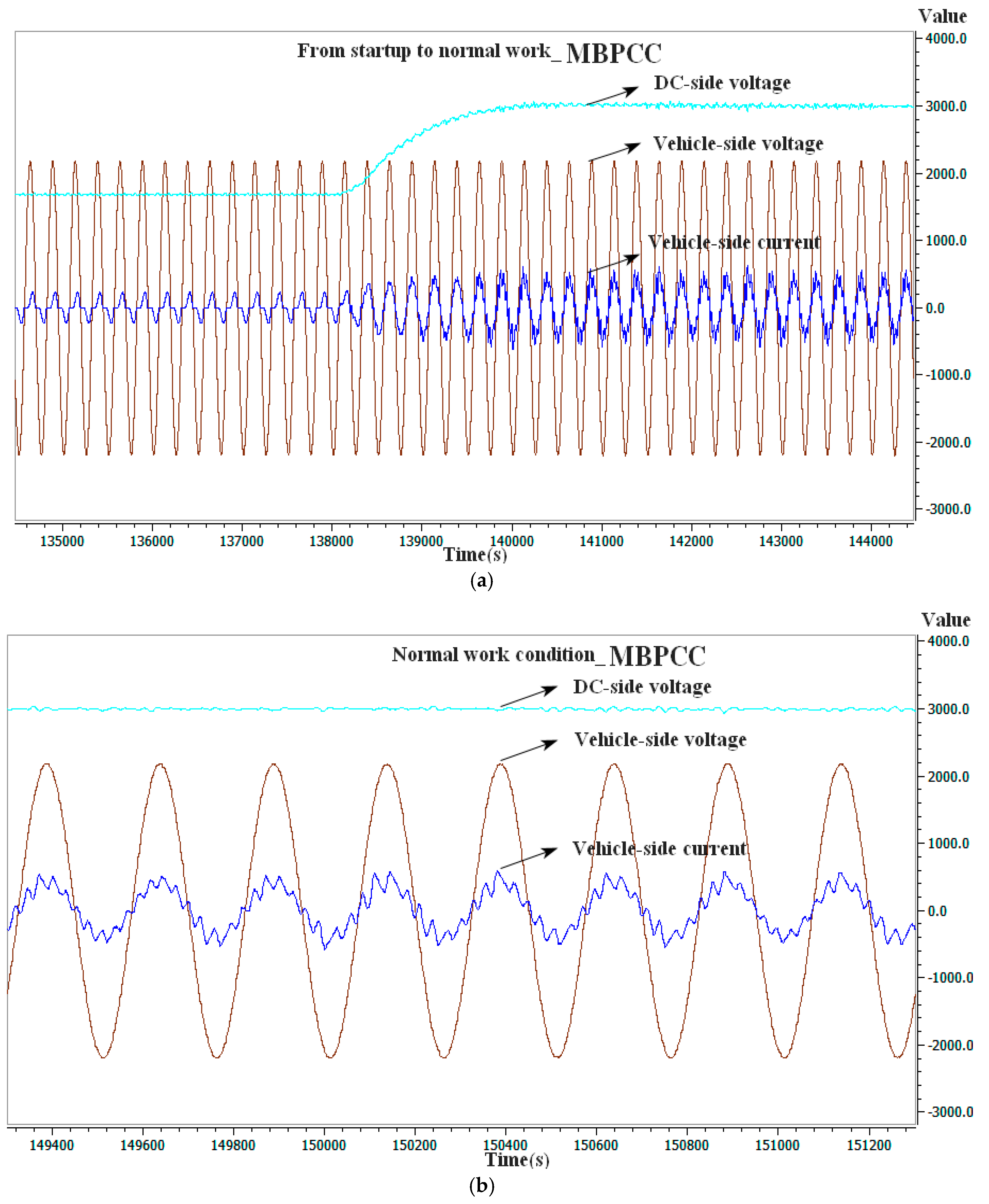
3.1. Start-Operation Process

The start-operation process of EMUs’ dual traction LSCs is divided into three periods—namely, the pre-charge period, the uncontrolled rectifier period, and the nominal load period. In the simulation, the initial time of the three stages was set to 0 s, 0.2 s, and 0.4 s, respectively. To compare MBPCC with TDCC, the waveforms of $u_N$ and $i_N$, as well as $u_d$ are depicted in Figure 7. The performance indexes of the $u_d$ of EMUs’ dual traction LSCs are shown in

Table 1. Comparison of performance indexes.

Control	Overshoot	Peak Time	Adjustment Time	Voltage Fluctuation
MBPCC	3.33%	0.10 s	0.25 s	±10 V
TDCC	26.70%	0.12 s	0.40 s	±40 V

. Figure 8 shows the fast Fourier transform (FFT) analysis results of the $i_N$ with MBPCC and TDCC.

In Figure 7, the pre-charge and uncontrolled rectifier periods of TDCC are almost the same as MBPCC’s. When the nominal load is accessed, the $u_d$ based on TDCC achieves the reference value after 0.4 s, with a large overshoot. However, the $u_d$ based on MBPCC achieves stability after 0.25 s, and the overshoot is about 100 V, far less than that of the PI control. The voltage fluctuation range of MBPCC is only ±10 V, while the voltage fluctuation based on TDCC is larger. In Figure 8, the total harmonic distortion (THD) of $i_N$ based on MBPCC is 4.76%, apparently lower than that of TDCC. In the control system based on MBPCC, there are more high-order harmonics around the odd switching frequency, which is considered as a drawback of the control strategy. Overall, MBPCC presents a better performance and dynamic response, due to the smaller overshoot, shorter adjustment time, and tinier voltage fluctuation.

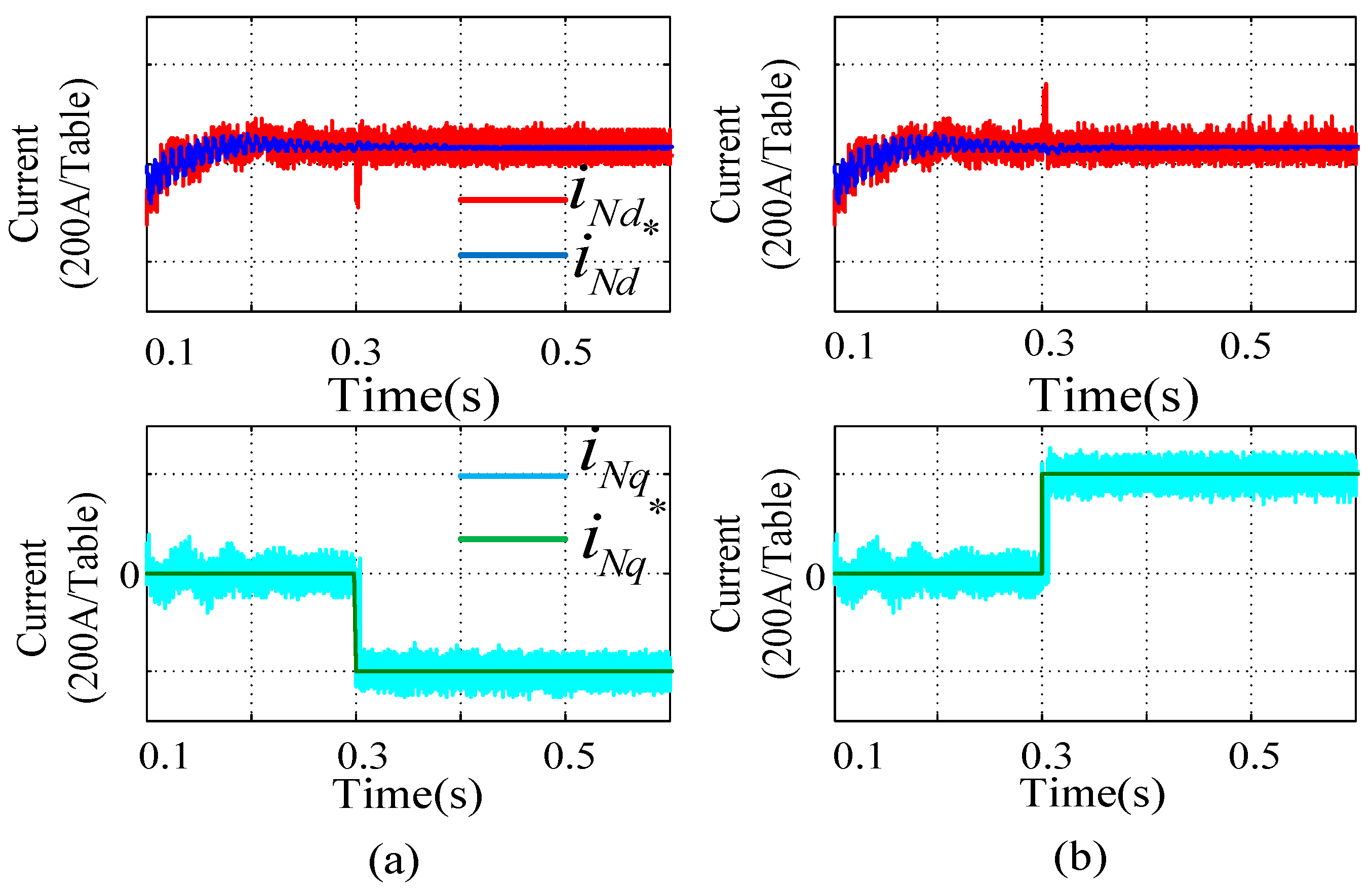
3.2. Sudden-Load-Change Process

To further validate the dynamic response performance, the simulations under the sudden-load-change condition were carried out. Figure 9 shows the simulation waveforms of the dynamic response of the $u_d$ under the condition of the load changing suddenly, based on MBPCC and TDCC, respectively. The load changes at 1 s, from 10 Ω to 0.01 Ω. Based on MBPCC, the $u_d$ has gone through a period of voltage decline from 3000 V to about 2500 V, and returns to 3000 V after 0.5 s, with a ±20 V voltage fluctuation later. In contrast, the $u_d$ based on TDCC drops by nearly 800 V, and fluctuates in the range of ±50 V after becoming stable again. Therefore, it can be concluded that the MBPCC has a better capacity for resisting disturbance than the transient PI control, because of smaller voltage decline and fluctuation when the load changes suddenly.

3.3. Track Performance

At first, we measured ${i_{Nd}}^{*}$ when the outer voltage loop plays a role in obtaining the reference current value. ${i_{Nd}}^{*}$ was about equal to 830 A, and ${i_{Nq}}^{*}$ was set to zero. Based on the measured values, we replaced the outer voltage loop by a step signal, to test the track performance while the reference current steps up or down similarly, a step signal replaces the constant module, in order to detect the track performance while the reference current ${i_{Nq}}^{*}$ steps up or down.

As shown in Figure 10a, $i_{Nd}$ decreased with ${i_{Nd}}^{*}$, varying from 830 A to 600 A at 0.3 s, and $i_{Nq}$ returned to zero after a prompt downward fluctuation. In Figure 10b, $i_{Nd}$ increases, with ${i_{Nd}}^{*}$ varying from 830 A to 1000 A, and $i_{Nq}$ rapidly returns the setting value ${i_{Nq}}^{*}$ after an upward shock. Similar conditions can be seen in Figure 11, when ${i_{Nq}}^{*}$ varies. In two cases, $i_{Nd}$ and $i_{Nq}$ can quickly track the reference current values of ${i_{Nd}}^{*}$ and ${i_{Nq}}^{*}$ in a very short time, regardless of whether ${i_{Nd}}^{*}$ or ${i_{Nq}}^{*}$ steps up or down. Thus, MBPCC could guarantee that the system has good track performance when the reference current value changes.

In conclusion, MBPCC presents a better control performance for EMUs’ dual traction LSCs, due to the smaller overshoot, shorter adjustment time, and tinier voltage fluctuation in the start-operation process, as well as its greater capacity for resisting disturbance and better track performance between the actual current and the reference current.

4. Semi-Physical Test of Electric Multiple Units’ Dual Traction Line-Side Converter

To reflect the real application condition, a whole dSPACE semi-physical experimental platform was established. The dSPACE semi-physical experimental platform included the dSPACE simulator, the physical control circuit chassis, a power supply, and an external PC, as shown in Figure 12. The dSPACE simulator was used to simulate the circuit topology of EMUs’ dual traction LSCs, and connected with the PC through a network line, so as to import the circuit simulation model from the PC to the dSPACE simulator. The physical control circuit chassis was connected to the PC through the data cable, in order to achieve the control algorithm program import and debugging. The power supply was supplied to the physical control circuit chassis.

The most important part of the dSPACE semi-physical experimental platform was the physical control circuit chassis, which was composed of the main five modules, as shown in right-hand section of Figure 12:

(1)

Switching power supply module: the switching power supply module has the function of a power supply for the entire physical control circuit chassis.

(2)

SMC module: the SMC module realizes the data transmission of the physical control circuit chassis and the outside. After control program is compiled on the computer, the SMC module achieves the connection with the computer through the data cable, and control strategy is imported into the physical control circuit chassis.

(3)

LCC module: an LCC module contains four internal DSPs, each of which controls a single converter. A physical control circuit chassis contains three LCC modules, so it can control six dual traction LSCs.

(4)

APA module: the dSPACE simulation voltage and current signals are transmitted to the APA module through the analog signal channel, and the module achieves the signal acquisition of the physical control circuit chassis.

(5)

Pulse conversion module: the pulse conversion module outputs the digital control signal of EMUs; thus, it can realize the control for EMUs directly.

Figure 13 and Figure 14 show the simulation waveforms of $u_N$ and $i_N$, as well as $u_d$ when the system of dual traction LSCs are tested on the dSPACE semi-physical platform using MBPCC and TDCC, respectively. The numerical value on the abscissa multiplied by $8{\mathrm{e}}^{-5}$ represents the simulation time. The process is performed from startup to normal working conditions.

The experimental results on the dSPACE semi-physical platform are almost in accordance with the simulation results in MATLAB. In Figure 13a, the $u_d$ based on MPBCC achieves the reference value without the overshoot. As seen in Figure 13b, $i_N$ can remain in phase with $u_N$, which means that the dual traction LSCs operate with a unified power factor. Compared with TDCC, as shown in Figure 14, $i_N$ based on MBPCC has the smaller harmonic distortion.

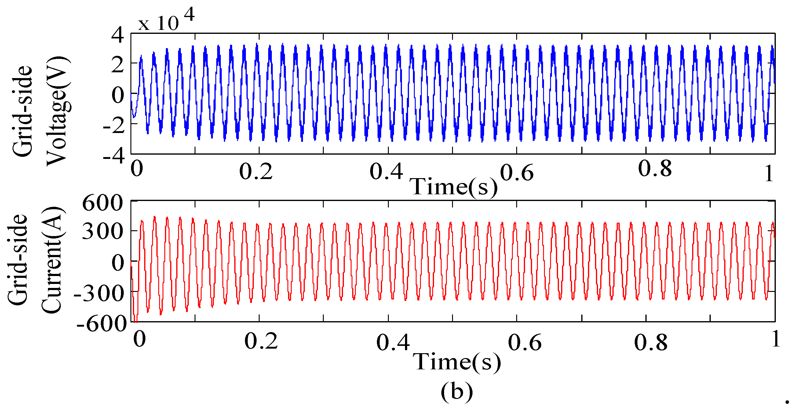
5. System Verification

The dSPACE semi-physical experiment when multi-EMUs are accessed in the power supply system is still a challenge. To verify the suppression effect of LFO and perform further sensibility analyses, the simulations of seven EMUs accessed in traction network were performed in MATLAB/SIMULINK. The autotransformer power supply system is mostly adopted in high-speed railways of China. The structure of a traction network is very complicated because of a mass of multi-conductor transmission lines that are distributed, as well as the mutual coupling effect [5]. Therefore, considering the practical factors, such as the skin effect of lines and external disturbances, it is more reasonable to adopt a reduced-order method to model the traction network [5,32] than the Thevenin-equivalent method used in [33]. Avoiding a duplication of effort, the modeling process of the vehicle-grid coupling system is no longer described.

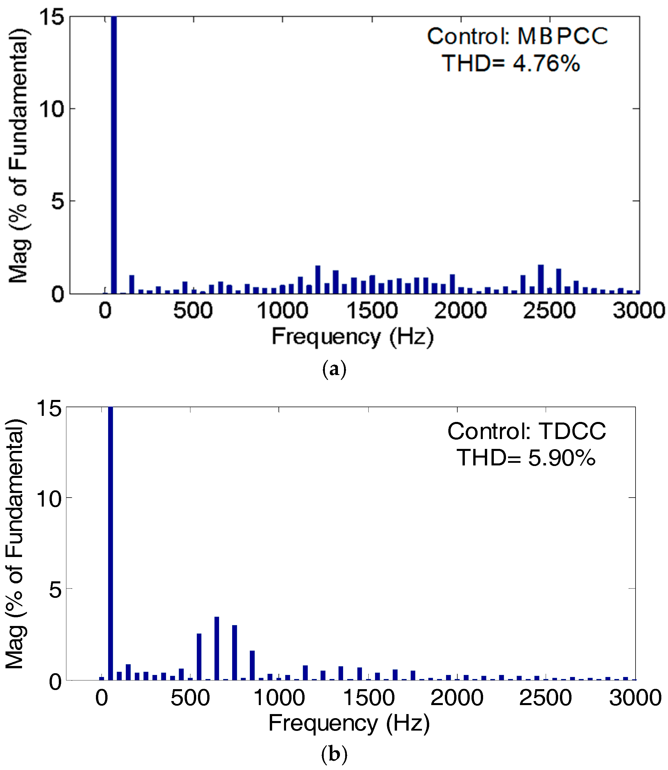
5.1. The Effect of Suppressing Low-Frequency Oscillation

Based on the TDCC controller, when seven vehicles are accessed in the reduced-order model of traction network, LFO occurs in both voltage and current, as shown in Figure 15. The $u_d$ fluctuates between 2600 V and 3600 V. It can also be found that the traction network voltage arrives at the wave crest while the grid-side current reaches the wave trough. The amplitude fluctuation of voltages and currents will influence the performance of the EMUs’ LSC, and even lead to a traction blockade.

By adopting the proposed MBPCC strategy, the system can still achieve stability when the number of multi-EMUs accessed in the traction network reaches seven. Figure 16 shows the simulation results when seven EMUs are accessed. It can be observed that the LFO does not appear even though vehicle numbers have reached their critical value. In a stable state, the $u_d$ remains stable at about 3000 V, and the voltage deviation is ±10 V. The fluctuations of grid-side voltage and current are small.

5.2. Analysis of System Parameters

The analysis of parameter sensitivity is necessary to find out their influence on the stability of the vehicle-grid coupling system. In this paper, in order to find out the effects of different external parameters on the LFO and the performance of traction LSC, three parameters (the load resistance $R_{load}$, equivalent leakage inductance, $L_N$ and the distance to power supply D) are discussed when seven vehicles are accessed in the traction network.

5.2.1. Load Resistance $R_{load}$

Figure 17 shows the waveforms of the $u_d$ under TDCC and MBPCC, when the load resistance $R_{load}$ is set as 20, 50, 75, or 100 Ω, respectively. As seen in

Table 2. Performance of the system.

Item	Value	TDCC		MBPCC
		Oscillation Pattern	Oscillation Peak (V)	Overshoot (V)	Regulation Time (s)
$R_{load}$ (Ω)	20	Stable	3600	3200	0.25
	50	Damping	[3500, 3350]	3200	0.25
	75	No	-	3200	0.25
	100	No	-	3200	0.25
$L_N$ (H)	0.001	No	-	3200	0.25
	0.002	Damping	[3500, 3350]	3200	0.25
	0.004	Stable	3600	3200	0.25
	0.006	Stable	3700	3200	0.25
$D$ (km)	10	Damping	[3240, 3530]	3200	0.20
	20	Damping	[3240, 3520]	3200	0.20
	30	Damping	[3300, 3520]	3200	0.30
	40	Stable	3500	3300	0.50

(1) Damping oscillation: the oscillation peak diminishes gradually and returns final to a stable state; (2) Stable oscillation: the oscillation peak abidingly maintains a value [9].

and Figure 17, when the load resistance $R_{load}$ varies, both the overshoot and adjustment time of the $u_d$ under MBPCC have only some tiny variations.

However, LFO happens under TDCC when the load resistance is small. The smaller $R_{load}$ is, the severer the oscillation is. LFO would not occur once $R_{load}$ exceeds a value about 75 Ω. Therefore, it can be concluded that the load resistance has fewer effects on the proposed method than TDCC.

5.2.2. Equivalent Leakage Inductance $L_N$

In Figure 18, when the equivalent leakage inductance of vehicle transformer $L_N$ varies from 0.001 H to 0.006 H, the system under MBPCC maintains an initially good dynamic performance, with little change in the $u_d$’s overshoot and regulation time. Hence, MBPCC can keep good performance and be unaffected by the change of $L_N$, while TDCC is very sensitive. When $L_N$ is set as 0.001 H, the LFO does not happen. With the increase of $L_N$, oscillation appears, and the oscillation peak enlarges gradually.

5.2.3. Distance to Power Supply D

D represents the distance to the power supply in the traction network. The larger D is, the larger the equivalent impedance on the line side will be. As seen in Figure 19 and Table 2, with the change of D, the influence on MBPCC’s control performance is slight, because the overshoot and adjustment time change only slightly more than before, and the LFO does not happen.

As for TDCC, the oscillation phenomenon can be observed when D was chosen as 10, 20, 30, and 40 km. The oscillation peak value is about 3500 V at first, and then gradually diminishes in the former three cases; when D is 40 km, the oscillation peak will be kept at 3500 V. The details are listed in Table 2. It was found that the oscillation peak varies from 3530 V to 3240 V within 1 s when D is 10 km, and from 3520 V to 3300 V when D is 30 km. The damping capability of LFO decreases with the increase of D under TDCC.

Contrasting results show that MBPCC can be almost unaffected by the three parameters, and LFO does not happen when these parameters change. However, the performance of TDCC is sensitive to the three parameters. Both the oscillation pattern and oscillation peak can be easily influenced when the parameters change.

6. Conclusions

To optimize the control performance of EMUs’ traction drive units, namely dual traction LSCs, and suppress LFO in vehicle-grid coupling system of high-speed railways, MBPCC is proposed in order to apply the traction LSC of CRH3 EMUs. After theoretical analysis, simulation verifications, and semi-physical verifications, the performance of MBPCC is demonstrated in comparison to TDCC, and the advantages of each listed below:

(1)

Simulation verifications in MATLAB of EMUs’ dual traction LSCs based on MBPCC and TDCC were implemented from three aspects. The results prove that MBPCC can obtain better dynamic and static performances, such as a smaller THD, tinier overshoot in start-operation process, greater capacity for resisting disturbance under load changing suddenly, and a better track performance.

(2)

Semi-physical verifications in the dSPACE semi-physical experimental platform were realized. The results certified the effectiveness of MBPCC and its superiority in real applications, when compared with TDCC.

(3)

When the multi-EMUs were assessed in the reduced-order model of traction network, the results showed that MBPCC can ensure the system’s stability and suppress LFO more efficiently compared with TDCC.

(4)

The influences of different external parameters $R_{load}$, $L_N$, and D in the vehicle-grid coupling system under MBPCC and TDCC have been discussed in detail. It could be concluded that these three parameters have a tiny impact on MBPCC, while they greatly influence the performance of TDCC. Both the oscillation pattern and oscillation peak under TDCC can be easily influenced when parameters change.

The proposed method can be applied for the control of EMUs’ traction LSCs, and provide a good effect on the suppression of LFO. Moreover, MBPCC is insensitive to system parameters, which provides greater possibilities for its application. There is some advanced work regarding MBPCC that can be studied in the future. In the aspect of physical verification, multi-EMUs accessed in the model of the traction network should be realized in order to increase the reliability for suppressing LFO. With respect to algorithm optimization, combining predictive control with the disturbance observer can further advance the performance and robustness of the system, which can deal with the modeling errors and uncertainties, disturbances, and sensor noise.

References

1. Menth, S.; Meyer, M. Low frequency power oscillation in electric railway systems. EB Elektrische Bahnen 2006, 2, 216–221. [Google Scholar]
2. Eitzmann, M.; Paserba, J.; Undrill, J. Model development and stability assessment of the Amtrak 25 Hz traction system from New York to Washington DC. In Proceedings of the 1997 IEEE/ASME Joint Railroad Conference, Boston, MA, USA, 18–20 March 1997; pp. 21–28. [Google Scholar]
3. Heising, C.; Fang, J.; Bartelt, R.; Staudt, V.; Steimel, A. Modelling of rotary converter in electrical railway traction power-systems for stability analysis. In Proceedings of the Electrical Systems for Aircraft, Railway and Ship Propulsion, Bologna, Italy, 19–21 October 2010; pp. 1–6. [Google Scholar]
4. Liu, Z.; Zhang, G.; Liao, Y. Stability research of high-speed railway EMUs and traction network cascade system considering impedance matching. IEEE Trans. Ind. Appl. 2016, 5, 4315–4326. [Google Scholar] [CrossRef]
5. Zhang, G.; Liu, Z.; Yao, S.; Liao, Y.; Xiang, C. Suppression of low frequency oscillation in traction network of high-speed railway based on auto disturbance rejection control. IEEE Trans. Transp. Electrif. 2016, 2, 244–245. [Google Scholar] [CrossRef]
6. Liu, J.; Zheng, Y. Resonance mechanism between traction drive system of high-speed train and traction network. Trans. China Electro Tech. Soc. 2013, 4, 221–227. [Google Scholar]
7. Wang, H.; Wu, M. Simulation analysis on low-frequency oscillation in traction power supply system and its suppression method. Power Syst. Technol. 2015, 4, 1088–1095. [Google Scholar]
8. Heising, C.; Oettmeier, M.; Staudt, V.; Steimel, A.; Danielsen, S. Improvement of low-frequency railway power system stability using an advanced multivariable control concept. In Proceedings of the IECON, Porto, Portugal, 3–5 November 2009; pp. 560–565. [Google Scholar]
9. Danielson, S.; Fosso, O.B.; Molinas, M.; Suul, J.A.; Toftevaag, T. Simplified models of a single-phase power electronic inverter for railway power system stability analysis–development and evaluation. Electr. Power Syst. Res. 2010, 2, 204–214. [Google Scholar] [CrossRef]
10. Liao, Y.; Liu, Z.; Zhang, G.; Xiang, C. Vehicle-grid system modeling and stability analysis with forbidden region-based criterion. IEEE Trans. Power Electron. 2017, 5, 3499–3512. [Google Scholar] [CrossRef]
11. Wang, H.; Wu, M.; San, J. Analysis of low-frequency oscillation in electric railways based on small-signal modeling of vehicle-grid system in d-q frame. IEEE Trans. Power Electron. 2015, 9, 5318–5328. [Google Scholar] [CrossRef]
12. Dabra, V.; Paliwal, K.K.; Sharma, P. Optimization of photovoltaic power system: A comparative study. Prot. Control Mod. Power Syst. 2017, 2, 3. [Google Scholar] [CrossRef]
13. Liu, J.; Yang, D.; Yao, W.; Fang, R.; Zhao, H.; Wang, B. PV-based virtual synchronous generator with variable inertia to enhance power system transient stability utilizing the energy storage system. Prot. Control Mod. Power Syst. 2017, 2, 429–437. [Google Scholar] [CrossRef]
14. Agorreta, J.L.; Borrega, M.; López, J.; Marroyo, L. Modeling and control of N-paralleled grid-connected inverters with LCL filter coupled due to grid impedance in PV plants. IEEE Trans. Power Electron. 2011, 3, 770–785. [Google Scholar] [CrossRef]
15. Hernández, J.C.; De La Cruz, J.; Vidal, P.G.; Ogayar, B. Conflicts in the distribution network protection in the presence of large photovoltaic plants: The case of ENDESA. Int. Trans. Electr. Energy Syst. 2013, 5, 669–688. [Google Scholar] [CrossRef]
16. Enslin, J.H.R.; Hulshorst, W.T.J.; Atmadji, A.M.S.; Heskes, P.J.M.; Kotsopoulos, A.; Cobben, J.F.G.; Van der Sluijs, P. Harmonic interaction between large numbers of photovoltaic inverters and the distribution network. In Proceedings of the IEEE Bologna Power Tech Conference Proceedings, Bologna, Italy, 23–26 June 2003; pp. 75–80. [Google Scholar]
17. Wang, H.; Wu, M. Review of low-frequency oscillation in electric railways. Trans. China Electro Tech. Soc. 2015, 17, 70–78. [Google Scholar]
18. Cortés, P.; Kazmierkowski, M.P.; Kennel, R.M.; Quevedo, D.E.; Rodríguez, J. Predictive control in power electronics and drives. IEEE Trans. Ind. Electron. 2008, 12, 4312–4324. [Google Scholar] [CrossRef]
19. Vazquez, S.; Leon, J.I.; Franquelo, L.G.; Rodriguez, J.; Young, H.A.; Marquez, A.; Zanchetta, P. Model predictive control: A review of its applications in power electronics. IEEE Ind. Electron. Mag. 2014, 1, 16–31. [Google Scholar] [CrossRef] [Green Version]
20. Hu, J.; Cheng, K.W.E. Predictive control of power electronics converters in renewable energy systems. Energies 2017, 4, 515. [Google Scholar] [CrossRef]
21. Chan, R.; Kwak, S. Improved Finite-Control-Set Model Predictive Control for Cascaded H-Bridge Inverters. Energies 2018, 2, 355. [Google Scholar] [CrossRef]
22. Vazquez, S.; Marquez, A.; Aguilera, R.; Quevedo, D.; Leon, J.I. Predictive optimal switching sequence direct power control for grid-connected converters. IEEE Trans. Ind. Electron. 2015, 4, 2010–2020. [Google Scholar] [CrossRef]
23. Xia, C.; Liu, T.; Shi, T.; Song, Z. A simplified finite-control-set model-predictive control for power converters. IEEE Trans. Ind. Inf. 2014, 2, 991–1002. [Google Scholar]
24. Aguilera, R.P.; Lezana, P.; Quevedo, D.E. Finite-control-set model predictive control with improved steady-state performance. IEEE Trans. Ind. Inf. 2013, 2, 658–667. [Google Scholar] [CrossRef]
25. Song, W.; Ma, J.; Zhou, L.; Feng, X. Deadbeat predictive power control of single-phase three-level neutral point clamped converters using space-vector modulation for electric railway traction. IEEE Trans. Power Electron. 2016, 1, 721–732. [Google Scholar] [CrossRef]
26. Song, W.; Deng, Z.; Feng, X. A simple model predictive power control strategy for single-Phase PWM converters with modulation function optimization. IEEE Trans. Power Electron. 2016, 7, 5279–5289. [Google Scholar] [CrossRef]
27. Aguilera, R.P.; Quevedo, D.E.; Vázquez, S.; Franquelo, L.G. Generalized predictive direct power control for ac/dc converters. In Proceedings of the 2013 IEEE ECCE Asia Downunder, Melbourne, Australia, 3–6 June 2013; pp. 1215–1220. [Google Scholar]
28. Cortés, P.; Rodriguez, J.; Silva, C.; Flores, A. Delay compensation in model predictive current control of a three-phase inverter. IEEE Trans. Ind. Electron. 2012, 2, 1323–1325. [Google Scholar] [CrossRef]
29. Ma, H.; Li, Y.; Zheng, Z.; Xu, L.; Wang, K. PWM rectifier using a model predictive control method in the current loop. Trans. China Electro Tech. Soc. 2014, 8, 136–141. [Google Scholar]
30. Cortes, P.; Kouro, S.; La Rocca, B.; Vargas, R.; Rodriguez, J.; Leon, J.; Vazquez, S.; Franquelo, L. Guidelines for weighting factors design in model predictive control of power converters and drives. In Proceedings of the IEEE International Conference on Industrial Technology, Gippsland, Australia, 10–13 February 2009; pp. 1–7. [Google Scholar]
31. Zanchetta, P. Heuristic multi-objective optimization for cost function weights selection in finite states model predictive control. In Proceedings of the 2011 Workshop on Predictive Control of Electrical Drives and Power Electronics, Munich, Germany, 14–15 October 2011; pp. 70–75. [Google Scholar]
32. Leng, Y.; Yang, H.; Wang, Z. A method of suppressing low-frequency oscillation in traction network based on two-degree-of-freedom internal model control. Power Syst. Technol. 2017, 1, 258–264. [Google Scholar]
33. Lee, H.M.; Lee, C.M.; Jiang, G. Harmonic analysis of the Korean high-speed railway using the eight-port representation model. IEEE Trans. Power Deliv. 2006, 2, 979–986. [Google Scholar] [CrossRef]
Figure 1. The study idea of the article.
Energies 11 01803 g001
Figure 2. Vehicle-grid coupling system.
Energies 11 01803 g002
Figure 3. Control voltage in two switching periods.
Energies 11 01803 g003
Figure 4. Block diagram of model-based predictive current control (MBPCC).
Energies 11 01803 g004
Figure 5. The circuit of electric multiple units’ (EMUs’) dual traction line-side converters (LSCs), based on MBPCC.
Energies 11 01803 g005
Figure 6. Block diagram of transient direct current control (TDCC).
Energies 11 01803 g006
Figure 7. Simulation waveforms of u N with i N , as well as u d , using (a) MBPCC and (b) TDCC.
Energies 11 01803 g007
Figure 8. FFT results for i N under (a) MBPCC and (b) TDCC.
Energies 11 01803 g008
Figure 9. Simulation waveforms of the dynamic response of the u d when the load suddenly changes, with (a) MBPCC and (b) TDCC.
Energies 11 01803 g009
Figure 10. Simulation waveforms of i N d and i N q when (a) i N d * varies from 830 A to 600 A and when (b) i N d * varies from 830 A to 1000 A.
Energies 11 01803 g010
Figure 11. Simulation waveforms of i N d and i N q when (a) i N q * varies from 0 A to −200 A and (b) when i N q * varies from 0 A to 200 A.
Energies 11 01803 g011
Figure 12. The dSPACE semi-physical experimental platform.
Energies 11 01803 g012
Figure 13. Waveforms of u N and i N , as well as u d using MBPCC: (a) the process from startup to normal work; and (b) normal working conditions.
Energies 11 01803 g013
Figure 14. Waveforms of u N and i N , as well as u d , using TDCC (a) the process from startup to normal work and (b) under normal working conditions.
Energies 11 01803 g014
Figure 15. Waveforms of seven EMUs accessed with TDCC: (a) u d ; and (b) grid-side voltage and current.
Energies 11 01803 g015
Figure 16. Waveforms of seven EMUs accessed with MBPCC: (a) u d and (b) grid-side voltage and current.
Energies 11 01803 g016aEnergies 11 01803 g016b
Figure 17. Waveforms of u d when R l o a d = 20, 50, 75, or 100 Ω.
Energies 11 01803 g017
Figure 18. Waveforms of u d when L N = 0.001, 0.002, 0.004, and 0.006 H.
Energies 11 01803 g018
Figure 19. Waveforms of u d when D = 10, 20, 30, and 40 km.
Energies 11 01803 g019