Energy Prices, Real Estate Sales and Industrial Output in China

Abstract

A majority of energy is consumed to control the indoor environment for human activities and industrial production. The demand for energies for these two uses are reflected in demand for different types of real estate and the volume of industrial outputs. The purpose of this study is to examine the long-run equilibrium and short-run dynamics between real energy prices and demand for different types of real estate and industrial output in China. Energy prices are measured in the real price of fuels and power. Demand for different types of real estate is measured in their sales volume in the first hand market, that is, floor areas of new real estate sold by developers. Industrial output is measured by the net output (value added) of the industrial sector. All data series were tested for stationarity (i.e., the existence of a unit root) before testing for a co-integration relationship. We found no long-term equilibrium relationship between energy prices and the demand for real estate and industrial output as predicted by theory, probably due to increased supply of energy efficient buildings. There is also no short-run relationship between energy prices and demand for housing due to the increase in vacancy rate resulting from speculative demand for housing. However, demand for commercial properties appeared to lead energy prices. Finally, there is strong evidence suggesting that an increase in energy prices will significantly reduce industrial output but not vice versa.

1. Introduction

In 2015, China consumed 4.30 billion tons of coal equivalent (tce) of energy and its net imports of energy were 677 million tce [1]; China emitted 9213 million tons of carbon dioxide (CO₂), which is 67.5% more than the world’s second-largest US emissions (5445 million tons) [2].

Real estate is a sheltered space in a controlled environment for human activities. Such a controlled environment is achieved by consuming energies. Therefore, the occupation of real estate assets is a major source of energy consumption. The importance of energy consumption in different types of buildings is also reflected in government policies to promote energy-efficient buildings and implementation of lower and upper temperature limits during respectively summer and winter. Therefore, in theory, a decrease in energy prices should stimulate demand for real estate due to a reduction in the operating cost of the building.

In the real estate market that is composed of real estate demand, supply, price, economic shocks (e.g., industrial growth) and others like inflation, interest rate and energy price, interactions between these factors are much complicated. On the one hand, the short-term and long-term effects between these factors and hence their exogeneity and endogeneity can be discussed in theory; real estate prices can be endogenous or exogenous relative to the market [3]. On the other hand, investigation of those effects or the decision of exogeneity and endogeneity is an empirical issue. We suggest that energy prices are a significant fundamental in China’s overall real estate market since past findings show that its economy has heavily depended on energy consumption [4,5]. Due to informational imperfections and asymmetries between sellers and buyers in the real estate market, Real estate sales may respond to a demand shock faster than real estate prices do [6]. Real estate sales appeared to be positively related to demand, for example, [7]. To simplify our analysis of the real estate market, we focus on the interactions between different types of real estate sales and real energy prices.

We understand that changes in demand also affect transaction prices in addition to Real Estate Sales. However, the first-hand real estate market prices are relatively insensitive to market conditions in the short run as they are set by developers as listing prices, which remain unchanged for a batch of units put on sale in the first-hand market. When there is an increase in demand, new units will be sold out more quickly, which is reflected in an increase in real estate sales. After a batch of new units has been sold, developers will then change the listing prices for subsequent batches of units according to the latest market conditions. Therefore, real estate sales reflect changes in demand more quickly than transaction prices in the first-hand market. Even then, we realize that real estate sales are a not a perfect proxy for real estate demand as transaction prices will also respond to changes in demand, though not as responsive as real estate sales.

Demand for real estate cannot be easily observed. Total transaction volume is a not a good indicator as the second-hand market transactions reflect the transfer of ownership only, that is, demand from the new owner is met by the supply from the seller with no net increase in total quantity demanded. Sales in the first-hand market by the developer is a better proxy for changes in demand for real estate as it shows the how much newly produced real estate assets are absorbed by the market due to a net increase in demand. Therefore, we use the volume (in square meters of floor area) of different types of real estate sold by developers in the first-hand market (“Real Estate Sales”) as a proxy for the real estate demand. Over the past ten years, real estate development and their sales activities in China have been growing rapidly. In 2006, the sales of commodity real estate were 618.57 million square meters, of which sales of commodity housing accounted for 89.6% (554.23 million square meters). By 2016, commodity real estate sold increased to 1573.49 million square meters, of which commodity housing sales accounted for 87.4% (1375.4 million square meters). Therefore, in the past ten years, total commodity real estate sales and commodity housing sales increased by 154.4% and 148.2% respectively.

The first objective of this paper is to examine whether there is any empirical relationship between energy prices and Real Estate Sales as predicted by theory. Much research so far has been focused on how the geographical attribute of real estate [8] affects its demand. This paper examines how energy prices affect total aggregate real estate demand as a result of their impact on the operating costs of buildings. If energy prices do impact on real estate demand, the market value of individual real estate may also be affected by its energy consumption and performance, which implied that energy performance variables should be included as independent variables in the use of hedonic prices for mass appraisals [9,10].

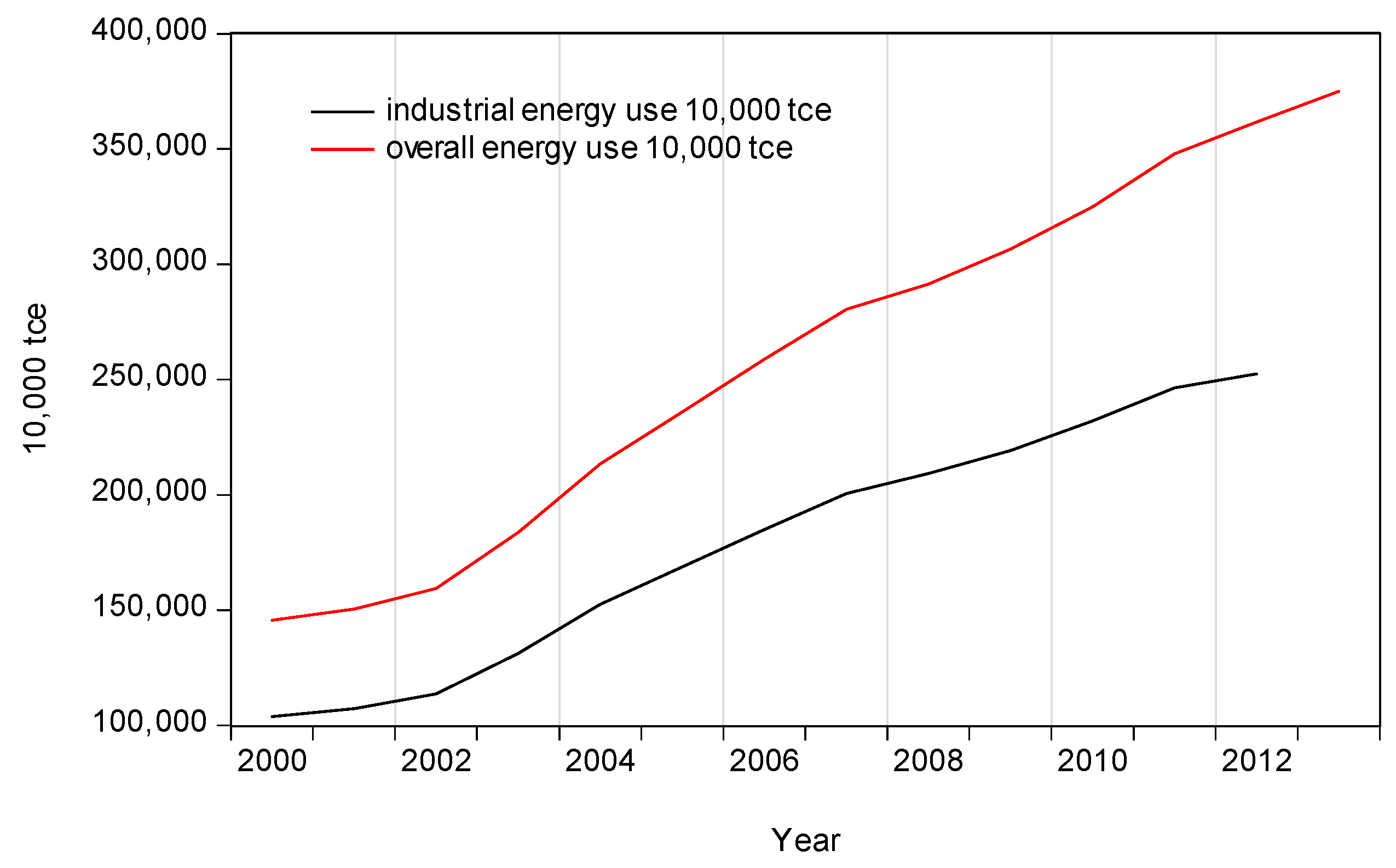
One of the major activities within the controlled environment inside a building is industrial production. As a major provider of industrial products in the world economy, China’s energy consumption in industrial production has been significant (Figure 1). The industrial sector consumed 2.92 billion tce of energy or 68.0% of the total energy consumed in 2015 [1]. Hence, we expect that there should be a significant relationship between industrial production and energy prices since energy is a major input in the industrial production process. An increase in energy prices will increase the cost of production and thus depress industrial output. The relationship between energy prices and industrial output has always been of interest to policymakers.

The remainder of this paper is organized as follows. Section 2 reviews the existing literature, while Section 3 introduces the method for empirical tests. Section 4 presents data and definitions of the variables of interest. The results of econometric analyses are presented in Section 5. Section 6 discusses the empirical results. The final section presents the conclusion.

2. Literature Review

Occupation of real estate consumes a considerable share of energy in an economy. Past studies mainly focused on the effect of energy performance on property values, which is typically evaluated by estimating the hedonic pricing model, for example, [11,12,13,14,15,16]. However, studies that examine the relationship between the energy prices and aggregate demand for real estate have been scarce. Buildings consume 41% of total U.S. energy and so represent the largest share of energy consumption in the U.S. [17]. Real estate consumes energy mainly for heating and cooling of buildings [18]. For example, space and water heating, appliances and cooking constitute 78%, 16% and 3% of British housing energy demand, respectively [19]. In China, energy consumption derived from residential accommodations accounted for 11.7% of the 2015’s overall energy consumption.

It is worth noting that energy consumption varies across real estate types. Residential real estate as a whole consumes much more energy than commercial properties since the total stock of residential buildings is larger than that of commercial and office buildings combined. However, residential buildings consumed less energy per square foot of floor area [17]. In Britain, housing property consumed energy accounted for approximately 33% of 2010’s aggregate energy demand by final consumption [20,21].

An increase in energy prices implied a higher operating cost of building and there will depress demand for new buildings (Real Estates Sales) in the long run due to increased operating costs. On the other hand, an increase in demand for real estate also implies more demand for energies and thus higher energy prices [20,21]. Real Estate Sales is a useful proxy for changes in demand for real estate, particularly for high-frequency data, for example, [7]. Studies have shown that new housing completions exert positive effects on energy prices [22] and demand for housing properties impact energy prices in the long run [23]. However real estate completion is not a good measure of demand if some completed units are not sold. Therefore, a better measure of real estate demand is Real Estate Sales.

Industry consumes a significant share of energy in China and thus a close link between energy prices and industrial output is expected. Much previous research found a negative correlation between oil prices and real output, for example, [24,25]. Past studies indicate that total industrial output for designated size enterprises in Shanghai positively impacted energy prices during the period 2006–2010. The elasticity of industrial output relative to energy prices was 0.29 [23]. The Brent oil price has negatively influenced industrial growth in Romania [26]. However, government-controlled energy prices have led to price distortions and accordingly affect the long relationship between energy prices and demand for real estate [27].

3. Methodology

This study argues that China’s real estate consumed a substantial amount of energy. Real estate sales can reflect the real estate demand [7]. Therefore, it assumes that energy prices may significantly affect the demand for real estate, which in turn affects real estate sales. Actual real estate demand often cannot be intuitively observed. Despite this, data on real estate sales are readily available. We employed real estate sales as a demand variable.

Also, the industrial sector is highly energy-intensive and dominates energy consumption. Incorporation of an industrial sector variable into the energy price-real estate economic system may be significant for system estimates and macroeconomist. Therefore, to examine the relationship between energy prices and real estate sales, the study defined an economic system vector

$$\mathbf{\Phi }=(\mathit{ENERGY}, \mathit{HOUSE}, \mathit{COMMERCIAL}, \mathit{OFFICE}, \mathit{OUTPUT})$$

(1)

where the variables in ENERGY, HOUSE, COMMERCIAL, OFFICE and OUTPUT denote real energy price, sales of new housing property, office property, commercial property and value added of the industrial sector respectively.

Cointegration theory takes all the variables in $\mathbf{\Phi }$ as endogenous a priori. Because common or similar fundamentals link these variables, the variables may move forward around a long-run equilibrium vector [28]. We tested for cointegration using the Phillips-Oularis test [29] and the Johansen trace test [30,31]. These two tests can complement each other; the Phillips-Ouliaris test can quickly provide a clue to cointegration. This test is residual-based and should have superior power properties in small samples [29]. Finite-sample critical values have been computed [32]. Nonetheless, the Johansen multivariate trace test may detect the cointegrating vector, which suggests long-term and short-term effects between variables. The cointegrating vector is also required for construction of a linear error-correction model (ECM). The trace test is based upon

$$\Delta y_t=\mathbf{\Pi }{y}_{t-1}+{\displaystyle \sum _{i=1}^{p-1}{\mathbf{\Gamma }}_i\Delta y_{t-i}+\mathbf{B}{x}_t+{\epsilon }_t}$$

(2)

where $\mathbf{\Pi }={\displaystyle {\sum }_{i=1}^p{\mathbf{A}}_i-I}$ and ${\mathbf{\Gamma }}_i={\displaystyle {\sum }_{j=i+1}^p{\mathbf{A}}_j}$. y_t is a k-vector of I(1) variables, x_t is a d-vector of deterministic variables and ε_t is a vector of white noises with zero mean and finite variance. Furthermore, $\mathbf{\Pi }=\mathit{\alpha }{\mathit{\beta }}^{\prime }$, where β and α are the cointegrating vector and corresponding adjustment coefficient, respectively. β represents the long-run relationship between time series.

Cointegration implies an error correction mechanism (ECM) for the I(1) variable set, which can lead to optimal inferences [33]. However, a first-differenced log-linear vector-autoregression (FDVAR) model is still valid for the I(1) but not the cointegrated variable set [28].

We first tested for a unit root using the augmented Dickey-Fuller (ADF) and Phillips-Perron (PP) tests [34,35]. The ADF test is based on an autoregressive specification. The PP test is nonparametric. Hence, these two tests complement each other. The standard ADF test may suffer from the power loss as well as severe size distortions and accordingly lead to over-rejection of the unit root hypothesis. On the other hand, the PP test suffers from severe size distortions [36,37]. Hence, the Elliott-Rothenberg-Stock test modifies the Dickey-Fuller test (ERS DF) and could work well in small samples [38]; notably, if this test applies the Generalized Least Squares (GLS) method to detrend data and selects the lag length using a modified AIC (MAIC), the test can report the good power and size [37]. We applied the ERS DF test along with the MAIC (The ERS DF-GLS test).

However, a breakpoint in the data likely produces incorrect inferences for unit roots [39]. A test was conducted for break-date using the Perron test in Model C [40]. Model C is recommended when the break date is taken as unknown [41]. The Perron test Model C is [39,40]

$$y_t=\mu +\theta D{U}_t+\beta t+\gamma D{T}_t+\delta D{(TB)}_t+\alpha y_{t-1}+{\displaystyle \sum _{i=1}^k{c}_i\Delta y_{t-i}}+{\epsilon }_t$$

(3)

where DU = 1 if t > T_b and 0 otherwise; DT = t − T_b if t > T_b and 0 otherwise; and D(TB) = 1 if t = T_b + 1 and 0 otherwise with 1(.) the indicator function. T is the sample. T_b is the break date. Under the null hypothesis of a unit root, $\mu \ne 0$ (in general), $\theta =0$ (except in Model C), $\beta =0$, $\gamma =0$, $\delta \ne 0$ and $\alpha =1$. Under the alternative hypothesis of stationary fluctuations around a deterministic trend function, $\mu \ne 0$, $\theta =0$, $\beta =0$, $\gamma =0$ (in general), $\delta \ne 0$ and $\alpha <1$.

4. Data

Data on monthly changes in square meters of existing real estate and the number of units are not available. Despite this, data on monthly real estate sales (turnover) in square meters are available [42].

We collected real estate sales data from the NBSC [43]. There are different commodity real estate sales area statistics between the pre-August 2005 period and the September 2008 to December 2014 period. Before August 2005, the commodity real estate sales area data were the actual square meters sold. However, that monthly sales series is available only for months after February 2005. After September 2005, the commodity real estate sales area includes two components, that is, the actual square meters sold in the current month and the square meters presold. We cannot use the presale series because the transactions for the presales may or may not be completed in the future, implying that in both cases, the presold real estate does not currently consume any energy and thereby does not influence current energy prices. To be in line with the statistics, we did not collect observations in 2005 but employed the monthly series for the period from January 2006 to December 2014. There were 108 monthly observations available for each series.

Square meter data on real estate sales were estimated from January onwards. January values were missing; therefore, we approximated January values by dividing February values by two.

Energy prices used in this study are referenced to index changes in the purchase price of fuels and power (PPFP), PPFP is measured by the nominal index change compared with the same month of the previous year. PPFP is a part of the industrial producers purchase price and reflects changes in the prices of representative energy products that selected companies purchase. Representative energy products comprise coal, gasoline, diesel, kerosene, natural gas, fuel oil, etc. In terms of use, fuel oil is used by large low-speed internal combustion ship engines, while furnace fuel oil (heavy oil) is used for a variety of industrial furnaces or boilers [44]. Since March 2009, China has adopted an oil product pricing system by which domestic oil product prices adjust to international crude oil markets. However, we find that overall energy prices are related more closely to retail fuel prices than to wholesale prices. International crude oil prices are scarcely a determinant of China’s energy prices; consider Shanghai as an example. Since April 2011, Shanghai retail gasoline prices decreased at a much slower pace than the international market. During the March 2009 to March 2014 period, the correlation coefficients between the wholesale prices of gasoline and diesel in Shanghai and the WTI crude oil futures price are 0.84 and 0.89, respectively. The Shanghai wholesale petrol and diesel prices appear to move with WTI crude oil futures prices [45,46]. Nevertheless, during the April 2009 to April 2011 period, when the WTI crude oil futures price increased by 120%, Shanghai’s average regular-grade No. 92 retail gasoline price rose 50% [47]. During the April 2011 to June 2014 period, changes in WTI crude oil futures and Shanghai gasoline prices were −7.5% and 0.26%, respectively. During the June to October 2014 period, the change in WTI crude oil and Shanghai gasoline prices were −19.8% and −5.1%, respectively.

Data on monthly changes in the price of all primary energy types (crude oil, coal, natural gas, nuclear energy, etc.) are not available. Despite this, the PPFP Index represents the cost of using electricity and a basket of selected fuels. Hence, we used the PPFP index to represent the energy price (ENERGY). We adjusted energy price indices by dividing the nominal price index by a corresponding national average monthly CPI value, resulting in prices stated in real terms. For the G-7 countries except for Japan and the U.K., oil prices have a long-run influence on the inflation rate [48]. On the contrary, there may be a causal link from higher energy prices to inflation [49].

Industrial value added (IVA) in the current month represents the industrial output (OUTPUT). January values on IVA were missing from the original data; therefore, the January value was approximated using the average of the values from the December before and February after.

We seasonally adjusted the original data utilizing the X12 (multiplicative) [50].

Table 1. Descriptive statistics of the data.

Variable	ENERGY	HOUSE	COMMERCIAL	OFFICE	OUTPUT
Definition	Fuels and power price index (same month of previous year = 100) divided by CPI	Sales of housing real estate onwards from January (10,000 square meters)	Sales of commercial real estate onwards from January (10,000 square meters)	Sales of office real estate onwards from January (10,000 square meters)	Industrial value added onwards from January (RMB 100 million)
Mean	1.02	8923.58	1035.34	229.61	94,448.14
Median	1.00	8777.21	1141.48	228.16	90,513.60
Maximum	1.25	12,663.49	1272.35	353.73	171,727.60
Minimum	0.84	6597.40	669.17	160.73	33,849.73
Standard deviation	0.09	1471.56	194.71	41.72	38,761.12
Jarque-Bera	4.80	6.75	11.90	3.52	7.50
Probability	0.09	0.03	0.00	0.17	0.02
Period	January 2006–December 2014	-	-	-	-

Notes: All series were seasonally adjusted using the X-12 technique.

provides an overview of data and variables. It defined variables and gave their respective interpretations. Initial information on the data includes sampling periods, data processing and units of measurement. In particular, based on Jarque-Bera statistics and corresponding probabilities, at the 10% confidence level, we could accept the normality for real energy prices and office property sales. Normality for housing sales and industrial output could be accepted at the 1% level. However, normality for commercial property sales was rejected at the 1% level.

5. Empirical Results

5.1. Unit Root Tests

We used three alternative techniques to test for a unit root (

Table 2. The unit root tests.

	Level	p-Value	k	First Difference	p-Value	k
Variable	ADF
ENERGY	−1.83	0.68	12	−4.17 ***	0.01	2
HOUSE	−2.40	0.38	2	−3.14 *	0.10	6
COMMERCIAL	−1.84	0.68	2	−3.54 **	0.04	3
OFFICE	−3.42	0.05	2	−7.51 ***	0.00	2
OUTPUT	−2.62	0.27	2	−6.30 ***	0.00	2
	PP
ENERGY	−3.00	0.14	6	−4.54 ***	0.00	2
HOUSE	−3.30	0.07	5	−11.30 ***	0.00	4
COMMERCIAL	−2.40	0.38	7	−10.10 ***	0.00	6
OFFICE	−5.02	0.00	5	-	-	-
OUTPUT	−2.98	0.14	3	−11.30 ***	0.00	4
	ERS DF-GLS
ENERGY	−1.51	-	12	−4.22 ***	-	2
HOUSE	−1.80	-	2	−1.93	-	11
COMMERCIAL	−1.25	-	2	−2.90 *	-	7
OFFICE	−2.29	-	2	−7.52 ***	-	2
OUTPUT	−2.23	-	2	−2.82 *	-	8

Notes: Variables were in log terms. k denotes the lag operator. For the ADF and ERS DF-GLS tests, k was selected using the modified Akaike information criterion (MAIC). For the PP tests, k was determined by the Newey-West method [52]. k was set between 2 and 12 following [53]. The p-value is in [54]. Test equations contained the trend and constant [51,55]. *, ** and *** indicate acceptance of a unit root at the levels of 10%, 5% and 1%, respectively.

). The ADF, PP and ERS DF-GLS tests consistently indicated that the three variables ENERGY, COMMERCIAL and OUTPUT contained a unit root. Further evidence obtained from the break-date test could help us to determine the unit root property of the variables of interest. It is worth mentioning that the Perron (1997) test (

Table 3. The Perron break-date tests (Model C).

Log Variable	Parameter	Coefficient	t-Statistic	p-Value	k	Tb
ENERGY	α	0.65	7.58	0.00	12	October 2010
	θ	0.09	3.76	0.00
	γ	0.00	−3.33	0.00
	d	−0.02	−0.73	0.47
	β	0.00	−1.50	0.14
	μ (Intercept)	0.02	1.98	0.05
HOUSE	α	0.62	5.76 ***	0.00	12	October 2011
	θ	−0.13	−1.50	0.14
	γ	0.00	1.50	0.14
	d	0.00	0.04	0.96
	β	0.00	2.56	0.01
	μ (Intercept)	3.33	3.47	0.00
COMMERCIAL	α	0.78	11.22	0.00	12	November 2009
	θ	0.08	2.45	0.02
	γ	0.00	0.04	0.96
	d	−0.03	−0.84	0.40
	β	0.00	0.33	0.74
	μ (Intercept)	1.45	3.06	0.00
OFFICE	α	0.26	1.08 *	0.29	12	January 2010
	θ	0.04	0.53	0.60
	γ	0.00	0.83	0.41
	d	−0.05	−0.61	0.54
	β	0.00	0.71	0.48
	μ (Intercept)	3.84	2.98	0.00
OUTPUT	α	0.72	4.96 *	0.00	12	December 2009
	θ	0.08	1.07	0.29
	γ	0.00	−1.22	0.23
	d	−0.52	−5.13	0.00
	β	0.01	1.47	0.15
	μ (Intercept)	2.97	2.01	0.05

Notes: * and *** indicate acceptance of a unit root at the 10% and 1% levels respectively. Parameters are consistent with those in Perron (1997). The trimming fraction applied was 0.15 as recommended in [56]. Truncation lag orders k were between 2 and 12 and were selected using the data-dependent method [53]. The t-statistic for the kth term was ≥1.9 in absolute value. T_b was the possible break date. For the Perron test, the critical values for T = 70 were −6.32, −5.59 and −5.29 at the 1%, 5% and 10% levels, respectively [40].

) cannot suggest if a unit root and a structural break or break point coincide in the data, or only one of them exists. Therefore, we need to examine all six estimated parameters for the unit root hypothesis against the trend stationary hypothesis.

The break-date test showed that ENERGY was trend-stationary. Half of the six parameters followed the hypothesis of a unit root with μ ≠ 0, β = 0, θ ≠ 0, γ ≠ 0, d = 0 and α ≈ 1(0.65). This variable may be nearly treated as an I(1) process [51].

COMMERCIAL was trend-stationary. Four of the six parameters implied a unit root with μ ≠ 0, β = 0, θ ≠ 0, γ = 0, d = 0 and α ≈ 1(0.78).

For OUTPUT, we accepted the hypothesis of a unit root at the 10% confidence level. With μ ≠ 0, β = 0, θ = 0, γ = 0, d ≠ 0 and α ≈ 1(0.72), all parameters implied a unit root.

The ADF and PP tests indicated that HOUSE contained a unit root, while the ERS DF-GLS test suggested at least two. The break-date test implied a unit root at the 1% level. With μ ≠ 0, β ≠ 0, θ = 0, γ = 0, d = 0 and α ≈ 1(0.62), four of the six parameters implied a unit root.

The ADF and ERS DF-GLS tests suggested that OFFICE contained a unit root, while the PP test suggested at least two. The Perron test showed acceptance of a unit root at the 10% level. With μ ≠ 0, β = 0, θ = 0, γ = 0, d = 0 and α ≠ 1(0.26), four of the six parameters implied a unit root.

Overall, these five variables could be approximated by a unit root process.

5.2. Cointegration Tests

The Phillips-Ouliaris tests (

Table 4. The Phillips-Ouliaris cointegration tests.

Dependent Variable	Zα	p-Value	5% Haug Critical Value
ENERGY	−22.27	0.34	−33.73
HOUSE	−21.52	0.37	-
COMMERCIAL	−26.05	0.20	-
OFFICE	−63.53	0.00	-
OUTPUT	−13.97	0.75	-

Notes: Variables were in log terms. The null hypothesis is that variables do not contain a co-integrating vector. Test equations included the trend and constant. The lag orders were chosen using Akaike information criterion (AIC). p-values are in [54]. We acquired the finite-sample critical values from Table 3 [32].

) showed cointegration when OFFICE was taken as the dependent variable; however, cointegration did not exist when the other four variables were taken as the dependent variable. The Johansen trace test (

Table 5. The Johansen co-integration trace test.

Variable Set	r	k	Trace	5% O-L	MHM p-Value	5% C-L Critical Value	Reinsel-Ahn Correction
ENERGY	0	2	83.16	88.8	0.12	96.9	73.9
HOUSE	≤1	-	45.32	63.9	0.63	69.7	40.3
COMMERCIAL	≤2	-	22.76	42.9	0.89	46.8	20.2
OFFICE	≤3	-	10.76	25.9	0.89	28.2	9.57
OUTPUT	≤4	-	2.56	12.5	0.92	13.7	2.28

Notes: Variables were in log terms. The Johansen test considered five cases. Cases 2 and 4 are general and hence most used. The break-date tests indicated that the data held the trend. Therefore we applied Case 4 [57]. We selected the lag length k using AIC, while considering the properties of serial correlation. O-L denotes Osterwald-Lenum asymptotical critical value [58]. MHP p-value denotes p-values in [59]. C-L denotes Cheung-Lai finite-sample critical values [60]. We also used Reinsel-Ahn trace corrections to allow for the finite sample [61]. The portmanteau test adjusted Q-statistic for the null that no residual autocorrelations up to lag 3 equaled 39.8 (p = 0.73).

) suggested no cointegration. Hence, these two tests indicate that the five-variable system is not cointegrated. Tests suggest that energy prices, real estate trading volumes and industrial output do not have a long-run equilibrium and hence impact each other in the long run.

5.3. Estimates of First-Differenced VAR and Granger Causality Tests

Based on the results of unit root and cointegration tests, we estimated a conventional first-differenced log-linear VAR model (FDVAR) to look for short-run relationships between energy prices, sales of the three real estate types and aggregate industrial output (

Table 6. Estimates of the log-linear first-differenced vector-autoregression (FDVAR) model.

Dependent Variable	k	ENERGY	t	HOUSE	t	COMMERCIAL	t	OFFICE	t	OUTPUT	t
Explanatory Variable
ENERGY	1	0.71	5.88	−0.79	−1.92	0.04	0.17	0.13	0.19	−1.80	−2.85
	2	−0.26	−1.66	−0.04	−0.08	0.16	0.51	−0.68	−0.73	−0.62	−0.75
	3	0.01	0.06	−0.32	−0.61	−0.70	−2.28	−0.20	−0.22	1.13	1.40
	4	−0.08	−0.51	−0.18	−0.35	0.53	1.71	0.69	0.74	−0.51	−0.63
	5	−0.15	−0.94	−0.23	−0.45	−0.67	−2.18	−0.47	−0.52	0.40	0.49
	6	−0.04	−0.25	−0.03	−0.05	0.38	1.23	−0.20	−0.22	0.69	0.84
	7	0.01	0.07	0.19	0.39	0.18	0.63	0.25	0.29	−0.05	−0.07
	8	−0.08	−0.55	−0.39	−0.78	−0.15	−0.54	−0.09	−0.10	−0.72	−0.96
	9	−0.21	−1.70	−0.27	−0.64	0.15	0.60	−0.41	−0.57	0.77	1.21
HOUSE	1	−0.07	−1.47	−0.18	−1.15	−0.01	−0.12	0.45	1.64	−0.16	−0.67
	2	0.02	0.49	−0.33	−2.03	0.10	1.07	−0.09	−0.31	−0.28	−1.14
	3	−0.07	−1.34	0.02	0.10	−0.04	−0.38	0.26	0.88	−0.08	−0.30
	4	0.03	0.60	−0.11	−0.66	0.05	0.47	0.02	0.06	0.00	−0.02
	5	−0.04	−0.75	−0.01	−0.06	−0.07	−0.70	0.03	0.09	−0.11	−0.43
	6	0.02	0.48	−0.03	−0.18	−0.04	−0.43	0.01	0.04	0.03	0.12
	7	0.05	0.91	0.16	0.93	0.08	0.79	0.04	0.15	0.09	0.36
	8	0.02	0.52	0.13	0.86	0.01	0.15	0.17	0.65	0.16	0.67
	9	0.06	1.30	0.10	0.64	0.12	1.35	−0.01	−0.04	−0.10	−0.44
COMMERCIAL	1	0.08	1.13	−0.08	−0.30	0.00	−0.01	0.23	0.54	−0.01	−0.01
	2	−0.10	−1.28	0.43	1.69	−0.05	−0.34	0.42	0.95	0.03	0.07
	3	−0.13	−1.66	0.28	1.06	0.27	1.75	0.36	0.80	−0.13	−0.33
	4	−0.05	−0.62	0.08	0.32	0.14	0.89	−0.17	−0.36	−0.48	−1.15
	5	−0.18	−2.23	−0.16	−0.61	−0.07	−0.44	−0.25	−0.55	−0.55	−1.33
	6	−0.20	−2.55	−0.25	−0.94	−0.01	−0.05	−0.24	−0.53	−0.27	−0.67
	7	0.10	1.35	−0.09	−0.36	0.00	−0.01	0.06	0.15	0.09	0.22
	8	0.15	2.05	−0.02	−0.07	−0.08	−0.53	−0.32	−0.74	0.22	0.59
	9	0.18	2.37	0.12	0.47	−0.19	−1.27	−0.01	−0.01	0.76	1.97
OFFICE	1	−0.02	−0.80	−0.06	−0.66	−0.02	−0.29	−0.50	−3.25	−0.02	−0.17
	2	0.01	0.29	−0.01	−0.13	0.00	0.03	−0.41	−2.35	0.00	0.01
	3	0.00	0.14	−0.08	−0.72	0.01	0.13	−0.34	−1.86	0.11	0.65
	4	0.01	0.19	−0.06	−0.54	−0.03	−0.47	−0.26	−1.39	0.20	1.21
	5	0.01	0.30	−0.09	−0.88	−0.03	−0.50	−0.28	−1.53	0.15	0.94
	6	0.02	0.67	−0.10	−0.94	−0.03	−0.50	−0.16	−0.91	0.06	0.38
	7	−0.02	−0.74	−0.11	−1.15	0.02	0.30	−0.10	−0.62	0.07	0.50
	8	−0.04	−1.52	−0.08	−0.88	0.00	−0.07	−0.06	−0.36	0.19	1.36
	9	−0.03	−1.21	−0.20	−2.35	0.01	0.29	−0.11	−0.78	−0.01	−0.08
INDUSTRIAL OUTPUT	1	0.03	0.83	−0.13	−1.23	−0.06	−0.93	−0.27	−1.48	−0.34	−2.06
	2	−0.05	−1.43	−0.02	−0.18	−0.08	−1.26	0.07	0.33	−0.08	−0.43
	3	0.01	0.14	−0.11	−0.94	−0.07	−1.05	−0.13	−0.63	−0.09	−0.47
	4	−0.05	−1.47	−0.03	−0.24	−0.08	−1.16	−0.07	−0.34	−0.05	−0.29
	5	−0.01	−0.21	−0.02	−0.18	−0.03	−0.39	−0.04	−0.21	0.07	0.38
	6	−0.01	−0.40	0.00	0.00	0.05	0.73	0.05	0.27	−0.05	−0.30
	7	−0.09	−2.91	−0.10	−0.95	−0.03	−0.54	−0.04	−0.23	−0.04	−0.26
	8	−0.04	−1.39	−0.16	−1.51	0.02	0.25	−0.11	−0.61	−0.03	−0.18
	9	−0.09	−3.15	−0.09	−0.87	−0.03	−0.47	−0.09	−0.50	0.04	0.29
Error term	-	0.00	1.43	0.01	1.12	0.01	1.37	0.02	0.98	0.02	1.31
R-squared	-	0.81	-	0.37	-	0.35	-	0.35	-	0.46	-
Adj. R-squared	-	0.65	-	−0.18	-	−0.21	-	−0.21	-	−0.01	-
F-statistic	-	4.99	-	0.68	-	0.62	-	0.63	-	0.99	-
Akaike AIC	-	−4.96	-	−2.52	-	−3.59	-	−1.41	-	−1.66	-

Notes: Variables were in log terms. We selected the lag length k using the Akaike information criterion while considering the properties of serial correlation. The portmanteau test adjusted Q-statistic for the null that no residual autocorrelations up to lag 37 equaled 783 (p = 0.02).

). In addition, using the first difference log data series, we have also conducted Granger causality tests between real energy prices and real estate sales and industrial output (

Table 7. Granger causality tests.

Dependent Variable	Variable Removed from FDVAR	Wald-${\mathit{\chi }}^2$	Degree of Freedom	p-Value
ENERGY	HOUSE	6.55	9	0.68
	COMMERCIAL	27.74	9	0.00
	OFFICE	6.79	9	0.66
	OUTPUT	22.55	9	0.01
HOUSE	ENERGY	12.93	9	0.17
COMMERCIAL		12.32	9	0.20
OFFICE		2.61	9	0.98
OUTPUT		28.13	9	0.00

Notes: Tests were conducted within estimated FDVAR.

).

We accepted the null hypothesis of no Granger causality from HOUSE to ENERGY and from OFFICE to ENERGY at the 5% level. At the 1% level, we rejected the null from COMMERCIAL to ENERGY and from OUTPUT to ENERGY. Therefore, in the short run, commercial property sales and industrial value added had a causal effect on real energy prices. Moreover, in the FDVAR, estimates on the fifth, sixth, eighth and ninth lagged COMMERCIAL terms were statistically significant.

Commercial real estate sales negatively and significantly affected energy prices in the fifth and sixth terms. However, they positively and significantly influenced energy prices in the eighth and ninth months. The short-run compound elasticity of energy prices relative to commercial real estate trading volumes was −0.05 in nine months. Estimates on the seventh and ninth lagged OUTPUT terms were statistically significant. Industrial production negatively and significantly influenced energy prices. The short-run compound energy price elasticity relative to the aggregate industrial output was −0.18. Hence, growth in industrial production would lead to a slight reduction in real energy prices in about nine months.

Regarding the causal effect of energy prices on the other four variables, we accepted the null hypothesis of no Granger causality from ENERGY to each of three real estate sales variables at the 5% level. At the 1% level, we rejected the null from ENERGY to OUTPUT. Thus, in the short run, real energy prices had a causal effect on industrial output. The effect of energy prices on industrial production was statistically significant only in the first term. A 1% growth in real energy prices would cause a reduction of 1.80% in aggregate industrial output in one month, which indicated that real energy prices negatively but dramatically influenced industrial production.

6. Discussion

This study found no long-run relationship between energy prices and the demand for all types of real estate (i.e., housing, commercial and office properties) and aggregate industrial output. Government-controlled energy prices may account for this. Given a policy restriction on prices, energy prices rarely reflect the actual changes in demand for energy. In China, energy prices have long been government-controlled rather than freely determined in the market [27]. Government-regulated price-caps for coal and electricity ultimately affected the energy supply and prices [62]. China has since 2013 attempted to form a market-driven natural gas pricing mechanism. Although gas prices adjust to a certain extent with those of international fuel oil and liquid petroleum gas, the market mechanism has never been in full operation [63]. Also, the Shanghai price of the most consumed No. 95 gasoline only moderately adjusts to the international crude oil price. Compared with end 2015, in end 2016 and 2017, the WTI spot prices increased by 39.7% and 55.6% respectively [46]; however, Shanghai’s No. 95 gasoline prices only increased by 14.5% and 19.7% [64]. In the long run, production of more energy efficient buildings is more likely to account for the lack of observed long-run equilibrium relationship between energy prices and demand for different types of real estate.

In the short run, commercial real estate sales appeared to lead real energy prices. Demand for the commercial real estate is derived from the demand for the goods and services produced in the commercial real estate. The demand for such goods and service are market driven while energy prices are government controlled. Such control measures aim at stabilizing energy prices at an affordable level and are usually counter cyclical. This means that the observed energy prices lagged behind the actual free market prices. Therefore, commercial real estate sales may appear to lead the observed controlled energy prices but are in fact lagged behind the underlying actual market prices of energies.

Residential real estate consumes much more energy than commercial properties [17,20,21]. Though the housing square meters sold constitute a significant share of the total real estate sold, there was not a lead-lag relationship between housing square meters and real energy prices. Regulated energy prices might reduce the price volatility for occupancy of housing properties, which has removed the dynamics of prices on housing turnover. Conversely, given the high vacancy in the housing market [65,66], numerous housing properties sold were not physically occupied and so their energy consumption should be close to zero. The high vacancy rate of housing is due to increasing speculative demand for housing in recent years. Hence, the volume of housing sales does not appear to have influenced real energy prices in the short run. The same is also true for offices due to high overall vacancy rate in the office market [67,68].

There was a feedback relationship between real energy prices and a total industrial output; in particular, real energy prices negatively and significantly impacted the aggregate industrial output in the short run. Industrial output had a negative but less significant impact on real energy prices. Similarly, a past study suggests that regulatory energy price distortions negatively affect China’s output growth during the short- as well as long-term [27]. Hence, real energy prices are exogenously determined but impact industrial output. The industrial sector is consuming a substantial percentage of the energy; the industry as a whole is still heavily energy-dependent and may even be energy inefficient. This could account for the significantly negative effect of energy prices on aggregate industrial output. Industrial value added accounted for 33.3% of gross domestic product in 2016 [1]. Accordingly, high fluctuations in energy prices in real terms may seriously affect industrial growth and thereby the aggregate economy.

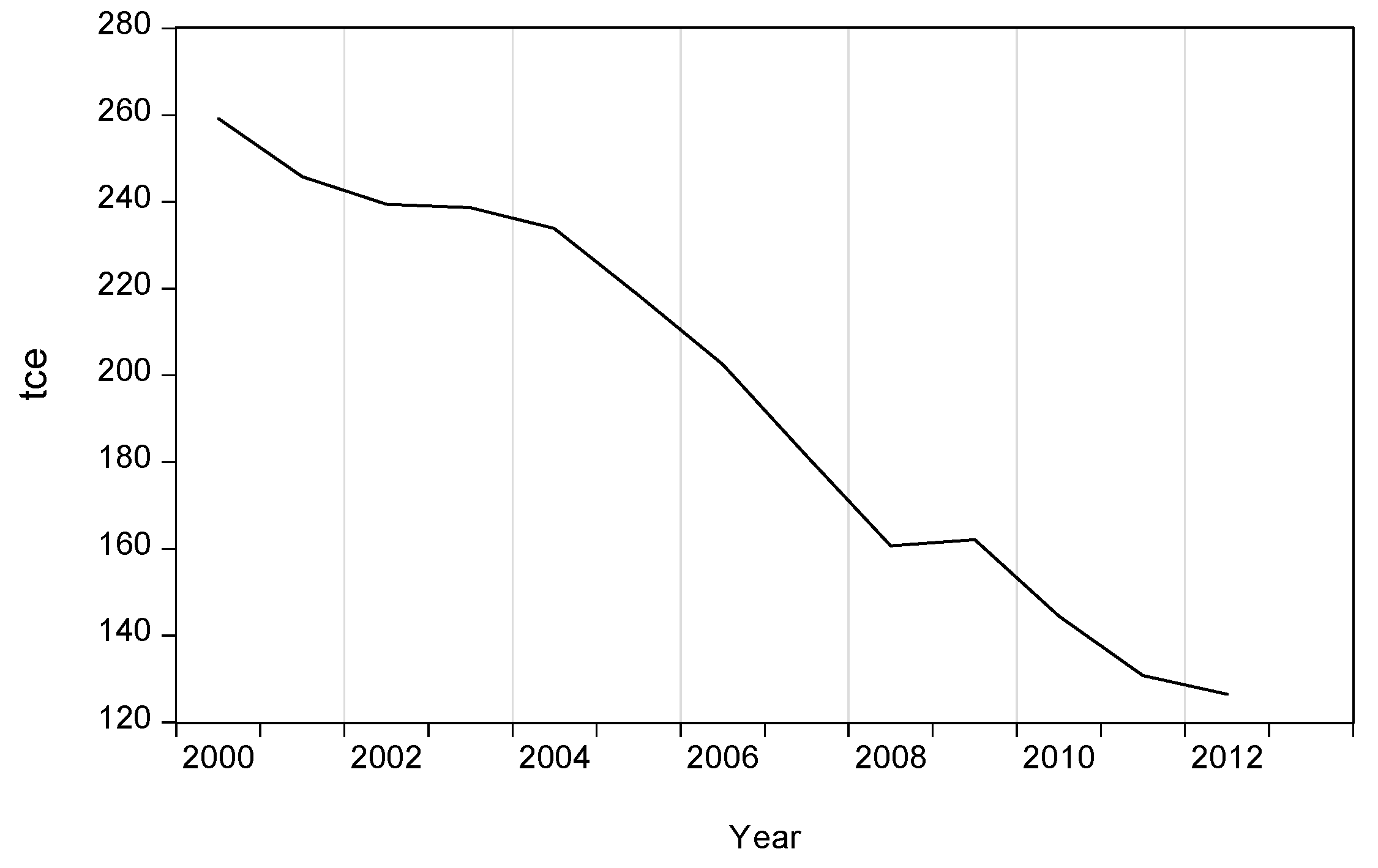
It is worth noting that although industrial output in 2013 was 2.73 times that of 2005, industrial energy consumption for a given output (one million RMB of industrial value added) has continued to drop since 2000 (Figure 2). The increase in industrial energy consumption had lagged behind that of China’s overall energy consumption (3617 million tce in 2012) (Figure 1). Thus, industrial energy efficiency appears to be improved. We argue that the use of energy-saving technologies may account for the negative effect of industrial output on energy prices.

7. Conclusions

Both occupations of real estate and industrial production consume a significant amount of energies in China. In theory, growing energy prices reduce the demand for real estate and depress industrial output. However, we found no long-term equilibrium relationship between these variables. It is possible that the lack of an empirical relationship is mainly due to the fact that energy prices in China have long been government-controlled. Such control measures tend to be counter cyclical, which reduces short-term price fluctuations. Energy price trends, in the long run, are still mainly shaped by market forces. The lack of long run equilibrium relationship is more likely to be a result of increasing use of energy-saving technologies in buildings, which is promoted government policies. As a result of government policy that encourages production of energy efficient buildings, less energy is consumed in new buildings, which can migrate the impact of an increase in energy prices on the operating cost of buildings and thus the demand for real estate will be less affected by energy prices in the long run.

We do not find any short-term dynamics between energy prices and the demand for housing. In addition to regulated energy prices, the lack of short-run relationship between energy prices and housing demand may also be due to the increase in housing vacancy rate in recent years as a result of an increase in speculative demand for housing. Since vacant housing units do not consume energy, an increase in the housing vacancy rate may disturb the short-term dynamics between housing sales and energy prices.

This, however, is not the case for the commercial real estate, which has a lower vacancy rate. We found commercial real estate sales lead energy prices but not vice versa. In theory, energy prices should lead demand for the commercial real estate if energy prices are market determined. However, government intervention may have delayed the response of energy prices to changes in market conditions. Therefore, commercial real estate sales may appear to lead energy price in the short run.

Lastly, we found a feedback but asymmetric, short-term relationship between energy prices and industrial production with a stronger energy prices impact on housing demand than vice versa. This suggests that energy is a significant input in the industrial production process. Rising energy prices will increase production cost and thus reduce industrial output. The much weaker reverse impact suggest that energy prices are exogenously determined.

We suggest that our findings are significant for macroeconomic forecasting. However, we examined the real estate market by simply removing some fundamentals such as supply, real estate prices and interest rate, which is a limitation of this research.

References

- NBSC. Statistical Data: Yearly Data. Available online: http://data.stats.gov.cn/easyquery.htm?cn=C01 (accessed on 7 July 2017).
- British Petroleum. Statistical Review of World Energy—Underpinning Data, 1965–2016. Available online: http://www.bp.com/en/global/corporate/energy-economics/statistical-review-of-world-energy/downloads.html (accessed on 5 March 2018).
- Wheaton, W.C. Real estate ‘cycles’: Some fundamentals. Real Estate Econ. 1999, 27, 209–230. [Google Scholar] [CrossRef]
- Zhang, W.; Yang, S. The influence of energy consumption of china on its real GDP from aggregated and disaggregated viewpoints. Energy Policy 2013, 57, 76–81. [Google Scholar] [CrossRef]
- Zou, G.; Chau, K.W. Short- and long-run effects between oil consumption and economic growth in China. Energy Policy 2006, 34, 3644–3655. [Google Scholar] [CrossRef]
- Hort, K. Prices and turnover in the market for owner-occupied homes. Reg. Sci. Urban Econ. 2000, 30, 99–119. [Google Scholar] [CrossRef]
- Berkovec, J.A.; Goodman, J.L. Turnover as a measure of demand for existing homes. Real Estate Econ. 1996, 24, 421–440. [Google Scholar] [CrossRef]
- Goodman, A.C.; Thibodeau, T.G. Housing market segmentation. J. Hous. Econ. 2004, 7, 121–143. [Google Scholar] [CrossRef]
- Ciuna, M.; Milazzo, L.; Salvo, F. A mass appraisal model based on market segment parameters. Buildings 2017, 7, 34. [Google Scholar] [CrossRef]
- Ruggiero, M.D.; Forestiero, G.; Manganelli, B.; Salvo, F. Buildings energy performance in a market comparison approach. Buildings 2017, 7, 14. [Google Scholar] [CrossRef]
- Deng, Y.; Li, Z.; Quigley, J.M. Economic returns to energy-efficient investments in the housing market: Evidence from singapore. Reg. Sci. Urban Econ. 2012, 42, 506–515. [Google Scholar] [CrossRef]
- Cerin, P.; Hassel, L.G.; Semenova, N. Energy performance and housing prices. Sustain. Dev. 2015, 22, 404–419. [Google Scholar] [CrossRef]
- Fuerst, F.; McAllister, P. Eco-labeling in commercial office markets: Do LEED and energy star offices obtain multiple premiums? Ecol. Econ. 2011, 70, 1220–1230. [Google Scholar] [CrossRef]
- Yoshida, J.; Sugiura, A. The effects of multiple green factors on condominium prices. J. Real Estate Financ. Econ. 2014, 50, 412–437. [Google Scholar] [CrossRef]
- Aroul, R.R.; Hansz, J. The value of “green”: Evidence from the first mandatory residential green building program. J. Real Estate Res. 2012, 34, 27–50. [Google Scholar]
- Jayantha, W.M.; Man, W.S. Effect of green labelling on residential property price: A case study in Hong Kong. J. Facil. Manag. 2013, 11, 31–51. [Google Scholar] [CrossRef]
- Ciochetti, B.A.; McGowan, M.D. Energy efficiency improvements: Do they pay? J. Sustain. Real Estate 2010, 2, 305–333. [Google Scholar]
- Hsueh, L.-M.; Gerner, J.L. Effect of thermal improvements in housing on residential energy demand. J. Consum. Aff. 1993, 27, 87–105. [Google Scholar] [CrossRef]
- Hamilton, I.G.; Steadman, P.J.; Bruhns, H.; Summerfield, A.J.; Lowe, R. Energy efficiency in the British housing stock: Energy demand and the homes energy efficiency database. Energy Policy 2013, 60, 462–480. [Google Scholar] [CrossRef]
- Quigley, J.M. The production of housing services and the derived demand for residential energy. RAND J. Econ. 1984, 15, 555–567. [Google Scholar] [CrossRef]
- Dinan, T.M.; Miranowski, J.A. Estimating the implicit price of energy efficiency improvements in the residential housing market: A hedonic approach. J. Urban Econ. 1989, 25, 52–67. [Google Scholar] [CrossRef]
- Zou, G.L.; Chau, K.W. Housing development, energy consumption and energy prices. Adv. Mater. Res. 2014, 853, 367–372. [Google Scholar] [CrossRef]
- Zou, G.L. Energy prices and housing property demand in Shanghai, China. Energy Sources Part B Econ. Plan. Policy 2013, 8, 1–6. [Google Scholar] [CrossRef]
- Humphreys, H.B.; McClain, K.T. Reducing the impacts of energy price volatility through dynamic portfolio selection. Energy J. 1998, 19, 107–131. [Google Scholar] [CrossRef]
- Mork, K.; Olsen, O.; Mysen, H. Macroeconomic responses to oil price increases and decreases in seven oecd countries. Energy J. 1994, 15, 19–36. [Google Scholar]
- Dudian, M.; Mosora, M.; Mosora, C.; Birova, S. Oil price and economic resilience. Romania’s case. Sustainability 2017, 9, 273. [Google Scholar] [CrossRef]
- Shi, X.; Sun, S. Energy price, regulatory price distortion and economic growth: A case study of China. Energy Econ. 2017, 63, 261–271. [Google Scholar] [CrossRef]
- Engle, R.F.; Granger, C.W.J. Cointegration and error correction: Representation, estimation and testing. Econometrica 1987, 55, 251–276. [Google Scholar] [CrossRef]
- Phillips, P.C.B.; Ouliaris, S. Asymptotic properties of residual based tests for cointegration. Econometrica 1990, 58, 165–193. [Google Scholar] [CrossRef]
- Johansen, S. Statistical analysis of cointegration vectors. J. Econ. Dyn. Control 1988, 12, 231–254. [Google Scholar] [CrossRef]
- Johansen, S. Estimation and hypotheses testing of co-integration vectors in gaussian vector autoregressive models. Econometrica 1991, 59, 1551–1580. [Google Scholar] [CrossRef]
- Haug, A.A. Critical values for the zα-Phillips-Ouliaris test for cointegration. Oxf. Bull. Econ. Stat. 1992, 54, 473–480. [Google Scholar] [CrossRef]
- Phillips, P.C.B. Optimal inference in cointegrated systems. Econometrica 1991, 59, 283–306. [Google Scholar] [CrossRef]
- Dickey, D.A.; Fuller, W.A. Distribution of the estimators for autoregressive time series with a unit root. J. Am. Stat. Assoc. 1979, 74, 427–431. [Google Scholar]
- Phillips, P.C.B.; Perron, P. Testing for a unit root in time series regression. Biometrika 1988, 75, 335–346. [Google Scholar] [CrossRef]
- Perron, P.; Ng, S. Useful modifications to some unit root tests with dependent errors and their local asymptotic properties. Rev. Econ. Stud. 1996, 63, 435–463. [Google Scholar] [CrossRef]
- Ng, S.; Perron, P. Lag length selection and the construction of unit root tests with good size and power. Econometrica 2001, 69, 1519–1554. [Google Scholar] [CrossRef]
- Elliott, G.; Rothenberg, T.J.; Stock, J.H. Efficient tests for an autoregressive unit root. Econometrica 1996, 64, 813–836. [Google Scholar] [CrossRef]
- Perron, P. The great crash, the oil price shock, and the unit root hypothesis. Econometrica 1989, 57, 1361–1401. [Google Scholar] [CrossRef]
- Perron, P. Further evidence on breaking trend functions in macroeconomic variables. J. Econom. 1997, 80, 355–385. [Google Scholar] [CrossRef] [Green Version]
- Sen, A. On unit-root tests when the alternative is a trend-break stationary process. J. Bus. Econ. Stat. 2003, 21, 174–184. [Google Scholar] [CrossRef]
- NBSC. Statistical Data: Monthly Statistics. Available online: http://data.stats.gov.cn/easyquery.htm?cn=A01 (accessed on 20 March 2018).
- NBSC. Statistical Data: Monthly data. Available online: http://data.stats.gov.cn/easyquery.htm?cn=A01 (accessed on 5 March 2016).
- Beijing Statistical Information Net. Statistical Terms. Available online: www.bjstats.gov.cn (accessed on 10 March 2017).
- CNPC. Oil Product Market: Domestic Gasoline and Diesel Wholesale Prices. Available online: http://www.cnpc.com.cn/cnpc/index.shtml (accessed on 5 May 2016).
- EIA. Data: Petroleum & Other Liquids Data. Available online: https://www.eia.gov/dnav/pet/hist/LeafHandler.ashx?n=pet&s=rwtc&f=m (accessed on 5 January 2018).
- CNgold Energy. Energy. Available online: http://energy.cngold.org/ (accessed on 9 January 2018).
- Cologni, A.; Manera, M. Oil prices, inflation and interest rates in a structural cointegrated var model for the g-7 countries. Energy Econ. 2008, 30, 856–888. [Google Scholar] [CrossRef]
- Kilian, L. The economic effects of energy price shocks. J. Econ. Lit. 2008, 871–909. [Google Scholar] [CrossRef]
- Abeysinghe, T. Deterministic seasonal models and spurious regressions. J. Econ. 1994, 61, 259–272. [Google Scholar] [CrossRef]
- Hendry, D.F.; Juselius, K. Explaining cointegration analysis: Part I. Energy J. 2000, 21, 1–42. [Google Scholar] [CrossRef]
- Newey, W.K.; West, K.D. A simple, positive semi-definite, heteroskedasticity and autocorrelation consistent covariance matrix. Econometrica 1987, 55, 703–708. [Google Scholar] [CrossRef]
- Ng, S.; Perron, P. Unit root tests in arma models with data dependent methods for the selection of the truncation lag. J. Am. Stat. Assoc. 1995, 90, 268–281. [Google Scholar] [CrossRef]
- MacKinnon, J.G. Numerical distribution functions for unit root and cointegration tests. J. Appl. Econ. 1996, 11, 601–618. [Google Scholar] [CrossRef]
- Hamilton, J.D. Time Series Analysis, 1st ed.; Princeton University Press: Princeton, NJ, USA, 1994. [Google Scholar]
- Banerjee, A.; Lumsdaine, R.L.; Stock, J.H. Recursive and sequential tests of the unit root and trend break hypothesis: Theory and international evidence. J. Bus. Econ. Stat. 1992, 10, 271–287. [Google Scholar]
- Hendry, D.F.; Juselius, K. Explaining cointegration analysis: Part II. Energy J. 2001, 22, 75–120. [Google Scholar] [CrossRef]
- Osterwald-Lenum, M. A note with quantiles of the asymptotic distribution of the maximum likelihood cointegration rank test statistics. Oxf. Bull. Econ. Stat. 1992, 54, 461–472. [Google Scholar] [CrossRef]
- MacKinnon, J.G.; Haug, A.A.; Michelis, L. Numerical distribution functions of likelihood ratio tests for cointegration. J. Appl. Econ. 1999, 14, 563–577. [Google Scholar] [CrossRef] [Green Version]
- Cheung, Y.-W.; Lai, K.S. Finite-sample sizes of johansen’s likelihood ratio tests for cointegration. Oxf. Bull. Econ. Stat. 1993, 55, 313–328. [Google Scholar] [CrossRef]
- Reinsel, G.C.; Ahn, S.K. Vector autoregressive models with unit roots and reduced rank structure: Estimation. Likelihood ratio test, and forecasting. J. Time Ser. Anal. 1992, 13, 353–375. [Google Scholar] [CrossRef]
- Wang, Q.; Qiu, H.-N.; Kuang, Y. Market-driven energy pricing necessary to ensure china’s power supply. Energy Policy 2009, 37, 2498–2504. [Google Scholar] [CrossRef]
- Paltsev, S.; Zhang, D. Natural gas pricing reform in china: Getting closer to a market system? Energy Policy 2015, 86, 43–56. [Google Scholar] [CrossRef]
- CNgold Energy. Historical Shanghai Gasoline Prices. Available online: https://www.cngold.org/crude/shanghai.html (accessed on 9 January 2018).
- Meng, B.; Zhang, J.; Qi, Z. A survey for Beijing ordinary residential vacancy. Urban Issue 2009, 4, 6–11. (In Chinese) [Google Scholar]
- Han, Y. An analysis of commodity residential vacancy. Henan Sci. Technol. 2011, 12, 22. (In Chinese) [Google Scholar]
- Chau, K.W.; Wong, S.K. Information asymmetry and the rent and vacancy rate dynamics in the office market. J. Real Estate Financ. Econ. 2016, 53, 1–22. [Google Scholar] [CrossRef]
- Zheng, J.J. Office market oversupply in large and medium-sized cities in China. China Bussiness Newspaper, 15 July 2014. (In Chinese) [Google Scholar]
Figure 1.
Energy consumption in China.
Figure 2.
Energy consumption per million RMB of industrial value added, China.