A Framework for the Selection of Optimum Offshore Wind Farm Locations for Deployment

Abstract

This research develops a framework to assist wind energy developers to select the optimum deployment site of a wind farm by considering the Round 3 available zones in the UK. The framework includes optimization techniques, decision-making methods and experts’ input in order to support investment decisions. Further, techno-economic evaluation, life cycle costing (LCC) and physical aspects for each location are considered along with experts’ opinions to provide deeper insight into the decision-making process. A process on the criteria selection is also presented and seven conflicting criteria are being considered for implementation in the technique for the order of preference by similarity to the ideal solution (TOPSIS) method in order to suggest the optimum location that was produced by the nondominated sorting genetic algorithm (NSGAII). For the given inputs, Seagreen Alpha, near the Isle of May, was found to be the most probable solution, followed by Moray Firth Eastern Development Area 1, near Wick, which demonstrates by example the effectiveness of the newly introduced framework that is also transferable and generic. The outcomes are expected to help stakeholders and decision makers to make better informed and cost-effective decisions under uncertainty when investing in offshore wind energy in the UK.

1. Introduction

The future of wind energy seems to keep growing as 18 GW are expected to be deployed by 2020 in the UK, with potential for more ambitious targets after 2020. Thus, there is a substantial need to reduce the cost of energy by identifying relevant cost reduction strategies in order to achieve these goals. The future of the UK’s industry size strongly depends on these goals [1]. Significant price increases in the overall cost of turbines, operations and maintenance have a direct impact on large-scale wind projects, hence the wind energy industry is determined to lower the costs of producing energy in all phases of the wind project from predevelopment to operations. Following the UK technology roadmap, the offshore wind costs should be reduced to £100/MWh by 2020 [2]. According to [1] the costs were stabilized at £140 per MWh in 2011. The UK’s Offshore Wind Programme Board (OWPB) stated that the offshore wind costs dropped below £100/MWh when 2015–2016 projects achieved a levelized cost of energy (LCOE) of £97 compared to £142 per MWh in 2010–2011, according to the Cost Reduction Monitoring Framework report in 2016 [3]. Recently, in 2017, Ørsted (formerly DONG Energy) guaranteed a £57.5/MWh building the world’s largest offshore wind farm in Hornsea 2, according to [4].

Developers and operators of offshore wind energy projects face many risks and complex decisions regarding service life cost reduction. In many cases, the manufacturers produce large volumes of parts in order to deal with the issue via economies of scale. Also, project consents can be time-consuming and difficult to obtain, however, all offshore wind farms were successfully completed regarding investment and profit [1]. Ensuring a long-term and profitable investment plan can be challenging, with both pre-consent and post-consent delays introducing considerable risks [2,5]. To this end, appropriate planning studies should be conducted at the early development stages of the project in order to minimize the investment risk. A breakdown of the key costs in an offshore wind farm can be found in [6] while studying existing projects, the location of a wind farm and the type of support structure have a great impact on the overall costs [7,8,9].

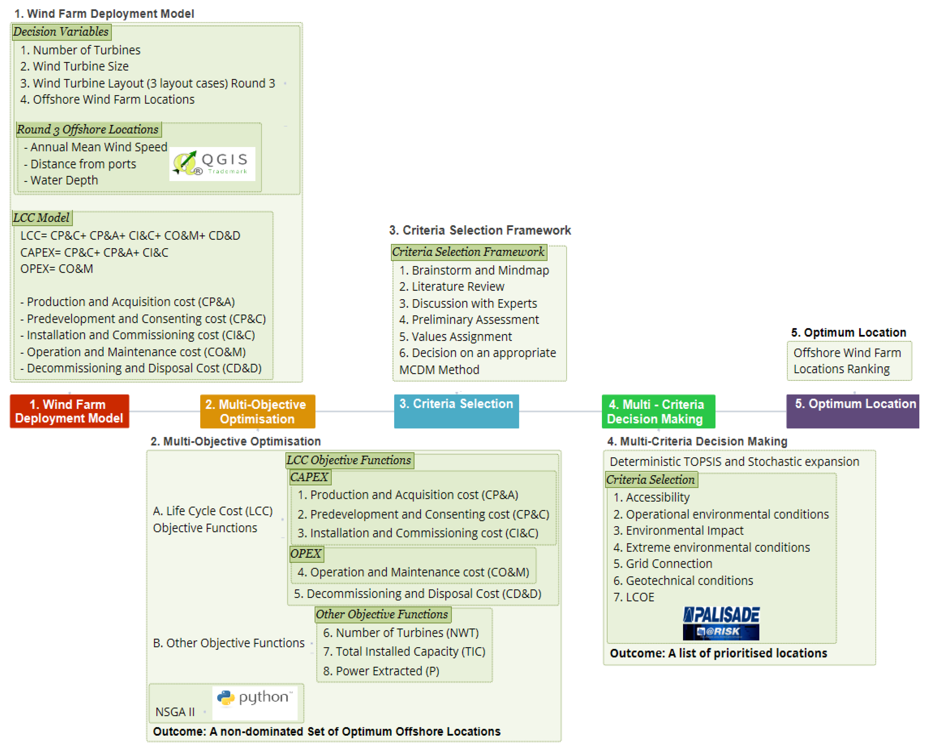
The aim of this paper is to develop a wind farm deployment framework, as illustrated in Figure 1, for supporting investment decisions at the initial stages of the development of Round 3 offshore wind farms in the UK by combining multi-objective optimization (MOO), life cycle cost (LCC) analysis and multicriteria decision making (MCDM). The contribution to knowledge is in developing and applying this novel and transferable framework that combines an economic analysis model by using LCC and geospatial analysis, MOO by using nondominated sorting genetic algorithm (NSGA II), survey data from real-world experts and finally MCDM by using a deterministic version and a stochastic expansion of the technique for the order of preference by similarity to the ideal solution (TOPSIS). Also, a criteria selection framework for the implementation of MCDM methods has been devised. The outcomes are expected to provide a deeper insight into the wind energy sector for future investments.

The structure of the remaining sections of this paper starts with a literature review on related studies for LCC analysis, turbine layout optimization, MCDM, and wind farm location selection in the offshore wind energy sector. Next, the development of the proposed framework is documented. The nondominated results for all zones will be analyzed and discussed followed by the prioritization process from TOPSIS. Conclusions and future work are documented at the end of the paper.

2. Literature Review

The Crown Estate has the rights of the seabed leasing up to 12 nautical miles from the UK shore and the right to exploit the seabed for renewable energy production up to 200 miles across its international waters. In recent years, the Crown Estate has run three rounds of wind farm development sites and their extensions. When the Crown Estate released the new Round 3 offshore wind site leases, they provided nine large zones of up to 32 GW power capacity [10]. The new leases encourage larger scale investments and consequently bigger wind turbines and include locations further away from the shore and in deeper waters [2,5,11,12,13].

Currently, all Round 3 zones have been suggested and published according to reports by the Department for Energy and Climate Change (DECC) and other stakeholders after the outcome of a strategic environmental assessment [14]. It should be noted that new offshore and onshore electricity transmission networks are needed in order to cover Round 3 connections up to 25 GW [14]. The Round 3 zones are the following; Moray Firth, Firth of Forth, Dogger Bank, Hornsea, East Anglia (Norfolk Bank), Rampion (Hastings), Navitus Bay (West Isle of Wight), Atlantic Array (Bristol Channel), and Irish Sea (Celtic Array). Every zone consists of various sites and extensions. Here, the five first zones in the North Sea are investigated in order to demonstrate the proof of the developed framework’s applicability. Each location faces similar challenges such as deep waters or long distances from the shore, etc. as shown in Figure 2.

Only a few location-selection-focused studies can be found, and usually, the findings and the formulation of the problems follow a different direction that this present study. For instance [15], uses goal programming in order to obtain the optimum offshore location for a wind farm installation. The study involves Round 3 locations in the UK and discusses its flexibility to combine decision-making. The work integrates the energy production, costs and multicriteria nature of the problem while considering environmental, social, technical and economic aspects.

For instance, the following literature presents cases in renewable energy where optimization has been successfully applied by utilizing different algorithms. An approach that links a multi-objective genetic algorithm to the design of a floating wind turbine was presented in [16]. By varying nine design variables related to the structural characteristics of the support structure, multiple concepts of support structures were modelled and linked to the optimizer. In [17], the authors provide a case study for the optimization of the electricity generation mix in the UK by using hybrid MCDM and linear programming and suggest a methodology to deal with the uncertainty that is introduced in the problem by the bias in experts’ opinions and other related factors. In [18], a structural optimization model for the support structures of offshore wind turbines was implemented by using a parametric Finite Element Analysis (FEA) analysis coupled with a genetic algorithm in order to minimize the mass of the structure considering multicriteria constraints.

LCC analysis evaluates costs, enabling suggestions in cost reductions throughout a project’s service life. The outcome of the analysis provides pertinent information in investments and can influence decisions from the initial stages of a new project [19]. In [20], a parametric whole life cost framework for an offshore wind farm and a cost breakdown structure was presented and analyzed, where the project is divided into five different stages; the predevelopment and consenting (C_P&C), production and acquisition (C_P&A), installation and commissioning (C_I&C), operation and maintenance (C_O&M), and decommissioning and disposal (C_D&D) stage. The advantages and disadvantages of the transition to offshore wind and an LCC model of an offshore wind development were proposed in [21]. However, the study mainly focused on a simplified model and especially the operation and maintenance stage of the LCC analysis, and it was suggested that there could be a further full-scale LCC framework in the future. In [22], a detailed failure mode identification throughout the service life of offshore wind turbines was performed and a review of the three most relevant end-of-life scenarios were presented in order to contribute to increase the return on investment and decrease the levelized cost of electricity. However, there are limited studies that integrate a high fidelity of life cycle cost (LCC) analysis into a multi-objective optimization (MOO) algorithm. LCC analysis gains more ground over the years because of the increased uncertainty of wind energy projects throughout their service life, including the cost of finance, the real cost of Operational Expenditure (OPEX) and the potential of service life extension.

MCDM is beneficial for policy-making through evaluation and prioritization of available technological options because of their ability to combine both technical and non-technical alternatives as well as quantitative and qualitative attributes in the decision-making process. A number of MCDM methods are applicable to energy-related projects, however, TOPSIS was selected because of the wide applicability of the method as can be found in literature and the connection of the method to numerous energy-related studies such as [23,24,25]. It is common to combine stochastic and fuzzy processes in order to deal with uncertain environments. In [23], Lozano-Minguez employed a methodology on the selection of the best support structure among three design options of an offshore wind turbine, considering a set of qualitative and quantitative criteria. A similar study was reported by Kolios in [26], extending TOPSIS to consider stochasticity of inputs.

Methods and techniques to cope with a high number of criteria and high dimensionality of decision-making problems are available in the literature. The multiple criteria hierarchy process (MCHP) [27,28,29] has been employed in order to deal with multiple criteria in decision-making processes. MCHP is usually employed in combination with outranking MCDM methods. Further applications can be found in [30,31].

In general, classifying criteria as either qualitative or quantitative is related to their nature and fidelity of the analysis. The employed decision-making methods can be based on priority, outranking, distance or combination of the three [32]. In [23], a decision-making study was conducted in three fixed wind turbine support structure types considering both quantitative and qualitative criteria while using TOPSIS. A decision-making study on floating support structures by combining both quantitative and qualitative criteria was presented in [33].

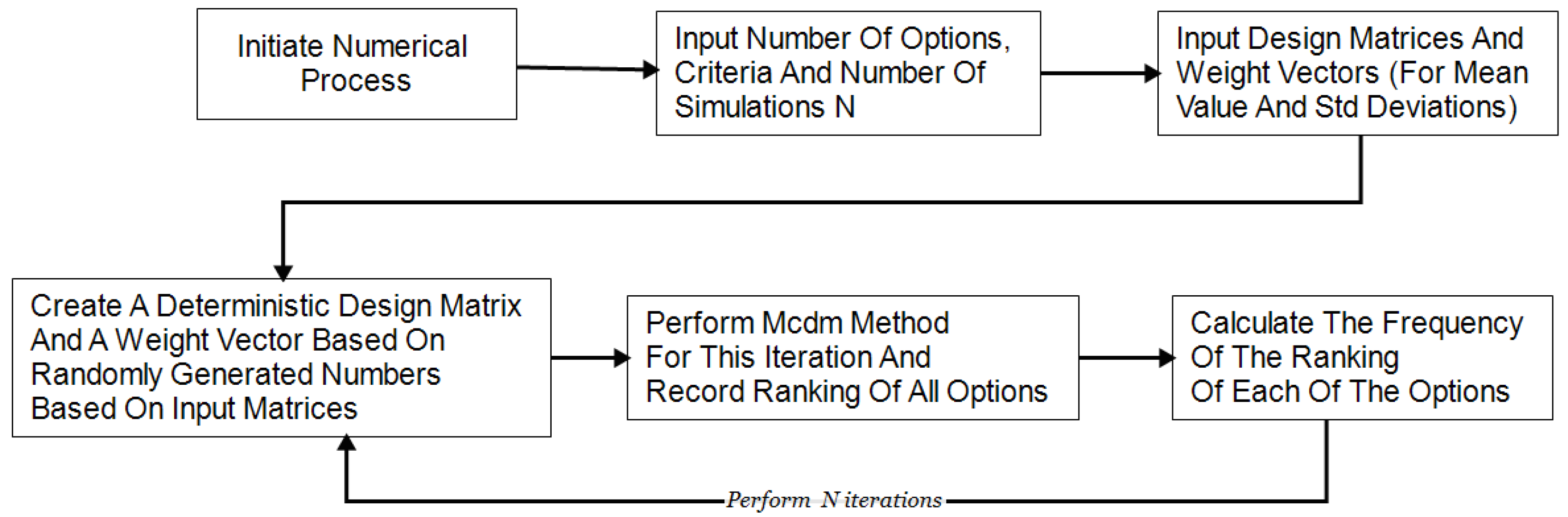
The approach proposed here for the stochastic expansion of deterministic methods was based in [26] that has reported the expansion of different deterministic methods, under the consideration that input variables are modelled as statistical distributions (derived by fitting data collected for each value in the decision matrix and weight vector), as shown in Figure 3. By using Monte Carlo simulations, numerous iterations quantify results and identify the number of cases where the optimum solution will prevail, i.e., there is a P_i probability that option X_i will rank first.

In [26], during deterministic TOPSIS, the weights for each criterion were considered fixed, but under stochastic modelling, statistical distributions were employed to best fit the acquired data of the experts’ opinions. Perera [34] has presented a study that combines MCDM and multi-objective optimization in the designing process of hybrid energy systems (HESs), using the fuzzy TOPSIS extension along with level diagrams. In [35], MCDM under uncertainty is discussed in an application where the alternatives’ weights are partially known. An extended and modified stochastic TOPSIS approach was implemented using interval estimations.

In [26], the authors extend the previous MCDM study on the decision-making of an offshore wind turbine support structure among different fixed and floating types. The decision matrix includes stochastic inputs (by using data from experts) in order to minimize the uncertainties in the study. In the same study, an iterative process has been included, and the TOPSIS method was implemented. In [36], a study suggests a methodology for classification and evaluation of 11 available offshore wind turbine support structure types while considering 13 criteria by using TOPSIS as the decision-making method.

In [24], an expansion of MCDM methods to account for stochastic input variables was conducted, where a comparative study was carried out by utilizing widely applied MCDM methods. The method was applied to a reference problem in order to select the best wind turbine support structure type for a given deployment location. Data from industry experts and six MCDM methods were considered, so as to determine the best alternative among available options, assessed against selected criteria in order to provide a level of confidence to each option.

An electricity generation systems allocation optimization model is suggested in [37] for the case of a disaster relief camp in order to minimize the total project cost and maximize the share of systems that were assessed through a decision-making process and were prioritized accordingly. Bi-objective integer linear programming and a decision-making method (VIKOR) were employed and the overall model was applied to a hypothetical map.

A study performed in [38] uses a TOPSIS model by incorporating technical, environmental and social criteria and finally combines the evaluation scores to develop a MOGLP (multi-objective grey linear programming) problem in order to assess the decision-making of power production technologies. The outcome of this work was the optimal mix of electricity generated by each option in the UK energy market. In [39], a methodology for an investment risk evaluation and optimization is suggested in order to mitigate the risks and achieve sustainability for wind energy projects in China. In this study, Monte Carlo analysis and a multi-objective programming model are used so as to increase the confidence in the planning of investment research and the sustainability of renewables in China.

In this study, NSGA II is employed because it is suitable for MOO problems with many objectives and was further analyzed in previous studies in offshore wind energy applications in [40], where a methodology was proposed to support the decision-making process at these first stages of a wind farm investment considering available Round 3 zones in the UK. Three state-of-the-art algorithms were applied and compared to a real-world case of the wind energy sector. Optimum locations were suggested for a wind farm by considering only round 3 zones around the UK. The problem comprised of techno-economic Life Cycle Cost related factors, which were modelled by using the physical aspects of each wind farm location (i.e., the wind speed, distance from the ports and water depth), the wind turbine size and the number of turbines.

3. Framework

3.1. Wind Farm Deployment Model

The wind farm deployment model implemented in this study couples the LCC analysis with a geospatial analysis as described below. The LCC analysis of a project involves all project stages described in Figure 4. In [20,41], a whole LCC formulation is provided, and this study integrates these phases into the MOO problem. Assumptions and related data in the modelling of the problem were gathered from the following references [20,41,42,43,44,45,46] based on which the present model was developed. The LCC model described in [20] is used as a guideline in this study, and along with the site characteristics and the problem’s formulation, the optimization problem is formed. The type of foundation that was considered in the LCC model is the jacket structure as it constitutes a configuration that can be utilized in a range of water depths allowing for the optimization process to be automated.

The total LCC is calculated as follows:

LCC = C_P&C + C_P&A + C_I&C + C_O&M + C_D&D

(1)

where

• LCC: Life Cycle Cost
• C_I&C: Installation and Commissioning cost
• C_P&C: Predevelopment and Consenting cost
• C_O&M: Operation and Maintenance cost
• C_P&A: Production and Acquisition cost
• C_D&D: Decommissioning and Disposal Cost

CAPEX = C_P&C + C_P&A + C_I&C

(2)

OPEX = C_O&M

(3)

• CAPEX: Capital expenditure
• OPEX: Operational expenditure

The power extracted is calculated for each site and each wind turbine respectively as:

$$P=\frac{1}{2}ACp\rho u^3$$

(4)

where

• $A:$ Turbine rotor area
• $\rho$: Air density
• C_p: Power coefficient
• $u:$ Mean annual wind speed of each specific site

The total installed capacity (TIC) of the wind farm dependents on the number of turbines and the rated power of each of them, and is calculated for every solution:

$$\mathrm{TIC}={\mathrm{P}}_{\mathrm{R}}\times \mathrm{NWT}$$

(5)

where

• ${\mathrm{P}}_{\mathrm{R}}$: Rated power
• NWT: Number of turbines

For each offshore location, a special profile was created including the coordinates, distance from designated construction ports, annual wind speed and average site water depth, as listed in

Table 1. Round 3 zones and sites, and specific data acquired from [45].

Site Index	Zone	Wind Farm Site Name	Centre Latitude	Centre Longitude	Port	Distance from the Port (km)	Annual Wind Speed (m/s) (at 100 m)	Average Water Depth (m)
0	Moray Firth	Moray Firth Western Development Area	58.097	−3.007	Port of Cromarty	123.691	8.82	44
1	Moray Firth	Moray Firth Eastern Development Area 1	58.188	−2.720	Port of Cromarty	157.134	9.43	44.5
2	Firth of Forth	Seagreen Alpha	56.611	−1.821	Montrose	72.598	9.92	50
3	Firth of Forth	Seagreen Bravo	56.572	−1.658	Montrose	91.193	10.09	50
4	Dogger Bank	Creyke Beck A	54.769	1.908	Hartlepool and Tess	343.275	10.01	21.5
5	Dogger Bank	Creyke Beck B	54.977	1.679	Hartlepool and Tess	319.949	10.04	26.5
6	Dogger Bank	Teesside A	55.039	2.822	Hartlepool and Tess	447.124	10.05	25.5
7	Dogger Bank	Teesside B	54.989	2.228	Hartlepool and Tess	380.788	10.04	25.5
8	Hornsea	Hornsea Project One	53.883	1.921	Grimsby	242.328	9.69	30.5
9	Hornsea	Hornsea Project Two	53.940	1.687	Grimsby	217.270	9.73	31.5
10	Hornsea	Hornsea Project Three	53.873	2.537	Grimsby	310.521	9.74	49.5
11	Hornsea	Hornsea Project Four	54.038	1.271	Grimsby	173.928	9.71	44.5
12	East Anglia (Norfolk Bank)	East Anglia One	52.234	2.478	Great Yarmouth	92.729	9.5	35.5
13	East Anglia (Norfolk Bank)	East Anglia One North	52.374	2.421	Great Yarmouth	81.104	9.73	45.5
14	East Anglia (Norfolk Bank)	East Anglia Two	52.128	2.209	Great Yarmouth	74.559	9.46	50
15	East Anglia (Norfolk Bank)	East Anglia Three	52.664	2.846	Great Yarmouth	124.969	9.56	36
16	East Anglia (Norfolk Bank)	Norfolk Boreas	53.040	2.934	Great Yarmouth	143.464	9.53	31.5
17	East Anglia (Norfolk Bank)	Norfolk Vanguard	52.868	2.688	Great Yarmouth	111.449	9.56	32

, where data was acquired from [45]. Among various data, Table 1 shows the locations that each of these zones contains.

For the distances from the ports calculation an open source licensed geographic information system (GIS) called QGIS was used, which is a part of the Open Source Geospatial Foundation (OSGeo) [47]. A list of ports was acquired from [48,49,50]. The QGIS maps of the offshore sites were acquired from the official Crown Estate website [51] for QGIS and AutoCAD. The list contains designated, appropriate and sufficient construction ports that are suitable for the installation, manufacturing and maintenance for wind farms. New ports are to be built specifically to accommodate needs of the offshore wind industry; however, this study takes into account a selection of currently available ports around the UK. The distances were calculated assuming that the nearest port to the individual wind farm is connected in a straight line. QGIS was also employed to measure and model aspects of the LCC related to the geography and operations. The estimated metrics were integrated into the configuration settings of the whole LCC.

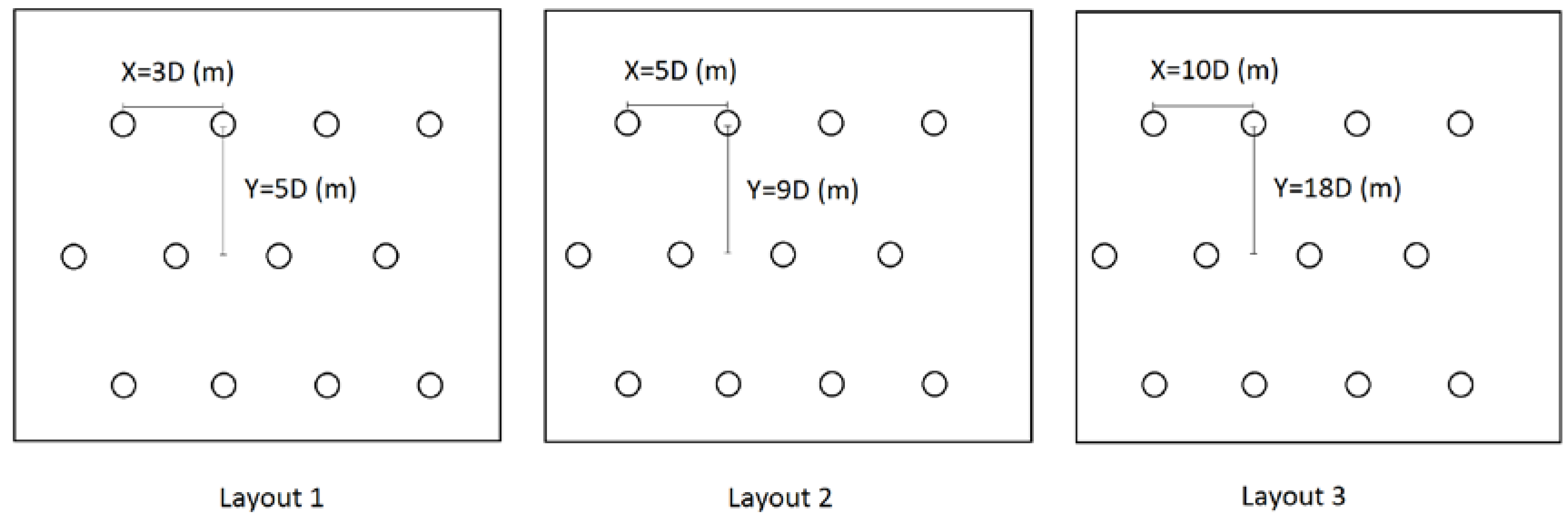
Three layout configurations are considered. The lower and upper limits of a theoretical array layout from [52] will be employed along with an extreme case. More specifically, in the lower limit case (layout 1), the horizontal and vertical distance between turbines is 3 and 5 times the rotor diameter, respectively. The turbine specifications used for the LCC model are listed in

Table 2. Turbine specifications.

Turbine Type Index	Rated Power (MW)	Rotor Diameter (m)	Hub Height (m)	Total Weight (t)
0	10	190	125	1580
1	8	164	123	965
2	7	154	120	955
3	6	140	100	656

. In the upper limit case (layout 2), 5 and 9 times the rotor diameter were considered horizontally and vertically. In the extreme case (layout 3), the horizontal and vertical distance between turbines is 10 and 18 times the rotor diameter. All different configurations are illustrated in Figure 5. The present work focuses on the optimization of offshore wind farm locations considering the maximum wind turbine number that can fit in the selected Round 3 locations according to three different layout configuration placements. The wind farm is oriented according to the most optimal wind direction. Different layouts provide a different maximum wind turbine number that can guide the optimization process to more detailed calculations. The maximum number of wind turbines is determined by considering types of reference turbines of 6, 7, 8 and 10 MW and by following three layout cases, as listed below in Figure 5, where D is the diameter of each turbine.

For the estimation of cabling length, which is required to calculate parts of the LCC related to the spatial distribution of the wind turbines in the wind farm, the minimum spanning tree algorithm is used. The location of the turbines is treated as a vertex of a graph, and the cabling represents the edge that connects the vertices. Given a set of vertices, which are separated by each other by the different layout indices, from Figure 5, the minimum spanning tree connects all these vertices without creating any cycles, thus yielding minimum possible total edge length. This represents the minimum cabling length of the particular layout.

The way the length of the cables was calculated provides an approximation of the actual length. In the presence of relevant actual data, the calculations of both the layouts and the LCC would provide more realistic values. For instance, the cable length would be expected to be larger because of the water depth and the burial of the cables for each turbine. For each cable, both ends will have to come from the seabed to the platform, so at least twice the water depth should be added to each cable and finally allow for some contingency length for installation.

The wind rose diagrams provided the prevailing wind direction, which sets the layout orientation. The wind speeds, the wind rose graphs, and the coordinates of each location were obtained by FUGRO (Leidschendam, The Netherlands) and 4COffshore (Lowestoft Suffolk, UK) [45,53]. All wind farm sites were discovered to have dominant southwestern winds followed by western winds. For that reason, the orientation of the layouts is assumed to be southwestern (as the winds are assumed to blow predominantly from that direction). The wind rose graphs for each offshore site are determined by data acquired from [53] and the grid points they created around the UK. The nearest grid point to the offshore site is used.

An important factor to be considered is also the atmospheric stability. Although the different layouts considered in this study may be affected by the atmospheric stability states, as it impacts the layout’s wake recovery pattern, it was not considered in the framework. Also, the power curves and their multiplicity in turbine type were not considered in this study because the aim is to devise and demonstrate a generic and transferable methodology. It is suggested that both elements could be further investigated in future studies to evaluate their effect in the derivation of the optimum solution.

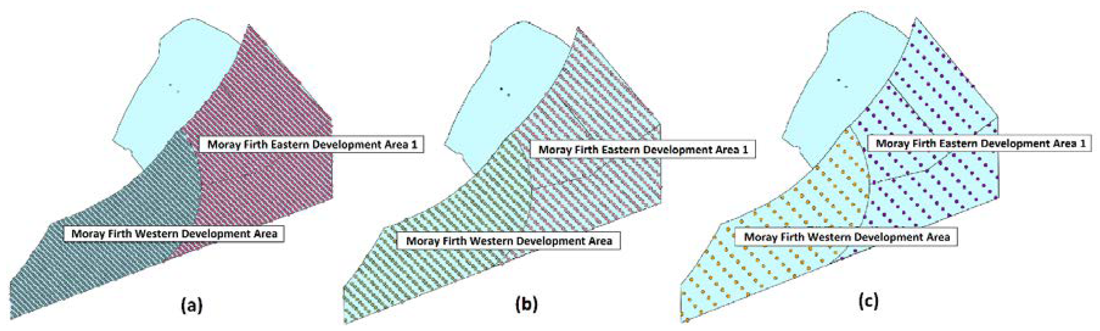
In Figure 6, the example of Moray Firth zone (which includes Moray Firth Western Development Area and Moray Firth Eastern Development Area 1) shows the positioning of the turbines depending on the layout 1, 2 and 3 and the turbine size.

3.2. Multi-Objective Optimization

The optimization problem includes eight objectives; five LCC-related objectives, based on [20], which are the cost-related objectives to be minimized. The three additional objectives are the number of turbines (NWT), the power that is extracted (P) from each offshore site and the total installed capacity (TIC), which are to be minimized, maximized, and maximized, respectively.

More specifically, the LCC includes the predevelopment and consenting, production and acquisition, installation and commissioning, operation and maintenance and finally decommissioning and disposal costs. The power extracted is calculated by the specific mean annual wind speed of each location along with the characteristics of each wind turbine both of which are considered inputs.

The optimization problem formulates as follows:

Minimize  C_P&C, C_P&A, C_I&C, C_O&M, C_D&D, NWT, (−P), (−TIC)

(6)

Subject to $0\le \text{site index}\le 20$,

     $0\le \text{turbine type index}\le 3$

     $1\le \text{layout index}\le 3$

     $50\le \text{Number of turbines}\le \text{maximum number per site}$

     $\mathrm{TIC}\le \text{Maximum capacity of Round 3 sites based on the Crown Estate}$

Although the maximum number of turbines has been estimated by using QGIS, the maximum capacity allowed per region was also considered, as specified by the Crown Estate, as listed in

Table 3. Maximum capacity of Round 3 wind farms, specified by the Crown Estate [1].

Zone	Capacity (MW)
1. Moray Firth	1500
2. Firth of Forth	3465
3. Dogger Bank	9000
4. Hornsea	4000
5. East Anglia	7200
6. Rampion	665
7. Navitus Bay	1200
8. Bristol Channel	1500
9. Celtic Array	4185
TOTAL CAPACITY	32,715

. These were selected because of the possibility that the constraints might overlap in an extreme case scenario. Therefore, both constraints were added to the problem in order to secure all cases.

The optimization part of the framework has been implemented in Python 3, employing library ‘platypus’ in Python [54].

3.3. Criteria Selection Process

For the MCDA, the criteria selection process follows the process illustrated in Figure 7:

• The first step is to create a mind map of the problem and the different aspects involved. Then, via brainstorming, criteria that can potentially impact on the alternatives of the problem are listed.
• The second step is to perform an extensive literature review on the topic. It is vital that the literature review is conducted in order to discover related studies and also confirm or reject ideas that were found in the first step. During this process, it is possible to discover gaps that will help to define the study more precisely and also discover criteria that were never considered before.
• Step three is about discussing ideas with subject matter experts and communicating to them the aims and ideas of the project in order to obtain useful insights into the initial stages of the criteria selection. Their expertise can confirm, discard or suggest new criteria according to their opinion. Experts can also provide helpful data and confirm the value of the study.
• In step four, the strengths and weaknesses of the work and criteria should be identified, followed by a preliminary assessment. The selected criteria should be clear and precise, and no overlaps should be present (avoiding similar terms or definitions that can potentially include other criteria). Each criterion should characterize and affect the alternatives in a different and unique way. None of the criteria should conflict with each other. The criteria should now have a detailed description. Their description and explanation should be unique to avoid confusion especially if the criteria are sent to experts in the form of a survey.
• Step five describes how to proceed with the study. Assigning values to the criteria can be done either by calculating the values directly or by extracting them from the experts via a questionnaire. In the latter case, additional data or opinions could be considered. Via a survey, experts could either assign values or rate the criteria according to their knowledge and experience. Here, it is important to note that for a different set of criteria, different approaches can be followed. For example, in the case of criteria that need numerical values (and probably require calculations) that no expert can provide on the spot, receiving replies is challenging. The experts should provide their expertise in an easy and fast process. The definition of the criteria has to be very clear before scoring, normally at a scale of 1 to 5 or otherwise. The calculations could lead to assigned values for every criterion, but the experts could provide further insight regarding the importance of those criteria and how much they affect the alternatives. In this case, the experts provide the weights of the criteria, which is very useful in order to achieve higher credibility of the problem. In some cases, it would be very useful to include validation questions in the survey. It would also be useful to include questions in order to increase the validity of the problem, for example, to ask for further criteria that were not considered in the study. Another example would be to include a question about the perceived expertise of the experts that will answer the questionnaire. Hence, their answers will be weighted and further credible.
• Step six is related to selecting a method for decision-making. In general, it is important to decide quite early which method of the multicriteria analysis will be used. This is important because different methods require different criteria and problem set up. In the case of hierarchy problems and pairwise comparisons, the problem has to be set up differently, and the values need to be set for every pair comparison. The important question here is how the outcomes are derived. Having a picture of the total process and aims, objectives and results early enough can help to speed up the process.

3.4. Multicriteria Decision Making

Following the process of MOO and criteria selection, two versions of the MCDM method were implemented (i.e., deterministic and stochastic TOPSIS) and were linked to the results of the previous outcomes, as shown in Figure 1. A set of qualitative and quantitative criteria is combined in order to investigate the diversity and outcomes obtained from different sets of inputs in the decision-making process. Stochastic inputs are selected and imported in TOPSIS. All data were collected from industry experts, so as to prioritize the alternatives and assess them against seven selected conflicting criteria. The outcome of the method is expected to assist stakeholders and decision makers to support decisions and deal with uncertainty, where many criteria are involved.

TOPSIS is depicted in Figure 8, initially proposed by Hwang et al. [55], and the idea behind it lies in the optimal alternative being as close in the distance as possible from an ideal solution and at the same time as far away as possible from a corresponding negative ideal solution. Both solutions are hypothetical and are derived from the method. The concept of closeness was later established and led to the actual growth of the TOPSIS theory [56,57].

After defining $n$ criteria and $m$ alternatives, the normalized decision matrix is established. The normalized value $r_{ij}$ is calculated from the equations below, where $f_{ij}$ is the $i$-th criterion value for alternative $A_j$ ($j=1,\dots ,m$ and $i=1,\dots ,n$).

$$r_{ij}=\frac{f_{ij}}{\sqrt{{\sum }_{j=1}^m{f}_{ij}^2}}$$

(7)

The normalized weighted values $v_{ij}$ in the decision matrix are calculated as follows:

$$v_{ij}=w_i{r}_{ij}$$

(8)

The positive ideal $A^{+}$ and negative ideal solution $A^{-}$ are derived as shown below, where $I^{\prime }$ and $I^{″}$ are related to the benefit and cost criteria (positive and negative variables).

$$A^{+}=\left\{v_1^{+},\dots ,v_n^{+}\right\}=\left\{\left(MA{X}_j{v}_{ij}|i\in I^{\prime }\right),\left(MI{N}_j{v}_{ij}|i\in I^{″}\right)\right\}$$

(9)

$$A^{-}=\left\{v_1^{-},\dots ,v_n^{-}\right\}=\left\{\left(MI{N}_j{v}_{ij}|i\in I^{\prime }\right),\left(MA{X}_j{v}_{ij}|i\in I^{″}\right)\right\}$$

(10)

From the $n$-dimensional Euclidean distance, $D_j^{+}$ is calculated below as the separation of every alternative from the ideal solution. The separation from the negative ideal solution follows:

$$D_j^{+}=\sqrt{{\displaystyle \sum _{i=1}^n}{\left(v_{ij}-v_i^{+}\right)}^2}$$

(11)

$$D_j^{-}=\sqrt{{\displaystyle \sum _{i=1}^n}{\left(v_{ij}-v_i^{-}\right)}^2}$$

(12)

The relative closeness to the ideal solution of each alternative is calculated from:

$$C_j=\frac{D_j^{-}}{\left(D_j^{+}+D_j^{-}\right)}$$

(13)

After sorting the $C_j$ values, the maximum value corresponds to the best solution to the problem.

A survey that considers all seven criteria was created and disseminated to industry experts, so as to obtain the weights for the following MCDM study. In this case, experts provided their opinions based on the importance of each criterion in the wind farm location selection process. In total, 13 experts (i.e., academics, industrial experts and university partners) with relative expertise responded and rated the criteria according to their importance. The total number of 13 experts is considered sufficient for this work because the overall number of offshore wind experts is very limited and their engagement is challenging. The input data from the 13 experts were acquired through an online survey platform where the perceived level of expertise was also provided. The assessments varied between 2 and 5 (with 1 being a non-expert and 5 being an expert) with a mean value of 3.8 and a standard deviation of 0.89.

The implementation of the stochastic version of TOPSIS was modelled through Palisade’s software @Risk 7.5. Specifically, for the stochastic implementation, the Monte Carlo simulations of @Risk were combined with the survey data, providing the best distribution fit for each value to be used as inputs in the decision matrix of TOPSIS. By separately conducting a sensitivity analysis among 100, 1000, 10,000 and 100,000 iterations, 10,000 iterations for a simulation were found to deliver satisfactory results on acceptable computational effort requirements. Next, the stochastic approach is compared to the deterministic one and finally, the outcomes are presented in the next section.

All criteria and the final decision-making matrices were scaled and normalized, respectively in different phases of the process, while the seven criteria used in this study include both qualitative and quantitative inputs. Combining these two types can help decision makers to define their problems in a more reliable method. Next, both deterministic and stochastic approaches will be conducted and compared. The criteria are listed in

Table 4. List of criteria.

Criteria	ID
1. Accessibility	C1
2. Operational environmental conditions	C2
3. Environmental Impact	C3
4. Extreme environmental conditions	C4
5. Grid Connection	C5
6. Geotechnical conditions	C6
7. LCOE	C7

.

The criteria were selected based on literature and a brainstorming session with academic and industrial experts. In the session, common criteria were consolidated in order to avoid double counting and finally concluded to the ones used in the study. The criteria were selected such as to have both a manageable number and to cover all aspects but at the same time not make the data collection questionnaire too onerous.

More specifically, the criteria are defined and analyzed below:

• Accessibility: This criterion considers the accessibility of each wind farm by considering the distance from the ports and the number of nearby wind farms. The distances were acquired from the 4COffshore database [58]. The number of nearby wind farms was acquired from the interactive map of 4COffshore [45]. In order to select the number of nearby farms, only the farms that already produce energy and are located between the ports and the wind farm in question were considered. The nearby wind farms and the distance from the ports were assessed from 1 to 9 (1 being not close to any wind farms and 9 being close to many wind farms) and 9 to 1 (9 being very close to the ports and 1 being extremely far from the shore) respectively for each offshore site. The weighted values (equally weighted by 50–50) then were summed. This criterion is qualitative, and it varies from 1 to 9 (1 being not at all accessible to 9 extremely accessible). This criterion is also considered positive in the MCDM process. Both in the deterministic and stochastic processes, the values used are the same.
• Operational environmental conditions: This criterion considers the aerodynamic loads in the deployment location. More specifically, the wind speed (m/s) in specific points (close to each offshore sites) according to [53]. The criterion is quantitative and also positive. In the stochastic and deterministic approach, the fitted wind distributions and the mean values were used, respectively.
• Environmental impact: This criterion considers the structures’ greenhouse gas emissions during the construction and installation phase. The amount of CO₂ equivalent (CO₂e) emissions per kg of steel was estimated relative to the water depth (maximum and minimum water depth were measured in each location) and the distance from the ports. The support structure was assumed to be the jacket structure. This criterion was calculated according to an empirical formula in [23], and the water depth and distance from the ports were both considered in these calculations. Finally, an index of the square of CO₂ equivalent (CO₂e²) was considered from the two cases as a value for each offshore site. This criterion is negative. The criterion is also quantitative, and for the stochastic approach, a triangle distribution was considered. In the deterministic approach, the mean value was used.
• Extreme environmental conditions: This criterion considers the durability of the structure due to extreme aerodynamic environmental loads. Data were extracted from [53]. The wind distributions that represent the probabilities above the cut off wind speed (i.e., approximately 25 m/s) were considered. This criterion is quantitative and negative. For the stochastic approach, a triangle distribution was considered. In the deterministic approach, the mean values were used.
• Grid connection: This criterion considers the possible grid connection options of a new offshore wind farm (connection costs to existing or new grid points). The inputs of this criterion consider the cost (£million) of connecting to nearby substations where other Rounds already operate, extending existing ones or building new ones. In the national grid report that was created for the Crown Estate in [14], the costs were calculated by considering more than one cases per Round 3 location. In this study, the maximum and the minimum costs were considered, and a uniform distribution was used as a stochastic input. In the deterministic approach, the mean value is used. The criterion is quantitative and represented by the above cost values, and it is considered negative.
• Geotechnical conditions: This criterion represents the compatibility of the soil of each of the offshore locations for a jacket structure installation. Experts provided their input and rated the offshore locations according to their soil suitability from 1 to 9 (1 being very unsuitable to 9 being extremely suitable). This criterion is qualitative and positive. For the stochastic approach, a pert distribution was considered. In the deterministic approach, the mean value was used.
• Levelized cost of electricity (LCoE): This criterion considers an estimation of the LCoE for each offshore location (2015 £/MWh). The values were calculated according to the DECC simple levelized cost of energy model in [59]. The calculations assumed an 8 MW size turbine. Jacket structure and a range of water depths (maximum and minimum water depth measured in each site) per offshore site. The criterion is quantitative and negative. In the stochastic approach, the triangle distribution was used and in the deterministic, the mean value.

This study considered the criteria that have greater impact than others in the final decision-making process by assigning weights derived from the insights of experts.

It should be noted that some aspects were excluded for this analysis as they do not appear to affect the location selection process or they already included in the existing selected criteria and other steps of the framework. Fisheries and aquaculture is a criterion that considers the positive effects of the aquaculture and the fisheries around the wind farms. The criterion could be assessed according to similar fisheries and aquacultures that seem to benefit from nearby wind farms. This information is hard to obtain systematically or does not meet the unique characteristics of the wind farm locations. Regarding the environmental extensions, such as birds and fish, these were not considered in the environmental impact criterion. The Department for Energy and Climate Change conducted a strategic environmental assessment on the offshore sites for over 60m of water depth around the UK and the Crown Estate identified possible suitable areas for offshore wind farm deployments aligned with government policy and released the 3 Rounds [11,13]. Further, service life extension will not be considered because of the nature of the problem. In order to consider life extension, a sample of individual turbines is monitored, tested and investigated. There is no evidence whether there is a link of life extension possibility to the offshore location. Finally, marine growth or artificial reefs will not be included in the study because it does not reveal the uniqueness of the offshore sites. Marine growth exists in all offshore structures.

4. Results and Discussion

The data obtained from the experts were analysed and used in MCDM both deterministically and stochastically. The results from all locations (from all five zones) are provided and illustrated in Figure 9 as cost breakdown analysis. All 7 solutions shown and discussed were obtained from the execution of the NSGA II, and they are equally optimal solutions, according to the Pareto equality. 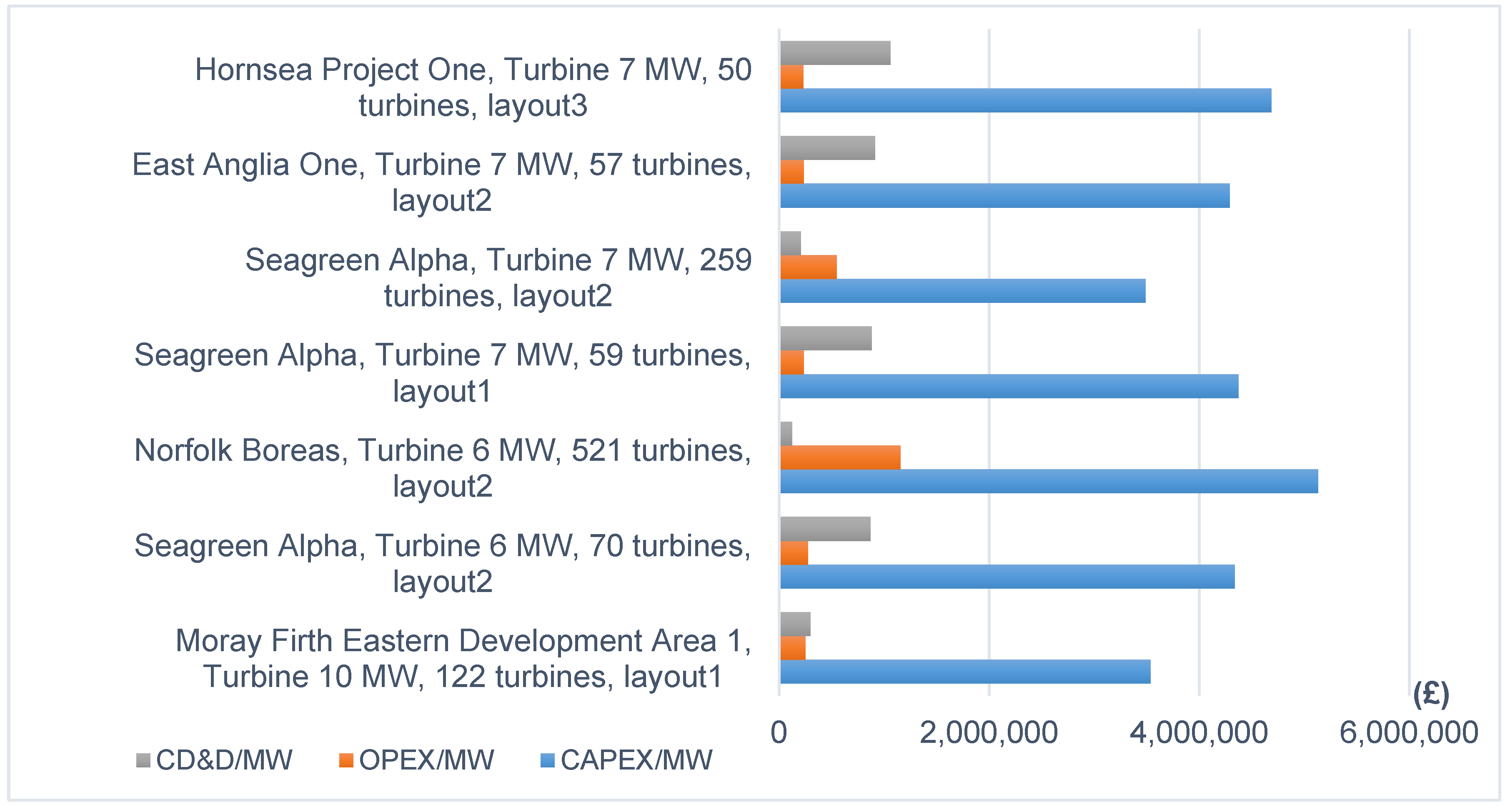The problem considered all 18 sites from the five selected Round 3 zones and the optimum results minimize CAPEX, OPEX and C_D&D, as shown in Figure 9. At the same time, the remaining objectives are also optimized. All layouts were found to deliver optimal solutions, where layout 3 was found only once with few turbines.

All optimal solutions are listed in

Table 5. Numerical results for all zones.

Offshore Wind Farm Site	Layout Selected	Turbine Size (MW)	NWT	OPEX (£)	CD&D [£]	CAPEX [£]	Total Cost [£]
Moray Firth Eastern Development Area 1	layout 1	10	122	307,322,672	365,371,991	4,316,454,016	4,989,148,680
Seagreen Alpha	layout 2	6	70	115,563,086	365,329,300	1,821,862,415	2,302,754,802
Norfolk Boreas	layout 2	6	521	3,612,087,515	383,807,107	16,034,493,829	20,030,388,452
Seagreen Alpha	layout 1	7	59	97,590,070	363,801,519	1,806,818,815	2,268,210,405
Seagreen Alpha	layout 2	7	259	996,944,713	373,550,029	6,323,114,490	7,693,609,234
East Anglia One	layout 2	7	57	93,654,614	364,474,208	1,712,388,330	2,170,517,154
Hornsea Project One	layout 3	7	50	81,096,384	371,523,572	1,640,942,787	2,093,562,744

. The solution that includes Hornsea Project One and layout 3 delivered the lowest costs of the optimal solutions. Although that was expected as it was found that only 50 turbines were selected by the optimizer, the same solution is the second most expensive per MW as shown in Figure 9. Moray Firth Eastern Development Area 1 could deliver the lowest cost per MW. The three solutions of the Seagreen Alpha included both layouts 1 and 2. The fact that Seagreen Alpha was selected three times shows the flexibility of multiple options for a suitable budget assignment that the framework can deliver to the developers. The C_D&D presents low fluctuations for all solutions. In the range between £2 and £2.3 billion of the total cost, four solutions were discovered, for the areas of Seagreen Alpha (twice), East Anglia One and Hornsea Project One. 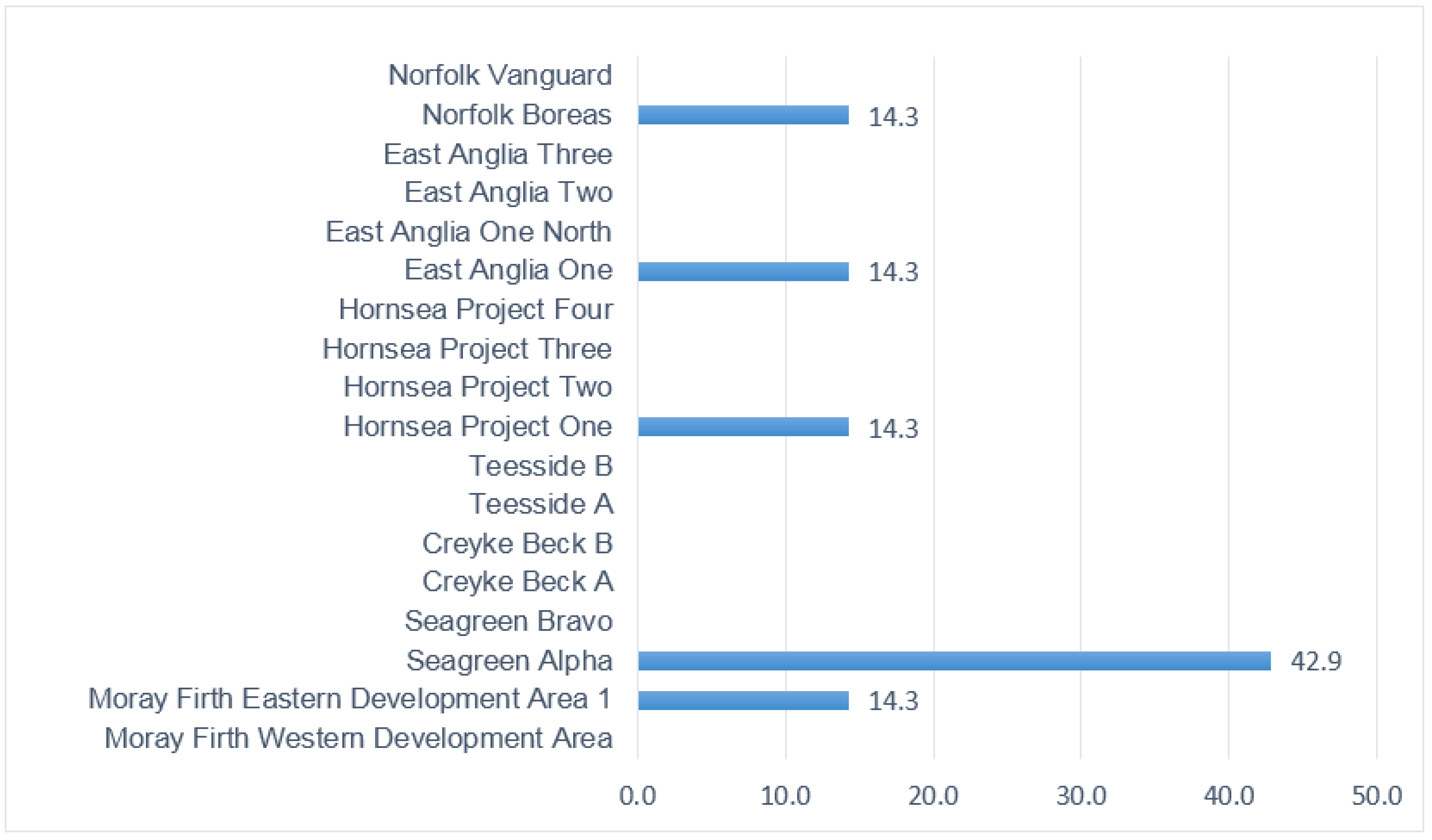Figure 10 illustrates the % frequency of the occurrences of the optimal solutions. Five locations were selected from the 18 in total. Seagreen Alpha was selected three times more than the rest of the optimum solutions.

The output of MOO is used as an input to the MCDM process. The output of TOPSIS is a prioritization of the alternatives (i.e., the five offshore sites). Two variations of TOPSIS (i.e., deterministic and stochastic) are employed. By combining those two methods, MOO and MCDM, the best location is identified, and the decision maker’s confidence increases. These five locations were selected to take part in the MCDM process in order to be further discussed and to obtain a ranking of the locations using the stochastic expansion of TOPSIS. Following the process of TOPSIS, the considered alternatives are listed in

Table 6. List of alternatives.

Alternatives/Zones	Wind Farm Site Name	ID
Moray Firth	Moray Firth Eastern Development Area 1	A1
Firth of Forth	Seagreen Alpha	A2
Hornsea	Hornsea Project One	A3
East Anglia (Norfolk Bank)	East Anglia One	A4
East Anglia (Norfolk Bank)	Norfolk Boreas	A5

, which are all considered to be unoccupied and available for a new wind farm installation for the purposes of the problem.

Table 7. Decision matrix.

Alternatives/Criteria	C1	C2	C3	C4	C5	C6	C7
A1	4.5	11.5	61,979,649,702	25.8	226	5.6	118.7
A2	4.5	10.4	31,984,700,386	25.8	157.5	6.4	129.2
A3	7	10.0	65,153,119,337	26.0	5939	6.4	114.2
A4	6	9.8	29,122,509,239	25.8	1859	6.7	114.5
A5	4.5	10.0	39,619,870,326	25.8	1859	6.7	114.2

shows the final decision matrix with the mean values for every alternative versus criterion. The criteria and alternatives’ IDs were used for clarity and simplification. All qualitative inputs were scaled from 1 to 9, as mentioned before.

Table 8. Frequency of experts’ preference per criterion.

Rate (1–5)	Criteria
	C1	C2	C3	C4	C5	C6	C7
1 Not at all important	0	0	0	0	0	0	0
2. Slightly important	1	1	5	1	1	0	1
3. Moderately important	5	1	3	6	2	5	1
4. Very important	4	7	2	2	6	7	4
5. Extremely important	3	4	3	4	4	1	7
Normalized mean weights	0.138	0.153	0.121	0.138	0.150	0.138	0.161

shows the frequency of the experts’ preference per criterion and the normalized mean values of the weights extracted from them.

Specifically for the calculation of C6 against alternatives in Table 7, input from three experts was considered. Although the number of experts replying to the seven criteria was mentioned before (i.e., 13), a different number of experts (i.e., 3) was involved in the estimation of the geotechnical condition criterion in order to form the distribution from their answers. The reason that the number of experts was not the same in the two procedures is that different expertise was required in both cases. The geotechnical conditions can be better perceived by geotechnical engineers, and the total number of experts is very specific and more difficult to engage with. Based on experts’ answers, the normalized mean weights of the criteria are estimated by the frequency of experts’ preferences per criterion in Table 8.

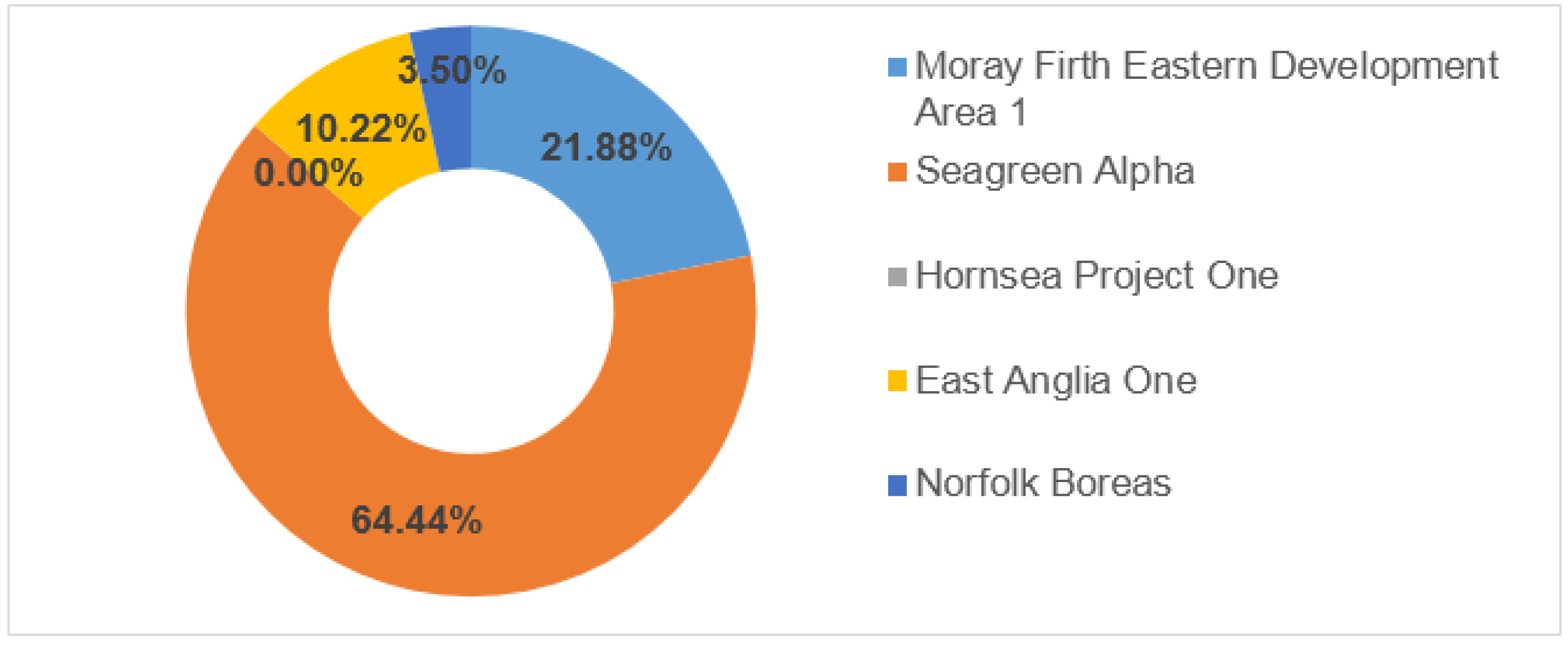
The results of both variations of TOPSIS are listed in

Table 9. Results of deterministic and stochastic Technique for the Order of Preference by Similarity to the Ideal Solution (TOPSIS).

Alternatives	Deterministic TOPSIS		Stochastic TOPSIS
	Score	Rank	Score	Rank
A1	0.733	2	21.88%	2
A2	0.816	1	64.44%	1
A3	0.181	5	0.00%	5
A4	0.712	3	10.22%	3
A5	0.660	4	3.50%	4

. By implementation, the stochastic variation reveals more quantitative information about the alternatives and assigns the probability that an option will rank first, as shown in Figure 11. According to stochastic TOPSIS, the alternative that involves Seagreen Alpha was the most probable solution, followed by Moray Firth Eastern Development Area 1. Also, the former is three times more probable to be selected compared to the latter. The probability of other options to be selected is significantly lower, and Hornsea Project One is unlikely to be selected.

In the survey, the experts were asked to make recommendations or leave comments about the criteria in order to include their insight in future studies or the limitations section. As expected, most experts made some recommendations that are worth considering in the next steps. Some experts responded according to their understanding of the work that is carried out and the work that was done before this study. Some of them pointed out factors that were already included in the study in the modelling of the work or already included in the criteria given to them, for example, the grid availability and the power prices.

The importance of the operational environmental conditions was pointed out and how critical they think it is as it drives the wind farm’s maximum output and capacity factor. It was also stated that the wind speed should be taken into account separately in the study. The geotechnical conditions and the soil’s impact on the design (both substructure and transmission system) were also pointed out. One expert made clear this should not be overlooked. The geotechnical conditions were studied separately and finally incorporated into this study as explained above.

At the end of the survey, the experts were asked to include any other criteria that can affect the location selection. One suggestion was to include the consenting process as it can be affected by environmental reasons such as the protection of biodiversity. This problem was seen in a wind farm due to Sabellaria reefs in the past. The ease and time of consent were also raised by another expert. It was suggested that specific stakeholders should be asked to participate such as the Ministry of Defence, air traffic, shipping, fishing, etc.

The government support mechanism came up in the comments a few times. It was also mentioned that the government regulations for each location need to be checked, because in many cases it might be a better decision to open the market in other continents. Also, the project financing and other contracts for difference (CfD) opportunities were mentioned. On top of that, the access to human resources was pointed out to show the impact of different locations.

Also, it was mentioned that if floating support structures were considered in the study, then the water depth and availability of relatively large and deep shipyards would be very important constraints. In this case, floating structures were not considered, but they could be included in the future.

The results of the study could also impact the criteria and the way these locations are selected by the Crown Estate providing more informed and cost-efficient options for future developers. Considerable actions are mandated on top of the development plans for minimizing investment, developing the supply chain, securing consents, ensuring economic grid investment and connection, and accessing finance [2,5].

5. Conclusions

The coupling of MOO with MCDM and expert surveys was demonstrated in this paper, as a method to increase the confidence of wind energy developers at the early stages of the investment. A set of locations from Round 3 and types of turbines were considered in the LCC analysis. By employing NSGAII and two variations of TOPSIS, optimum solutions were revealed and ranked based on experts’ preferences. In the current problem formulation, among the optimum solutions, Seagreen Alpha was the best option, and Hornsea Project One was the least probable to be selected. From the surveys, additional criteria and stakeholders were recommended by the participants, which will be considered in the future.

The proposed methodology could also be applied to other sectors in order to increase investment confidence and provide optimum solutions. For example, the installation of floating offshore wind and wave devices could benefit from the framework where the optimum locations can be suggested concerning cost and operational aspects of each technological need. The foundation in this study is considered to be the jacket structure because the LCC is formulated accordingly. More LCC parametric analyses can be investigated in the future for different types of structures.