Thermo–Economical Evaluation of Producing Liquefied Natural Gas and Natural Gas Liquids from Flare Gases

Abstract

In many industrial plants including petrochemicals and refineries, raw hydrocarbons (mostly flammable gas) are released during unplanned operations. These flammable gases (usually called flare gases) are sent to a combustor and the process is called flaring. Flaring wastes energy and produces environmental pollution. Consequently, recovering the flare gases is an important subject in these industries. In this work, an economical and technical analysis is presented for the production of valuable products, namely, liquefied natural gas and natural gas liquids from flare gas. The flare gas of Fajr Jam refinery, a refinery located in the south part of Iran, is selected as a case study. One of the issues in recovering flare gases is the nonconstant flow rate of these gases. For this reason, an auxiliary natural gas flow rate is employed to have a constant feed for the flare recovery process. The Poly Refrigerant Integrated Cycle Operations (PRICO) refrigeration cycle is employed for producing liquefied natural gas and natural gas liquids. In the PRICO cycle, the mixed refrigerant is used as the working fluid. The other issue is the existence of H₂S in the flare gases. The main idea is that the flare gas components, including H₂S, have different boiling points and it is possible to separate them. Consequently, flare gases are separated into several parts during a number of successive cooling and heating stages and passing through phase separators. It is shown that the proposed flare gas recovery process prevents burning of 12 million cubic meters of the gases with valuable hydrocarbons, which is almost 70% of the current flare gases. Furthermore, about 11,000 tons of liquefied natural gas and 1230 tons of natural gas liquids are produced in a year. Finally, the economic evaluation shows a payback period of about 1.6 years.

1. Introduction

In recent years, the high emissions of greenhouse gases have caused environmental pollution and increased global concern. Petrochemicals and refineries are the main energy consumers that have a great share of greenhouse gas emissions. In these industries, large amounts of hydrocarbons are burned due to safety issues in the flares. A flare stack is a gas combustion device which is used in industrial plants such as petroleum refineries, chemical plants, and natural gas processing plants for burning unwanted and flammable gases. Studies have reported that in 2016, more than 149 billion cubic meters of gas was burned in flares in the world [1]. It represents a huge waste of energy and financial resources and an increase of about 2 billion cubic meters compared to 2015.

The mentioned explanations have led to research and proceedings to reduce flaring. The solid oxide fuel cell (SOFC) system for reducing flare gases was presented by M. Saidi et al. [2]. Based on the results obtained from this system, in addition to generating 1200 MW electrical energy, the amount of pollutant gas emissions reduced from 1700 kg/s to 68 kg/s. Sonawat et al. [3] showed that flare gas can be recovered using an ejector. The ejectors have been used to increase the pressure of flare gases by high-pressure motive fluids and then reinjecting them into the pipelines. They compared their work with other flare recovery systems and found that the ejector was the simplest and cheapest because of low initial cost, adaptability to changes in operating conditions, low operation and maintenance costs, high rate of return and short payback period (PBP). Studies on design parameters of the flare gas recovery system (FGRS) by Enayati et al. [4] was performed. Their simulations were done in steady state and dynamic conditions in order to compare these two modes. Their simulation results indicated that the recovery of 5916 (nm³/h) of sweet natural gas, 24 (ton/h) of gas condensates and production of 297 (m³/h) of acid gas would be possible. One of the recovery methods proposed by Zadakbar et al. [5] was to compress the flare gases and return them to the fuel gas header for immediate use as fuel gas. A feasibility study of a flare gas recovery system in a real refinery was carried out by Gabriel et al. [6]. Their work focused on the selection and design of the flare gas recovery system, the gas treatment and reuse, the economic feasibility, and finally the payback period of the system. Choosing a liquid ring compressor to recover flare gases showed the payback period was about 2.5 years. The separation of gas and oil phases remained the most important step in the so-called surface production. Mourad et al. [7] performed studies on optimal pressure stages in the separation process in order to reduce flaring. Xu et al. [8] conducted a study to reduce the flaring in the startup of a petrochemical unit. Their results showed that it would be possible to prevent wasting large quantities of volatile organic compounds (VOCs).

Anomohanran et al. [9] studied the environmental impacts from pollutant emissions of burning associated gases in flares. They concluded that flaring wasted 11 billion dollars annually. Abdulrahman et al. [10] examined the key role of the Clean Development Mechanism (CDM) to overcome the difficulties of gas flaring recovery projects in developing countries. CDM is one of the three market-based mechanisms adopted under the Kyoto Protocol.

Some researchers have also modeled several plans to recover flare gases from a unit. After economic analysis, they offer the most cost-effective model. Rahimpour et al. [11] proposed three strategies for recycling associated gases and preventing the release of pollutants to the environment, namely gas-to-liquid (GTL) process, electricity generation with a gas turbine, and compression and injection into the refinery pipelines. Finally, the results of their research showed that generating electricity from these flare gases is more cost-effective than the two others. Banwarth et al. [12] provided detailed explanations into the design of one-stage and two-stage compressors used in flare gas recovery plants. Zolfaghari et al. [13] presented three models for the utilization of flare gases and their optimal use. These three ways included gas to liquid (GTL), gas turbines generation (GTG) and gas to ethylene (GTE). They concluded that the GTG method has the most economic benefits.

Also, some chemical methods have been proposed to reuse the flare gases by now. M. Beal et al. [14] investigated the energy return on investment (EROI) of the synergistic integration of flare gas with a microalgae biorefinery. They proposed a method to utilize flare gas for production of biofuel and protein from alga which indicated a beneficial system environmentally. Moreover, integration and reuse of flared gases with fuel gas network (FGN) is an impressive method for reducing greenhouse gas (GHG) emissions in addition to saving energy in refineries. An FGN model was modified by Tahouni et al. [15] and results indicated a 12% reduction in natural gas consumption compared to the nonintegrated flare gas stream case and a 27.7% reduction compared to the base case with no FGN. One of the drawbacks with the flaring is measuring the conditions of gas flaring. Heidari et al. [16] measured these conditions in a real gas refinery plant and they suggested two feasible structures for electrical power generation from the flare gas as two scenarios. The first scenario is burning the mixture of the flare gas and a conventional fuel, and the second one is sending the flare gas to an intermediate stage of a gas turbine after burning it in a combustor. The results showed that the first scenario is superior from technical and economic aspects.

In the present study, a flare gas recovery process is designed, simulated, and optimized in powerful ASPEN PLUS software (version 8.6, Aspen Technology Inc., Bedford, MD, USA). A thermo–economic analysis has been carried out for recovering valuable products (liquefied natural gas and natural gas liquids) from flare gases. Liquefied natural gas (LNG) is widely accepted as a clean energy alternative to other fossil fuels where natural gas (NG) is not available through pipelines [17]. Natural gas liquids (NGLs) are flammable mixtures consisting of light hydrocarbon products (ethane, propane, isobutane, pentane and some heavier species). 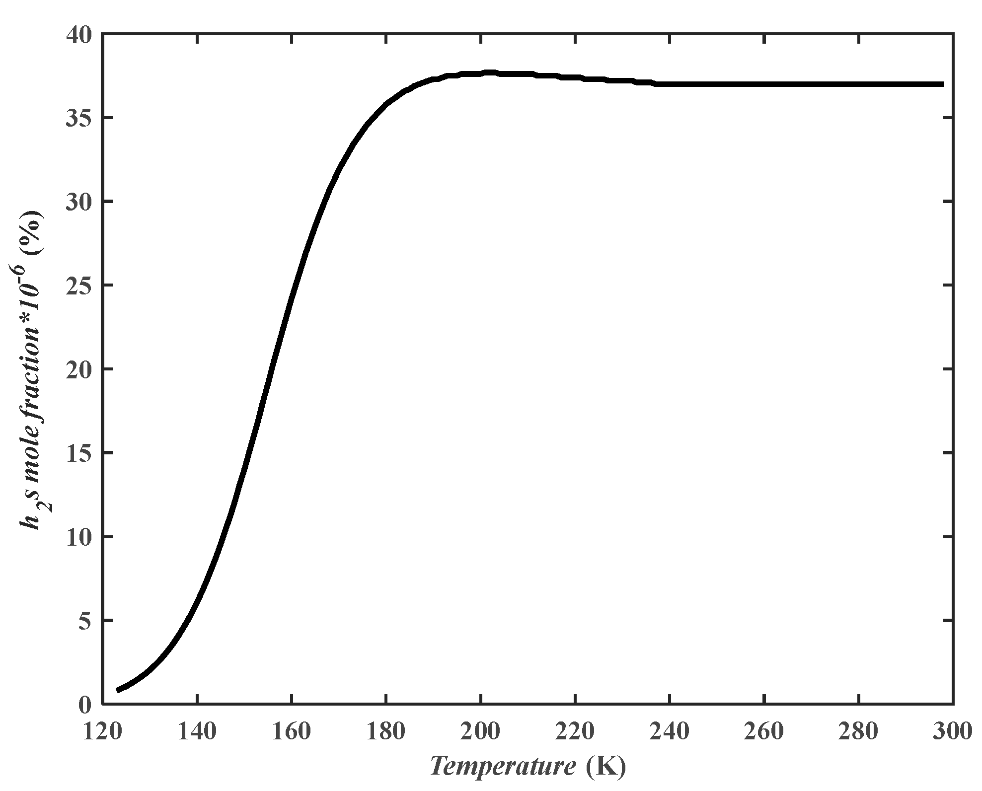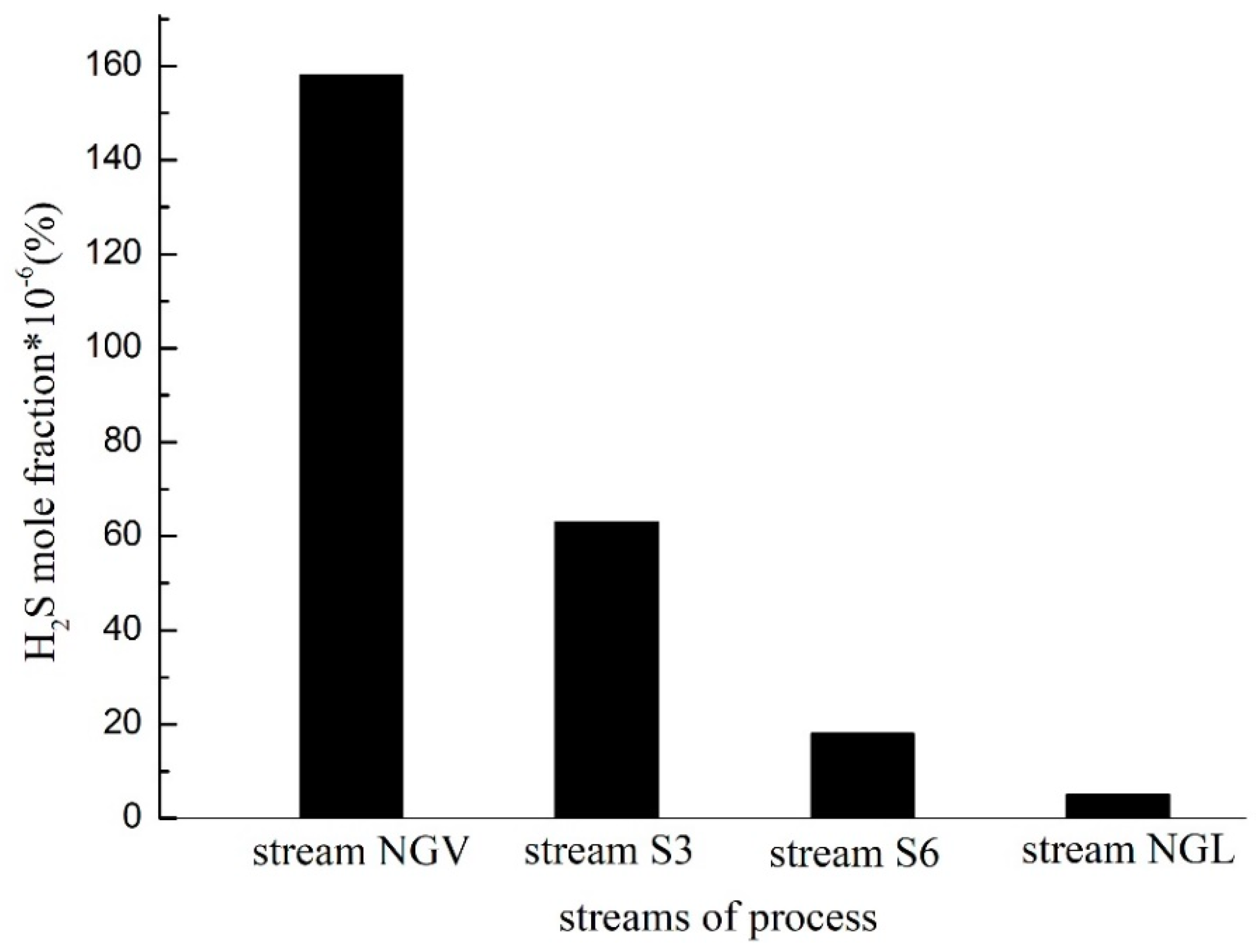NGL has a variety of applications and is mainly used for heating appliances, cooking equipment, vehicles and in the chemical industry [18]. In this study, the flare gases of the Fajr Jam refinery were selected as a case study. The most important issues were a nonconstant flow rate and an excessive H₂S in flare gas components. In refiners, removing H₂S usually is done by installing amine towers, but using this technology for low feed gas is not economically and technically justifiable. 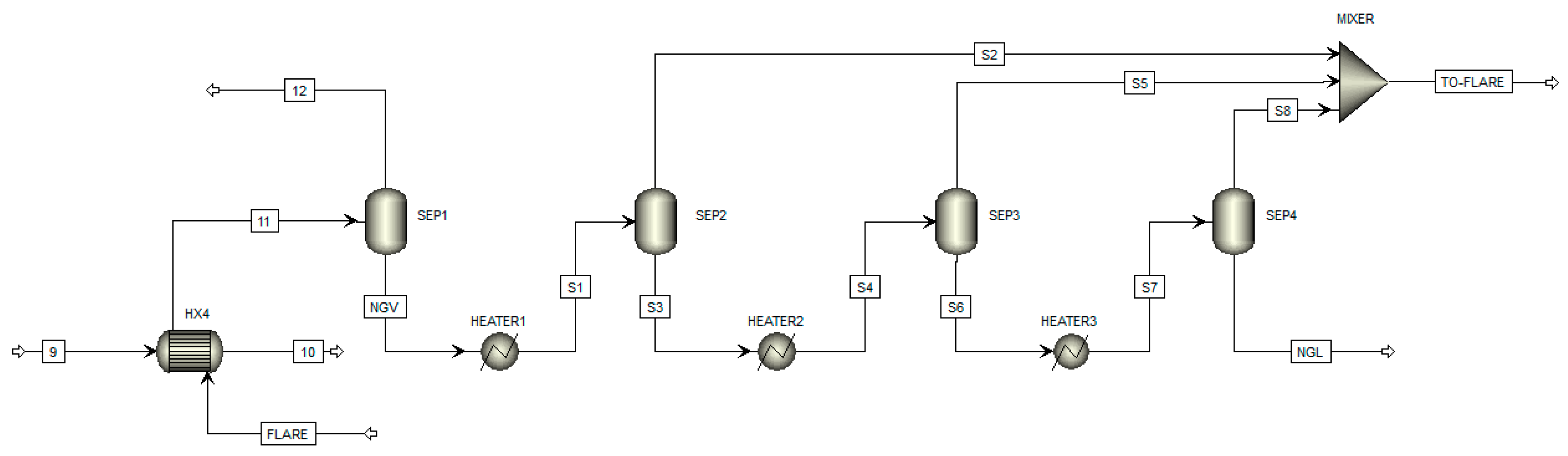In this work, the amount of H₂S in products (LNG and NGL) is reduced to a standard level with the help of a refrigeration cycle and the nonconstant flare gas flow rate issue is addressed with the help of an auxiliary flow to keep the feed flow rate constant. The flare recovery process is designed with three goals: separation of H₂S from gas flare, LNG, and NGL production.

2. Process Description

In this work, the data of the flaring system in the Fajr Jam refinery is used to design a flare recovery process. The process is divided into two main parts, namely, LNG and NGL recovery, as well as a refrigeration cycle.

2.1. Refrigeration Cycle and LNG Recovery

The technologies of refrigeration processes for the production of LNG are limited under the license and its owners. The differences between refrigeration cycles are in the type of refrigerant used, pure or mixed, the number of cooling cycles, the type of heat exchangers and the amount of production capacity. Due to the low flow rate of flare gases and also standard engineering design packages for the “Mid-small-mini Scale LNG Plant” (production capacity of 0.1–1.5 million tons per year [19]), the PRICO (Poly Refrigerant Integrated Cycle Operations) cycle could be a good candidate. The other technologies for liquefying natural gas (like cascade, propane pre-cooled mixed refrigerant (C3MR), dual mixed refrigerant (DMR), etc.) need a lot of equipment and this makes them more expensive. After analyzing and considering the flare gas conditions such as flow rate, temperature, pressure, and so on, the PRICO cycle is selected for the cooling process. It is also known as a single mixed refrigerant (SMR) process. This cycle has several advantages such as a low amount of required equipment, a relatively simple process, low capital and operating cost, high flexibility, high reliability, and rapid startup [20].

The flow diagram of the PRICO cycle is illustrated in Figure 1. The working fluid (refrigerant) is assumed as a mixture of methane, ethane, butane, and nitrogen. In this process, the pressure of the mixed refrigerant is increased after passing through the compressor. Then, its temperature is reduced by passing through the condenser as a constant-pressure process. Subsequently, by passing gas from a multistream heat exchanger, approximately constant pressure, its temperature is greatly reduced and then it is passed through a throttle valve to decrease its temperature and pressure. The flow with low pressure and low temperature re-enters the heat exchanger to provide the cooling needed for the liquefaction of natural gas.

Figure 2 shows a schematic representation of the desired PRICO cycle. The difference between this cycle and the previous cycle is the existence of a hot stream in the multistream heat exchanger. Therefore, stream 5 returned again to the heat exchanger in order to cool the three streams 3, 8 and flare. Hence, the flare gas initially is cooled down slightly and then the liquid and gas phases are separated from each other in a separator. This cycle has a four-stream heat exchanger. Generally, a plate fin heat exchanger is constructed to do this duty. By simulating this type of multistream heat exchanger with a software’s built-in model, the software only carries out the overall mass and energy balance. Hence, examining these results for the temperature cross may not result in the correct answer, because the software’s built-in model for a multistream heat exchanger does not check the temperature cross and the feasibility of its result. Therefore, the heat transfer needs of the process are met through an equivalent heat exchanger network [21]. On the other hand, the minimum number of two-stream heat exchangers needed to fulfill the thermal duty of the process is calculated from N–1, where N is the total number of process streams [21,22]. Owing to the fact that there are four process streams, with the three heat exchangers the thermal duty of the process is satisfied. Therefore, the problem of the shortage of software’s built-in model is solved with the replacement of a multistream heat exchanger model with the equivalent network of the three models of the two-stream heat exchanger. So, the mass and energy balances are carried out and at the same time, any temperature cross is avoided. Finally, the refrigeration cycle diagram of the flare recovery process is changed, as shown in Figure 3.

Due to the difference in the boiling points of different gas components, the cooling process could liquefy some of the flare gas components. Figure 4 shows the changes of H₂S mole fraction in stream 8 of Figure 2 with the temperature in the cooled flare gas stream (stream 6 in Figure 2). With decreasing the temperature, the gas becomes two-phase and the H₂S mole fraction reduces in the vapor phase. In this cycle, at first, flare gas is cooled to 138.5 K. This temperature is selected because of the allowed amount of H₂S (<4 ppm) [23] in the gas phase. Higher quantities of H₂S (>4 ppm) cause gas poisoning. The gas phase, stream 8 in Figure 2, which includes 96% of methane and an allowable amount of H₂S, returns to the heat exchanger for liquefaction. The H₂S mole fraction in the NGV stream in Figure 2, which is in the liquid phase, is not in the allowed range. So, it is sent to the next step of the process for NGL recovery and H₂S correction.

According to Figure 3, it could be seen that from stream 1 to stream 5, after the throttle valve, the cycle is similar to the previous cycle in Figure 2. After this stream, the flow is divided into two parts. The first one is stream 6 and its task is to cool the refrigerant before entering the throttle valve. The second one is stream 8 that enters the HX3 and HX4, where methane is liquefied and is separated with allowed H₂S amounts. Streams 10 and 7 are combined in a mixer to form stream 1 and return to the compressor. The following assumptions were considered for the simulation: The ambient temperature is 298 K, the ambient pressure is 1.013 bar, the pressure drop within the heat exchanger is assumed zero [24], and the isentropic efficiency of the compressor is assumed 80% [20]. The compositions of refrigerant and flare gas are given in

Table 1. Compositions of flare gas, natural gas, and refrigerant.

Composition (mol %)	Flare Gas	Natural Gas	Refrigerant
N2	2.33	0.22	0.2
CO2	0.0076	0	0
H2S	0.0037	0	0
C1	76.88	95.33	0.26
C2	11.41	2.36	0.28
C3	4.66	1.14	0
I-C4	0.97	0.46	0
N-C4	1.38	0.47	0.26
I-C5	0.61	0.01	0
N-C5	0.43	0.01	0
C6	0.37	0	0
C7+	0.19	0	0

.

The simulation data are given in

Table 2. Specifications of cycle in Figure 3.

Stream	T (K)	P (bar)	m (kg/h)
1	288	1	55,000
2	442	48	55,000
3	313	48	55,000
4	103	48	55,000
5	96.5	1	55,000
6	96.5	1	44,000
7	304	1	44,000
8	96.5	1	11,000
9	114	1	11,000
10	147	1	11,000
11	138.5	1	2100
12	138.5	1	1285.27
13	138.5	1	813/29
Air1	298	1	131,000
Air2	394.72	1	131,000
Flare	298	1	2100
LNG	103	1	1285.27

.

2.2. NGL Recovery

This section describes the process of separating H₂S and NGL from the remaining flare gas, that is, stream NGV in Figure 3. This process is based on the difference in boiling point of various flare gas components which are indicated in

Table 3. Boiling points of flare gas components.

Component	T (K)
C1	109
C2	184
C3	231
C4	272.5
C5	309
C6	342
C7	371
N2	77.2
H2S	213
CO2	194.5

[25].

In general, NGV 13 in Figure 5 (which corresponds to the stream NGV in Figure 3) is heated in several steps and passes through a separator in every step. So, in the final step, its hydrogen sulfide meets the allowable amount. To better understand this, a schematic of this process is shown in Figure 5. At first, the stream NGV, which is in the liquid phase, is slightly heated and partially vaporized. This makes hydrogen sulfide go to the vapor phase and after passing through the separator, its amount in the liquid phase reduces. This process occurs three times in a successive manner to make the concentration of H₂S in the liquid phase 4 ppm. Figure 6 illustrates the hydrogen sulfide mole fraction changes in the liquid phase from stream NGV to stream NGL.

The temperatures of streams 11, S1, S4, and S7 have been determined by software optimization. For this purpose, the total mass flow rate of LNG and NGL streams are selected as an objective function and constraints are the H₂S amount in these streams, which should be less than 4 ppm. For energy optimization in this part of the cycle, the inlet flare gas was used to heat the streams NGV, S3 and S6. After designing both parts of the flare recovery process, the heat integration of the entire process is performed.

3. Process Simulation and Optimization

3.1. Simulation Method

With combination of the two parts of the process (Figure 4 and Figure 5), the final flare recovery process is shown in Figure 7. Aspen PLUS software with the Sequential Modular method (SM method) and the Penge–Robinson equation of state are used for simulation of the process. The key factor is the amount of flare that varies during the year. However, the process requires a steady flow rate. Therefore, a constant amount (monthly average flaring per year) was considered and the amount of feed shortage is offset by refined gas from the refinery outlet. So by installing a control system, the flare flow rate fluctuations could be covered. On the other hand, when the associated gas flow rate is too much for the cycle, extra gases will be sent to the flare.

Thermal integration is performed by Aspen Energy Analyzer and then its results are transferred to the ASPEN PLUS software. The composite curves of the heat exchanger network and the temperature approach of the flare recovery process are indicated in Figure 8.

3.2. Optimization Method

The results of the SM method are used as the initial estimations in the Equation-Oriented method (EO method). These basic estimations include: the mole fractions of the refrigerant components, pressure level, refrigerant flow rate, and the pressure after throttle valve. Finally, the EO method is used in the process optimization. The problem of achieving optimal operation can be formulated as:

$$\{\begin{array}{c}\underset{u}{\min }{W}_s\\ \mathrm{subject} \mathrm{to}: f\left(x\right)=0\end{array},$$

(1)

where W_s is the work of the compressor, which is the objective function of the optimization problem, and u is the vector of adjustable input variables. This is a six-element vector and includes the pressure increase imposed by the compressor, mole fraction of methane, ethane, n-butane, nitrogen in refrigerant, and the flow rate of refrigerant. The function f(x) represents the plant model.

To solve this optimization problem, the large-scale sparse successive quadratic programming (LSSQP) algorithm is used. This algorithm is a variant of a class of successive quadratic programming (SQP) to solve large-scale optimization problems. It performs the optimization by solving a sequence of quadratic programming subproblems. The main parameter of this method is as the

Table 4. Parameters of the optimization method (successive quadratic programming (SQP)).

Parameter	Description	Value
Relative convergence tolerance	It is used in the Kuhn–Tucker error criterion	0.0001
Maximum iterations	The maximum number of (SQP) iterations allowed.	50
Iteration-constraint violation	The maximum number of feasibility corrections allowed at each SQP iteration to try to keep constraint violations below the iterative constraint violation tolerance.	2
Iteration-constraint violation tolerance	The limit above which feasibility correction will be applied after every iteration.	0.01
Final-constraint violation tolerance	The limit above which feasibility correction will be applied at the end of the optimization calculation.	1 × 10−6

:

3.3. Simulation and Optimization Results

The objective function of the optimization problem is the compressor’s work reduction. An important point which should be considered is to determine the temperature of the inlet and outlet of heat exchangers to prevent the temperature cross. By optimizing the refrigerant’s composition, the total work of the compressor is also reduced, because the flow rate and the pressure level of the process are reduced with changing refrigerant mole fraction. The optimization results are listed in

Table 5. Results of optimization.

Variable	Before Optimization	After Optimization
Flow rate (kg/h)	55,000	36,100
Pressure level (bar)	1–48	1.19–38
Compressor work (kW)	6500	3300

.

4. Economical Evaluation

In this section, the capital costs of the flare recovery system are determined and then an economical evaluation is conducted. Various methods can be used to estimate investment costs. Selection of each method depends on the available information and accuracy. In this research, the percentage of equipment prices method is used [26]. This method is used to estimate the total investment cost and it needs the price of equipment in the process. Other items in the total direct cost of the plant are also estimated with the use of a percentage of this cost. So, at first, the cost of the process equipment is calculated, then other costs are obtained. To calculate the price of equipment, except compressor, Equation (2) is used [27]:

$$lo{g}_{10}{C}_P^0=K_1+K_{2}lo{g}_{10}\left(A\right)+K_3{\left[lo{g}_{10}\left(A\right)\right]}^2,$$

(2)

where $C_P^0$ is the equipment price, A the capacity or measurable parameter for equipping, and $K_1$, $K_2$ and $K_3$ are constants [28].

Because of the capacity of the compressor, Equation (2) is not suitable. So Equation (3) is used to calculate the compressor price [29].

$$PE{C}_{ac}=\left[\frac{C_{11}{m}_a}{C_{12}-{\eta }_{sc}}\right]\times \left(\frac{P_2}{P_1}\right)ln\left(\frac{P_2}{P_1}\right),$$

(3)

where $P_1$ and $P_2$ are the inlet and outlet pressure of the compressor, respectively, ${\dot{m}}_a$ is the flow rate (kg/s), ${\eta }_{sc}$ is the compressor’s isentropic efficiency, and $PE{C}_{ac}$ is the cost of the compressor. The calculated prices are shown in

Table 6. Cost estimation of flare recovery equipment.

Component	Compressor	Heat Exchangers	Separators	Total
Cost (Dollars)	812,447	618,976	58,400	1,489,823

.

The assumptions used in the economic evaluation model, in order to estimate the time of return on investment, are shown in

Table 7. Assumptions considered in the economic analysis [30].

Row	Content	Amount
1	Tax rate (%)	0
2	Interest charge	12
3	Price per cubic meter of natural gas (dollars)	0.065
4	Price increase per cubic meter of natural gas (%)	8
5	The price of LNG (dollars/kJ)	0.85 × 10−5
6	The price of NGL (dollars/kJ)	0.67 × 10−5
7	LNG increase rate (%)	3
8	NGL increase rate (%)	3
9	Cost of electricity (dollars/kWh)	0.017
10	Increase in kilowatt hours of electricity (%)	8
11	Annual unit operation (hours)	7992
12	Lifetime of the system (year)	20

. The required investment to build each unit includes direct and indirect investment costs.

The relative factors for estimating direct and indirect investment costs based on the equipment price of the processing units are shown in

Table 8. Fixed capital investment costs [26].

Components	Assumed % of Total	Cost (Dollars)	Rationed % of Total
Purchased equipment	30	1,489,823.0	27.52
Purchased equipment installation	10	496,607.7	9.17
Instrumentation and controls (installed)	6	297,964.6	5.50
Piping (installed)	12	595,929.2	11.0
Electrical (installed)	3	148,982.3	2.75
Buildings (including services)	8	397,286.1	7.33
Yard improvement	2	99,321.5	1.83
Service facilities (installed)	8	397,286.1	7.33
Engineering and supervision	10	496,607.7	9.17
Construction expense	9	446,946.9	8.25
Contractor’s fee	3	148,982.3	2.75
Contingency	8	397,286.1	7.33
Total	-	5,413,024.0	100

. Variable costs are those which vary directly with the output of a particular plant or production process, such as fuel costs [30].

Table 9. Costs and incomes.

Component	Electricity	Labor	Maintanence	NG	LNG	NGL
Annual requirement for the operation of the process	26,373,600 (kWh/annum)	731 (workers·shift/year)	-	5,500,000 (SCM/year)	-	-
Annual operating cost (dollars/year)	450,280	146,200	104,287	355,487	-	-
Production per year (kg/year)	-	-	-	-	11,274,401	1,569,026
Income (dollars/year)	-	-	-	-	4,506,726	504,566

shows the annual income and the cost of fuel before starting the plant. Based on the fixed and variable costs, analysis is done. To calculate payback period, the net present value (NPV) method is used.

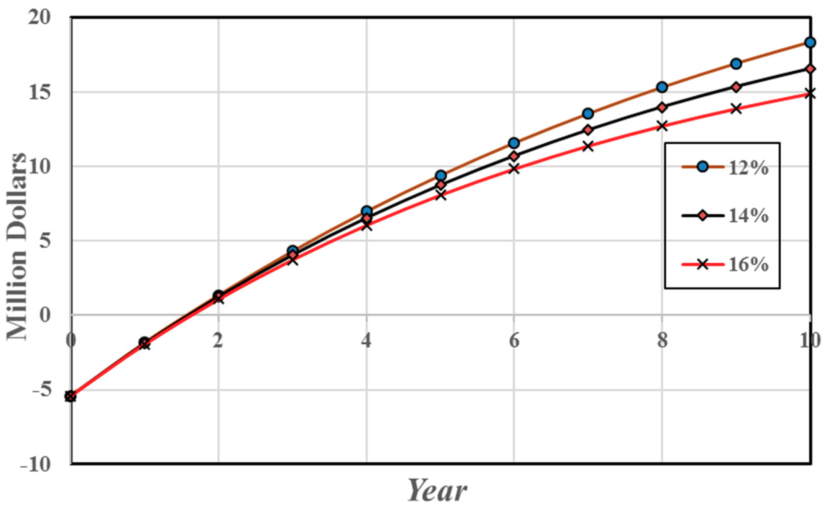
The NPV method calculates and summates the present value of all the annual cash flows that have been achieved or consumed over the life of the project. Costs are considered to be in the form of negative values and incomes as positive values. The sum of all the present values is known as the NPV. The discount factor is based on an assumed discount rate, that is, interest rate, and can be determined by using Equation (4).

$$DF={\left(1+\frac{IR}{100}\right)}^{-n},$$

(4)

where $DF$ is discount factor, $IR$ is the interest rate, and $n$ is the time period.

The NPV is calculated for the three discount rates of 12%, 14%, and 16%. From Figure 9, the payback period can be calculated. If a line from the zero point from the vertical axis and parallel with the horizontal axis is plotted, it will cross the curves at a point where it shows the time of returning the capital cost. This zero line is shown in Figure 9. This value is 1.6 years for almost all discount rates.

By utilizing the proposed flare recovery process, about 12 million cubic meters of flare gas are estimated to be saved yearly. In addition, with the proposed flare gas recovery process, annual production of more than 11 thousand tons of LNG and annual production of over 1230 tons of NGL are possible.

5. PRICO Cycle Validation

Unfortunately, the results of the optimal conditions cannot be directly compared with other papers that use the PRICO process. Small variations in conditions such as scale, flow rates of NG and MR, NG composition and efficiency of heat exchangers have large impacts on process results. However, the optimal conditions can be compared to show that the results are in accordance with those found in the literature. It is clear from

Table 10. Comparison of optimal refrigerant compositions.

Paper	Hatcher et al. [31]	Jensen and Skogestad [32]	Nogal et al. [28]	Lee et al. [33]	Aspelund et al. [34]	This Study
Composition—nitrogen, mol %	7.3	8.2	10.1	11	10.5	15.5
Composition—methane, mol %	36.1	31.9	27.1	27.3	26.9	28.8
Composition—ethane, mol %	48.8	35.2	37.2	35.6	37.6	25.7
Composition—propane, mol %	0	0	0.3	5.2	2.3	0
Composition—n-butane, mol %	7.7	24.7	25.3	20.9	22.7	28.9

that the results of the proposed flare recovery process are reasonable in comparison with the data available in the literature. Similarities are also found between the composition, particularly with a comparison of the optimal results achieved in this paper with optimal results found in the literature.

6. Alternative Process: Power Generation

The other alternative method for energy recovery of flare gases is the electricity generation process. The flare gas is burned in the boiler with 20% excess air to produce high-pressure (HP) steam at 25 bar. By letting down the HP steam through a turbine, electric power could be generated. The flowsheet of the process is as shown in Figure 10.

The combustion process in the boiler is modeled with the RGibbs reactor in the Aspen PLUS software. The RGibbs model uses the Gibbs free energy minimization technique to determine the composition of each phase. The mechanical efficiency of the steam turbine is considered to be 70 percent [26]. The fixed capital investment of the power generation process is as shown in

Table 11. Fixed capital investment costs [27].

Component	Cost (Dollars)
Pump	7600
Turbine	267,150
Boiler	2,340,000
Total	2,614,750

.

The value of generating electricity is 854,025 dollars/year and the payback period is calculated to be 3.06 years. So, the payback period of the power generation process is nearly twice the value of the payback period of the proposed method in this study. The advantage of the proposed process in this study will be more highlighted if the thermal efficiency of the boiler, operating cost of the power generation process, or nonmanufacturing fixed capital investments costs like engineering and supervision of the power generation process are included.

7. Conclusions

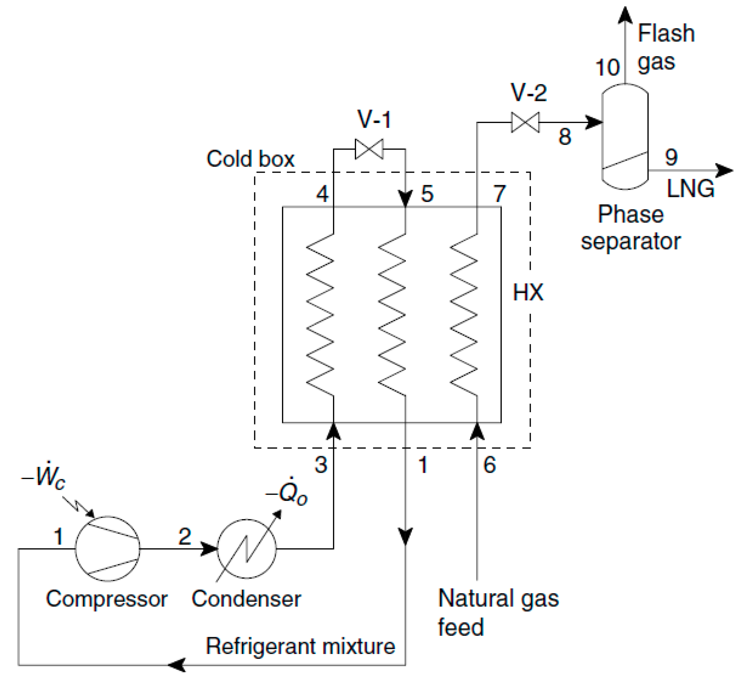
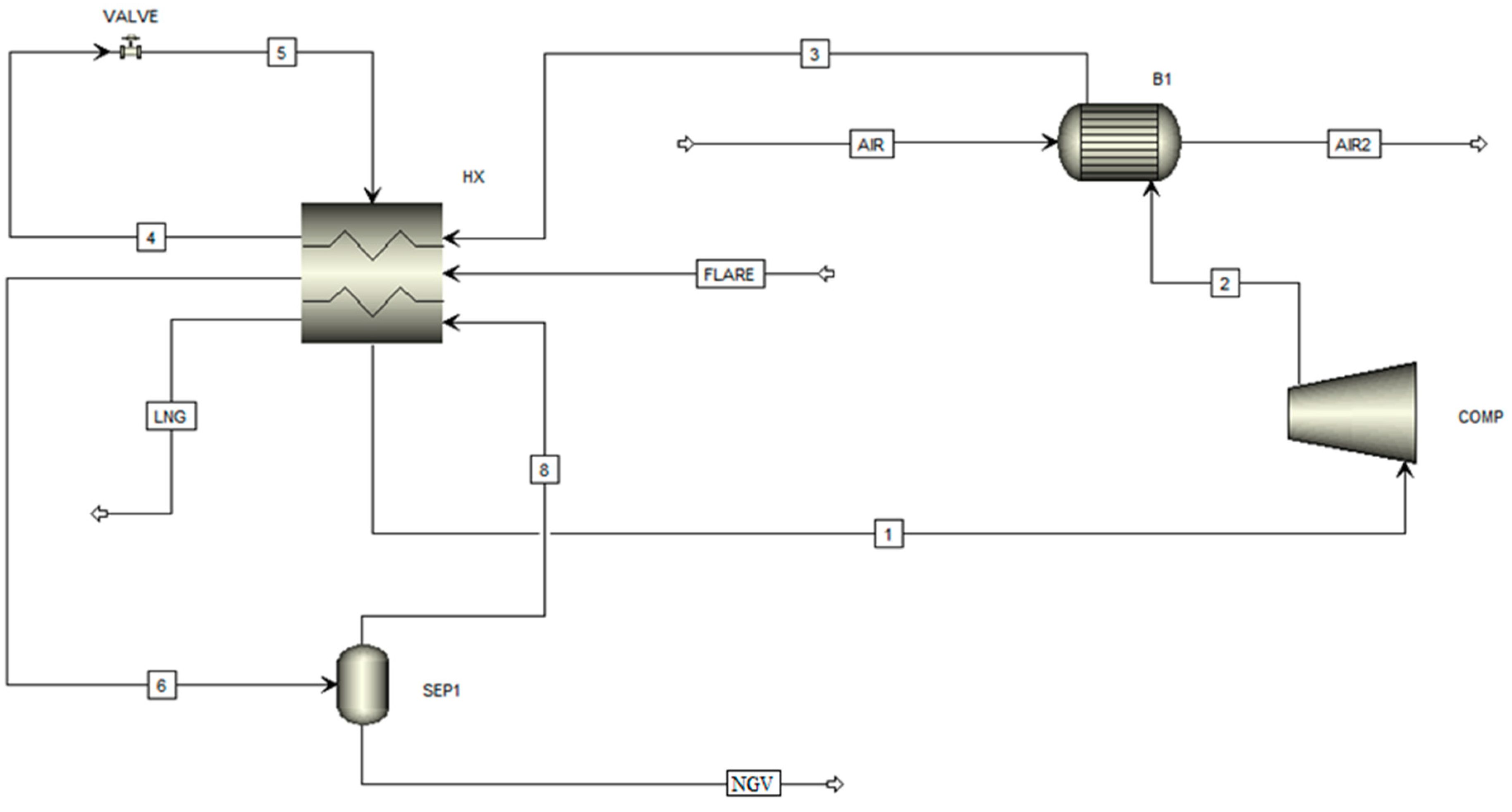
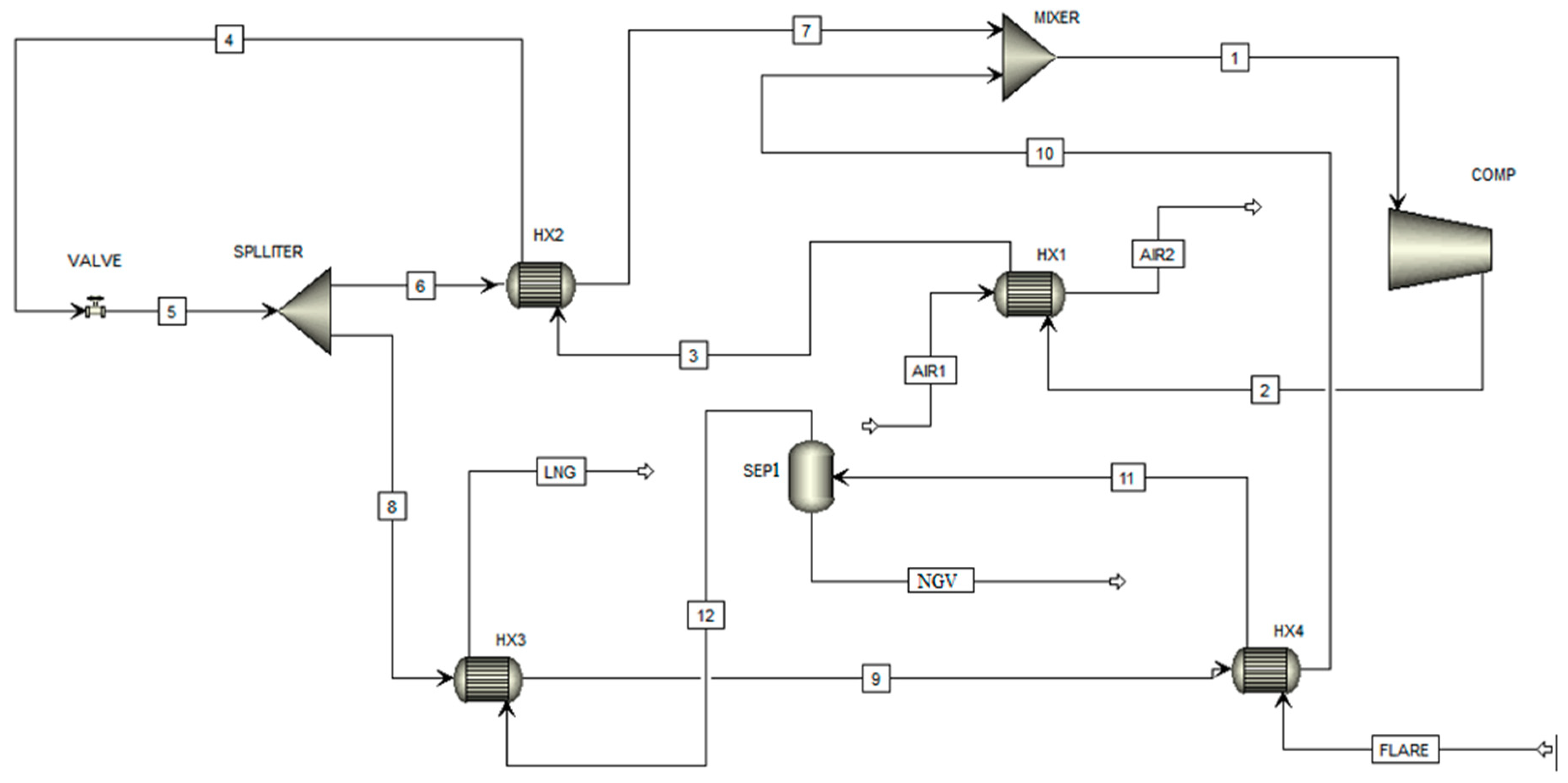
Attention to the environment and the value of preserving primary resources are the two factors which make it necessary to minimize flaring in accordance with practical considerations and constraints. Therefore, according to the environmental pollution and considering the added value that is completely eliminated, it is very logical to check the establishment of a unit for the recycling of flare gases and the production of valuable products from them. In this research, we tried to design a flare gas recovery system with consideration of the refinery’s normal conditions. In this process, a cooling cycle was used to reduce the H₂S level of flare gases and also separate LNG and NGL from it. Therefore, by selecting the Fajr Jam refinery flare gases as a case study, the process of producing gas condensate was designed. The PRICO cycle was used for the cooling process. Due to the design conditions, this refrigeration cycle undergoes some changes to improve the process. The results of simulation and economic analysis include:

• Avoiding the loss of about 12 million cubic meters of gas per year.
• Annual production of more than 11 thousand tons of LNG.
• Annual production of over 1230 tons of NGL.
• Payback period is about 1.6 years by using the net present value method.

Consequently, by applying the presented flare gas recovery process, both environmental and economic advantages could be achieved.

References

1. New Data Reveals Uptick in Global Gas Flaring. Available online: http://www.worldbank.org/en/news/press-release/2016/12/12/new-data-reveals-uptick-in-global-gas-flaring (accessed on 7 September 2017).
2. Saidi, M.; Siavashi, F.; Rahimpour, M. Application of solid oxide fuel cell for flare gas recovery as a new approach; a case study for Asalouyeh gas processing plant, Iran. J. Nat. Gas Sci. Eng. 2014, 17, 13–25. [Google Scholar] [CrossRef]
3. Sonawat, A.; Samad, A. Flare gas recovery using ejector-a review. In Proceedings of the Thirty Ninth National Conference on Fluid Mechanics and Fluid Power, Surat, Gujarat, India, 13–15 December 2012. [Google Scholar]
4. Sangsaraki, M.E.; Anajafi, E. Design criteria and simulation of flare gas recovery system. In Proceedings of the International Conference on Chemical, Food and Environment Engineering (ICCFEE’15), Dubai, UAE, 11–12 January 2015. [Google Scholar]
5. Zadakbar, O.; Vatani, A.; Karimpour, K. Flare gas recovery in oil and gas refineries. Oil Gas Sci. Technol. Rev. IFP 2008, 63, 705–711. [Google Scholar] [CrossRef]
6. Comodi, G.; Renzi, M.; Rossi, M. Energy efficiency improvement in oil refineries through flare gas recovery technique to meet the emission trading targets. Energy 2016, 109, 1–12. [Google Scholar] [CrossRef]
7. Mourad, D.; Ghazi, O.; Noureddine, B. Recovery of flared gas through crude oil stabilization by a multi-staged separation with intermediate feeds: A case study. Korean J. Chem. Eng. 2009, 26, 1706–1716. [Google Scholar] [CrossRef]
8. Xu, Q.; Yang, X.; Liu, C.; Li, K.; Lou, H.H.; Gossage, J.L. Chemical plant flare minimization via plantwide dynamic simulation. Ind. Eng. Chem. Res. 2009, 48, 3505–3512. [Google Scholar] [CrossRef]
9. Anomohanran, O. Determination of greenhouse gas emission resulting from gas flaring activities in Nigeria. Energy Policy 2012, 45, 666–670. [Google Scholar] [CrossRef]
10. Abdulrahman, A.O.; Huisingh, D.; Hafkamp, W. Sustainability improvements in Egypt’s oil & gas industry by implementation of flare gas recovery. J. Clean. Prod. 2015, 98, 116–122. [Google Scholar]
11. Rahimpour, M.R.; Jokar, S.M. Feasibility of flare gas reformation to practical energy in Farashband gas refinery: No gas flaring. J. Hazard. Mater. 2012, 209, 204–217. [Google Scholar] [CrossRef] [PubMed]
12. Bannwarth, H. Liquid Ring Vacuum Pumps, Compressors and Systems: Conventional and Hermetic Design; John Wiley & Sons: Hoboken, NJ, USA, 2006. [Google Scholar]
13. Zolfaghari, M.; Pirouzfar, V.; Sakhaeinia, H. Technical characterization and economic evaluation of recovery of flare gas in various gas-processing plants. Energy 2017, 124, 481–491. [Google Scholar] [CrossRef]
14. Beal, C.M.; Davidson, F.T.; Webber, M.E.; Quinn, J.C. Flare gas recovery for algal protein production. Algal Res. 2016, 20, 142–152. [Google Scholar] [CrossRef]
15. Tahouni, N.; Gholami, M.; Panjeshahi, M.H. Integration of flare gas with fuel gas network in refineries. Energy 2016, 111, 82–91. [Google Scholar] [CrossRef]
16. Heidari, M.; Ataei, A.; Rahdar, M.H. Development and analysis of two novel methods for power generation from flare gas. Appl. Therm. Eng. 2016, 104, 687–696. [Google Scholar] [CrossRef]
17. Eiksund, O.; Brodal, E.; Jackson, S. Optimization of Pure-Component LNG Cascade Processes with Heat Integration. Energies 2018, 11, 202. [Google Scholar] [CrossRef]
18. Wu, X.; Li, C.; He, Y.; Jia, W. Dynamic Modeling of the Two-Phase Leakage Process of Natural Gas Liquid Storage Tanks. Energies 2017, 10, 1399. [Google Scholar] [CrossRef]
19. Kunert, S.; Larsen, D. Small is beautiful–Mini LNG concept. In The Potential of Bio-Energy for Future Energy Supply; Hamworthy Gas System AS: Lipzig, Germany, 2008. [Google Scholar]
20. Morosuk, T.; Tesch, S.; Hiemann, A.; Tsatsaronis, G.; Omar, N.B. Evaluation of the PRICO liquefaction process using exergy-based methods. J. Nat. Gas Sci. Eng. 2015, 27, 23–31. [Google Scholar] [CrossRef]
21. Picon-Nunez, M.; Polley, G.; Medina-Flores, M. Thermal design of multi-stream heat exchangers. Appl. Therm. Eng. 2002, 22, 1643–1660. [Google Scholar] [CrossRef]
22. Hoffman, T. Optimal Design of Heat Exchanger Network and Evaluation of Current Procedures. In Heat Exchangers: Design and Theory Sourcebook; McGraw Hill Book Co.: New York, NY, USA, 1974. [Google Scholar]
23. Foss, M.M. Interstate Natural Gas—Quality Specifications & Interchangeability. Ph.D. Thesis, Center for Energy Economics, Bureau of Economic Geology, University of Texas at Austin, Austin, TX, USA, 2004. [Google Scholar]
24. Marmolejo-Correa, D.; Gundersen, T. A comparison of exergy efficiency definitions with focus on low temperature processes. Energy 2012, 44, 477–489. [Google Scholar] [CrossRef]
25. Timmis, K.N.; McGenity, T.; van der Meer, J.R.; de Lorenzo, V. Handbook of Hydrocarbon and Lipid Microbiology; Springer: Berlin, German, 2010. [Google Scholar]
26. Peters, M.S.; Timmerhaus, K.D.; West, R.E.; Timmerhaus, K.; West, R. Plant Design and Economics for Chemical Engineers; McGraw-Hill: New York, NY, USA, 1968. [Google Scholar]
27. Turton, R.; Bailie, R.C.; Whiting, W.B.; Shaeiwitz, J.A. Analysis, Synthesis and Design of Chemical Processes; Pearson Education: New York, NY, USA, 2008. [Google Scholar]
28. Nogal, F.D.; Kim, J.K.; Perry, S.; Smith, R. Optimal design of mixed refrigerant cycles. Ind. Eng. Chem. Res. 2008, 47, 8724–8740. [Google Scholar] [CrossRef]
29. Bejan, A.; Tsatsaronis, G. Thermal Design and Optimization; John Wiley & Sons: Hoboken, NJ, USA, 1996. [Google Scholar]
30. Beggs, C. Energy: Management, Supply and Conservation; Routledge: Abingdon-on-Thames, UK, 2010. [Google Scholar]
31. Hatcher, P.; Khalilpour, R.; Abbas, A. Optimisation of LNG mixed-refrigerant processes considering operation and design objectives. Comput. Chem. Eng. 2012, 41, 123–133. [Google Scholar] [CrossRef]
32. Jensen, J.B.; Skogestad, S. Single-cycle mixed-fluid LNG process Part II: Optimal operation. In Proceedings of the 1st Annual Gas Processing Symposium, Doha, Qatar, 10–12 January 2009. [Google Scholar]
33. Lee, G.; Smith, R.; Zhu, X. Optimal synthesis of mixed-refrigerant systems for low-temperature processes. Ind. Eng. Chem. Res. 2002, 41, 5016–5028. [Google Scholar] [CrossRef]
34. Aspelund, A.; Gundersen, T.; Myklebust, J.; Nowak, M.; Tomasgard, A. An optimization-simulation model for a simple LNG process. Comput. Chem. Eng. 2010, 34, 1606–1617. [Google Scholar] [CrossRef]
Figure 1. Poly Refrigerant Integrated Cycle Operations (PRICO) cycle (Liquefied natural gas (LNG)).
Energies 11 01868 g001
Figure 2. Proposed refrigeration cycle.
Energies 11 01868 g002
Figure 3. Refrigeration cycle flow diagram of the flare recovery process.
Energies 11 01868 g003
Figure 4. Variation of H2S mole fraction in stream 8 with the temperature of stream 6 in Figure 2.
Energies 11 01868 g004
Figure 5. Process of separating H2S and natural gas liquid (NGL) from the remaining flare gas.
Energies 11 01868 g005
Figure 6. H2S decreases in liquid phase from stream NGV to stream NGL.
Energies 11 01868 g006
Figure 7. Flare recovery process with the production of LNG and NGL.
Energies 11 01868 g007
Figure 8. The composite curve of the flare recovery process.
Energies 11 01868 g008
Figure 9. Trend of the sum of the cash flow of the flare recovery system and its payback period (PBP).
Energies 11 01868 g009
Figure 10. Representation of power generation flowsheet.
Energies 11 01868 g010