1. Introduction
In current power system planning, particular attention is devoted to negative externalities produced by CO
emissions [
1]. Such an environmental variable, turned economic through carbon taxes or CO
market prices, can have in fact a significant impact on the cost of generating electricity and on the CO
emission reduction process in the power sector [
2].
Differently from carbon tax schemes, market-based mechanisms, like the European Union Emissions Trading Scheme (EU ETS), have been projected to reveal CO
prices through the interplay between demand and supply of carbon credits. These market mechanisms generate volatility in CO
prices [
3,
4], thus introducing a new source of uncertainty, which must be taken into account for power system planning purposes [
2,
5].
The effects of volatile CO
prices have been investigated in the literature for evaluating the impact of environmental policies on the cost of generating electricity from a private investor’s perspective. Yang et al. [
6] tried to evaluate the effects of uncertainty in the climate policy on various power investment options. Reedman et al. [
7] used a real options approach to value generation costs of different technologies under carbon price uncertainty. A real options approach was proposed also by Kiriyama and Suzuki [
8] to value nuclear power plant investments in the presence of uncertainty in CO
prices. Westner and Madlener [
9] analyzed different Combined Heat and Power (CHP) technologies under volatile CO
prices.
The effects of volatile CO
prices on generation portfolios were discussed by Roques et al. [
10]. In a stochastic framework in which fuel, electricity and CO
prices are represented by normally-distributed random variables and using a stochastic Net Present Value (NPV) approach, they evaluated investments in new base-load plants from the perspective of private investors and their incentives. The impact of the CO
price volatility on generation costs of energy portfolios was discussed also by Lucheroni and Mari [
11] by using an approach based on the stochastic Levelized Cost Of Electricity (LCOE). In a stochastic framework in which fuel and CO
prices are described by suitable stochastic processes, they evaluated investments in generation portfolios composed by dispatchable technologies in a merchant financing context. Their analysis was limited to considering from a private investor’s perspective baseload generation portfolios composed by coal, gas and nuclear power sources without including intermittent renewables.
Some studies focused on the role of high CO
prices in favoring the penetration of renewable energy sources into well-diversified generation portfolios [
12,
13]. In this regard, we notice that Bhattacharya and Kojima [
14] claimed just the opposite, observing that the CO
price has not influenced the decision to invest in renewable energies. Detailed overviews of the literature dealing with the applications of modern portfolio theory to energy planning in the presence of CO
external costs have been provided by Madlener [
15] and by DeLlano-Paz et al. [
16].
The aim of this paper is to give a contribution to this line of research. Specifically, we will investigate the effects of CO price volatility on the power system portfolio selection problem in the presence of intermittent renewables. By power system portfolio, we mean a generation portfolio matching the yearly load duration curve (and capacity reserve) of a given power system, i.e., a generation portfolio that meets the power capacity necessary to generate the electricity demanded by the users of the whole power system at each hour of the year.
We will discuss the power system portfolio selection within two different environmental policy schemes. The first one is a non-volatile ‘carbon tax’ scheme in which the CO
emissions price is fixed (in real terms) for the whole time horizon. Different CO
price levels are considered in order to quantify the effects of the carbon tax on the power system portfolio selection. The second one is a volatile scheme in which carbon prices are assumed to evolve in time according to a geometric Brownian motion. The impact of the CO
price level on the power system portfolio selection is discussed also in this volatile scheme. Our analysis extends the existing literature in two main directions. First, the paper deals with the power system as whole and investigates the effects of CO
price volatility on the composition of socially-optimal generation portfolios. The reason is that in the presence of externalities, investment decisions taken on the basis of profit motivation can lead to socially-undesirable solutions [
10,
17]. In such cases, the government is responsible for driving power market actors to achieve a socially optimal fuel mix. Second, the analysis is not limited to baseload production, but it includes intermittent generation from renewable sources, which is integrated in the power system in an optimal hedged way. From this point of view, the approach developed in this paper deeply differs from that proposed by Lucheroni and Mari [
11] in which the model included only dispatchable baseload generation and the analysis was performed from a private investor’s perspective.
The quantitative analysis is developed within the context of a methodology recently introduced for power system portfolio selection under uncertainty [
18]. Such a methodology allows us to analyze the power system as a whole in its interactions between dispatchable and intermittent sources from the point of view of the society. It is based on the so-called stochastic Electricity Economic Cost (EEC), a stochastic metric useful to discuss the power system portfolio selection problem from the point of view of the society. Stochastic EEC is a stochastic variable defined as the economic present value (computed at the social discount rate) of all the production costs incurred in the whole lifetime of the power portfolio expressed per unit of output (MWh). In a given power system, in fact, power system portfolios with different source compositions produce the same output, i.e., the same benefits for the society, at different cost-risk profiles. The stochastic EEC is a suitable cost metric useful to describe the trade-off between expected costs and risk. Two risk measures are then considered, the standard deviation and the Conditional Value at Risk Deviation (CVaRD) of the stochastic EEC. CVaRD is the deviation measure associated with the Conditional Value at Risk (CVaR) [
19,
20] and plays the same role of the standard deviation in the approach of Markowitz [
21], thus providing a very interesting measure for that tail risk, which is due to extreme events [
22,
23]. Using the stochastic EEC metric, we will investigate the effects of uncertain CO
prices on power system planning, thus providing a unifying scheme for quantifying the impact of integrated environmental and renewable energy policies on the power system. By introducing well-defined targets on power generation from renewable sources under well-defined CO
emissions pricing schemes, the proposed approach allows us to optimally integrate environmental policies with renewable energy policies.
Three sources of risk are taken into account. Two of them are driven by economic variables, namely stochastic gas and coal prices. The third one is driven by an environmental variable, CO
emissions, turned economic through CO
stochastic prices (this source of risk will be considered, of course, only in the CO
volatile scenario). Cost risk in the electric energy sector (hereinafter, risk) is, in fact, mainly due to the high volatility of fossil fuels and CO
prices [
4,
24,
25]. The joint effect of fossil fuels prices volatility and the CO
price volatility promotes diversification into the power system portfolio selection in order to minimize the impact of such factors on risk.
To investigate the impact of integrated environmental and energy policy schemes, we will determine efficient power system portfolio frontiers in the plane EEC mean-standard deviation and in the plane EEC mean-CVaRD. The efficient power system frontier is the locus of efficient power system portfolios, i.e., the locus of system portfolios that have minimum cost (i.e., minimum expected EEC) among all system portfolios with the same level of risk. Efficient frontiers offer to policy makers both a global view of the power system and a quantitative support, which can be useful for planning purposes.
The empirical analysis is performed on technical and cost data collected from the ‘Annual Energy Outlook 2016’ [
26]. Such data are described in detail in ‘Capital Cost Estimates for Utility Scale Electricity Generating Plants’ [
27] and in ‘Cost and Performance Characteristics of New Generating Technologies, Annual Energy Outlook 2016—June 2016’ [
28], both provided by the U.S. Energy Information Administration. Two different CO
prices volatility scenarios, characterized by CO
price volatility equal to
and
, are considered jointly with three different CO
price levels equal respectively to
$ 2015/tCO
[
29], in order to illustrate CO
price volatility effects on portfolio selection and on CO
emissions reduction. The analysis is performed first, in the case of two dispatchable fossil fuel sources, gas and coal, and one intermittent source, wind. Subsequently, the analysis is extended to consider three dispatchable sources, namely gas, coal and nuclear power, and one intermittent source, wind.
We will show that the effects of a given CO pricing scheme on the power system portfolio selection problem strongly depend on the configuration of the power system itself, i.e., on the composition of the generating sources in the power system portfolio. For example, we will demonstrate that the CO price volatility plays a crucial role in the CO emissions reduction process when the (non-renewable) dispatchable part of the power system portfolio is fully composed by fossil fuel, gas and coal, technologies. In the volatile scenario, in fact, the CO price level has a larger and more substantial impact on CO emissions reduction with respect to the impact it has in the non-volatile carbon tax scenario. The reason is that CO volatility forces us to reduce in an efficient way the coal component of power generation portfolios for risk-aversion reasons. This effect is more pronounced for high CO price levels. In fact, as the CO price level increases, the gas component of efficient system portfolios increases, and this fact leads to a reduction of the CO emission rate and to an increase of the risk. When a carbon-free dispatchable asset, like nuclear power, is included in the analysis, we will show that the picture is very different. The CO price level has an important impact on CO emission reduction also in the zero volatility carbon tax scenario. However, market-oriented mechanisms for CO pricing can produce significant effects on CO emissions and on the overall risk of optimal portfolios in both power system configurations. Although the empirical analysis is performed on U.S. data, the proposed methodology is general and can be used as a quantitative support by policy makers in their attempts to reconcile environmental and economic issues.
The paper is structured as follows.
Section 2 illustrates the effects of CO
price volatility on single-asset, gas and coal, portfolios. The effects of integrated environmental and renewable energy policies on optimal portfolios will be discussed in
Section 3. Efficient portfolio frontiers are determined, and CO
price volatility effects on the power system portfolio selection and on the CO
emission assessment are illustrated.
Section 4 provides some policy implications and concludes. Two appendices make the paper self-contained.
Appendix A illustrates the way to compute stochastic EECs from market data.
Appendix B reviews some basic definitions about power system portfolios and provides EECs for optimal power system portfolios.
2. CO Price Volatility Effects on the Stochastic EEC of Fossil Fuels Technologies
Under the hypothesis of three sources of risk, namely gas, coal and CO
stochastic prices, the risky component of power system portfolios depends on the presence of fossil fuel sources in the generation process. In this section, we will investigate the impact of CO
price volatility on generating costs of gas and coal technologies. As a cost metric, we use the stochastic EEC, a recently introduced stochastic metric useful to discuss the trade-off between expected cost and risk of generation portfolios from the point of view of the society [
18] (see
Appendix A).
We will first introduce the stochastic dynamical model. We assume that the time evolution of (real) fossil fuels and CO
prices is described by geometric Brownian motions [
30]. In particular, the dynamics of gas prices
and coal prices
are given respectively by:
and:
where
and
are, respectively, the mean of the natural logarithm of one plus the real escalation rate of gas and coal prices;
and
are the volatilities of gas and coal prices;
,
are two independent standard Brownian motions.
Fuel prices reported in
Table A1 are used as initial conditions of the price dynamics. The numerical values of the dynamical parameters are reported in
Table 1.
The real escalation rate parameters assumed and displayed in
Table 1 are the forecast expected rate of growth of fossil fuels prices, as given in AEO2016 [
27]. The volatility parameters are chosen according to the estimates reported in [
31], obtained by using a geometric Brownian motion to simulate the fuel price dynamics on wellhead prices from 1950–2011 for natural gas and from 1950–2010 for coal.
The dynamics of carbon (real) prices is modeled according to a geometric Brownian motion of the type:
where
is the carbon volatility and
is a standard Brownian motion, which is assumed to be independent of
and
. The stochastic dynamics of carbon prices
affects the variable costs of both gas and coal technologies, thus introducing correlation between their stochastic EECs.
Assuming that the dynamics of CO prices is described by a geometric Brownian motion with zero drift implies that the stochastic process has a constant mean that coincides with the initial condition of the CO price process, namely . In the following, we refer to as the CO price level.
To investigate the joint effect of the CO
price volatility and the CO
price level on the distribution of the stochastic EEC of both gas and coal sources, we consider two different volatility scenarios characterized by
and
and, for each volatility scenario, three different CO
price levels, namely
$ 2015 per ton of CO
. Empirical EEC distributions can be obtained by Monte Carlo simulation techniques using Equation (
A1) and data from
Table A1. For each run of the Monte Carlo simulation, an evolution path for fossil fuel prices and carbon prices is obtained, and along such paths, gas and coal EECs values are computed.
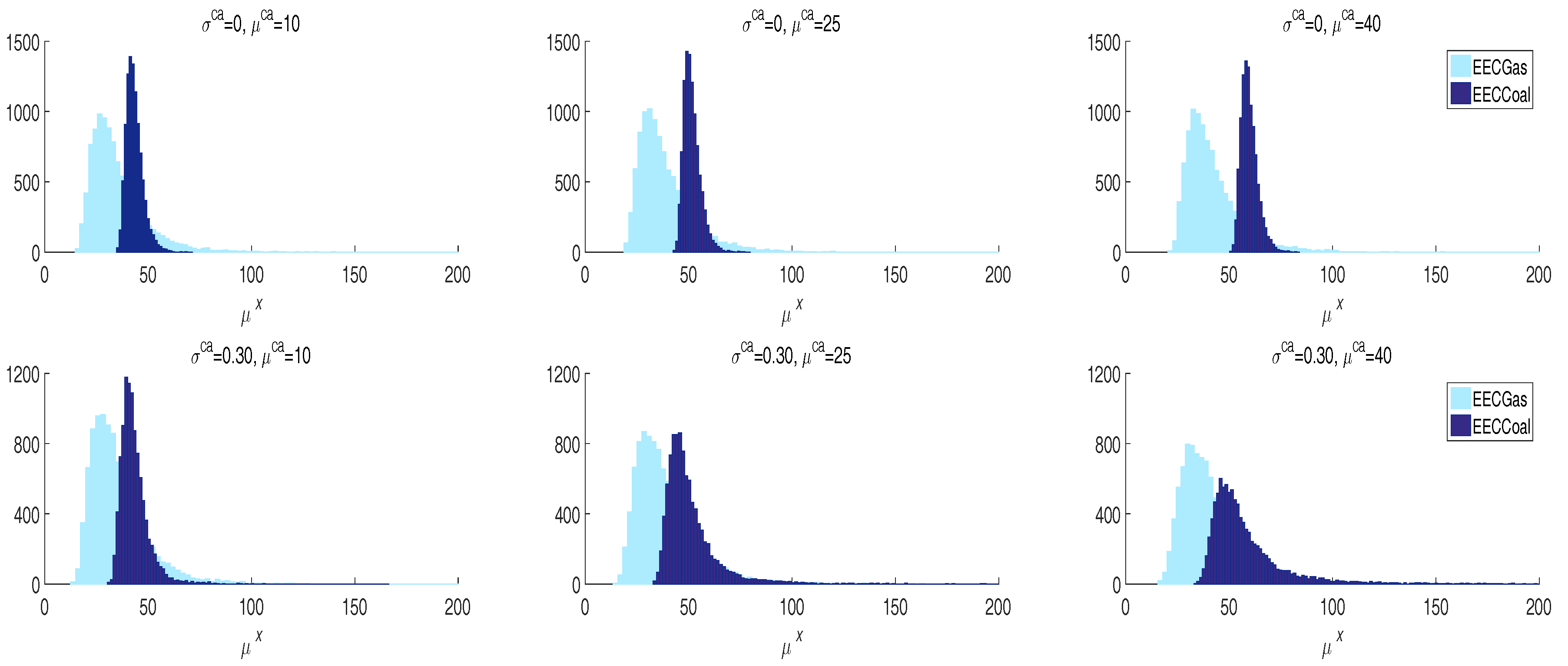
Figure 1 shows sample distributions of gas and coal stochastic EECs in the two carbon volatility scenarios.
Table 2 and
Table 3 report the mean
, the standard deviation (
) and the CVaR deviation (
) of the EEC simulated distributions in each CO
price volatility scenario. The correlation between gas and coal stochastic EEC is also shown.
In the zero CO
volatility scenario, the CO
price level has no effect on the risk of gas and coal stochastic EECs as measured by standard deviation or CVaRD. As shown in
Table 2, the CO
price level affects only the EEC mean (this is a direct consequence of Equation (
A1)).
A very interesting behavior can be observed when CO
prices are assumed to evolve in time according to Equation (
3) with a non-zero volatility. In such a case, within the same CO
volatility scenario, different CO
price levels have different impacts on risk.
Figure 1 shows that as the CO
price level increases, EEC distributions become more asymmetric with long fat tails. The values of both standard deviation and CVaR deviation, reported in
Table 3, increase as the CO
price level increases. Moreover, the CO
price level affects also the correlation between gas and coal stochastic EECs. In fact, the dynamics of CO
price affects the first term in the r.h.s. of Equation (
A1) for both gas and coal sources. As the CO
price level increases, the correlation between gas and coal stochastic EEC increases. As we will show in the following, such features have strong consequences on optimal power system portfolios and on CO
emissions assessment.
3. CO Price Volatility Effects on Optimal Power System Portfolios
In this section, we discuss the effects of integrated environmental and renewable energy policies on optimal power system portfolios.
By integrated environmental and renewable energy policies, we mean energy policies characterized by well-defined renewable penetration targets under well-defined CO
emissions pricing schemes. We will consider two different environmental policy schemes. The first one is a non-volatile ‘carbon tax’ scheme in which the CO
emissions price is fixed (in real terms) for the whole time horizon. The second one is a volatile scheme in which carbon prices are assumed to evolve in time according to Equation (
3) with
. In both scenarios, different CO
price levels (
) are considered. The aim is to quantify the effects of different environmental policies on optimal power system portfolios. The renewable energy policy is defined in terms of a target on renewables’ penetration. In this way, environmental policies will be integrated with renewable energy policies.
By power system portfolio, we mean a generation portfolio matching the yearly load duration curve (and capacity reserve) of a given power system.
Appendix B reviews some basic definitions about power system portfolios, also called systemic portfolios, and provides an analytic characterization of optimal power system portfolios.
We first limit our analysis to generation portfolios with two dispatchable technologies, gas and coal, and one intermittent source, wind. Then, we include a third dispatchable source, nuclear power. In both cases, we determine systemic portfolio frontiers in terms of trade-offs EEC mean-standard deviation
,
and EEC mean-CVaRD
,
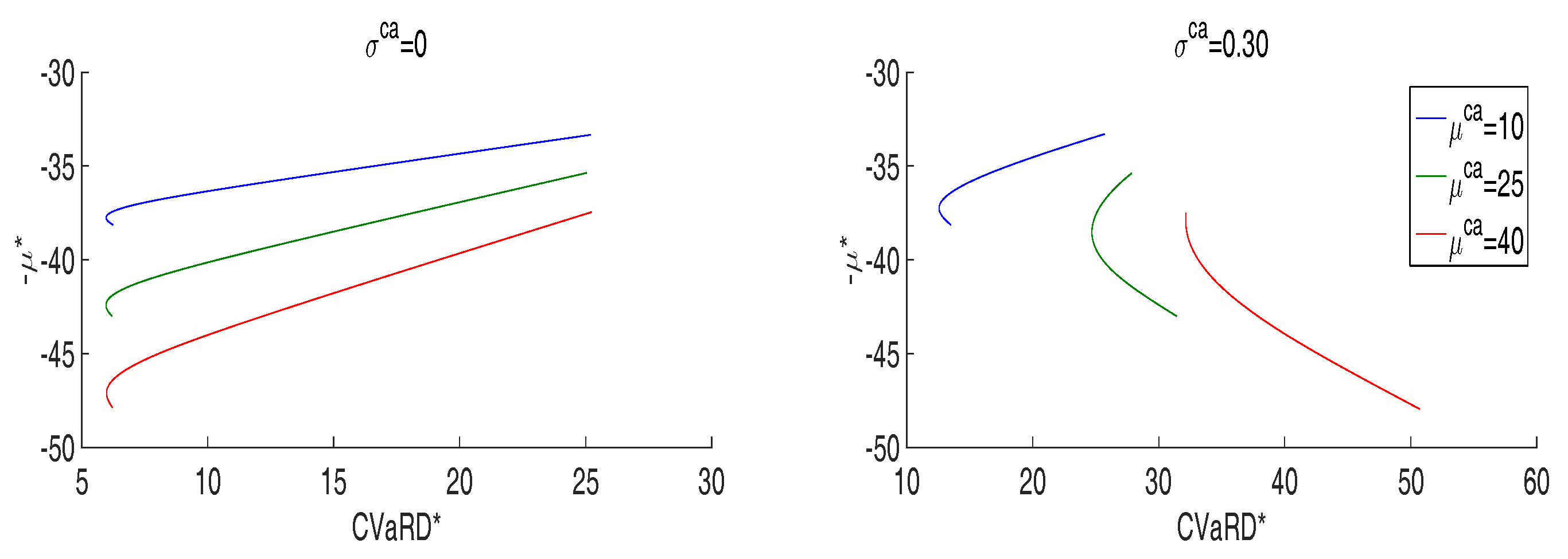
of optimal systemic portfolios (for the CVaRD risk measure, the confidence level has been chosen equal to
). In this way, optimization can be introduced in the stochastic EEC framework, picking up systemic portfolios belonging to the efficient systemic frontier. Risk can be therefore controlled and minimized. A planner could manage risk by selecting the systemic portfolio that minimizes EEC fluctuations around the mean. However, she/he could realize that it might be important to account for extreme events, i.e., EEC values larger than the mean. In this second case, an appropriate risk metric is still a deviation, but an asymmetric one, like CVaRD [
11]. Portfolios with a low CVaRD minimize the risk of ending up with EEC values too much larger than their mean. In this way, CVaRD is able to properly take into account risk from long tails.
3.1. Two Dispatchable Sources and One Intermittent Source: Gas, Coal and Wind
In this research context, CO
price volatility effects on the stochastic EEC of fossil fuels technologies are examined towards illustrating CO
price volatility effects on portfolio selection and on CO
emissions reduction. To this end, the analysis is performed in the cases of
dispatchable technologies, gas and coal, and an
non-dispatchable source, wind with a given penetration
. Using data reported in
Appendix A, we get
$ 2015/MWh. Dispatchable generation technologies are ordered by increasing values of the unitary fixed costs of generation. The coal technology has higher fixed and investment costs with respect to the gas technology. In fact, using data reported in
Table A1 we get:
Gas is therefore Technology 1 and coal is Technology 2.
Systemic portfolios frontiers are determined using Equation (A12) under a two-step procedure. First, for each portfolio composition, i.e., for each vector
, we compute the EEC mean and the risk measure values (standard deviation and CVaRD values) of the optimal systemic portfolio of that subset. Then, the systemic standard deviation frontier is obtained by plotting EEC mean and standard deviation values of optimal systemic portfolios for
and
. In the same way, the systemic CVaRD frontier is obtained by computing EEC mean and CVaRD values of optimal systemic portfolios (the case
is not consider here because it refers to a two-asset, coal and wind, inefficient portfolio).
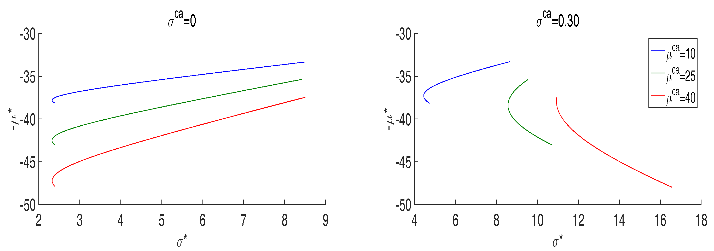
Figure 2 and
Figure 3 display systemic frontiers in the two carbon volatility scenarios
for
. The power system capacity factor is assumed equal to
. The wind penetration has been chosen equal to
, in agreement with the U.S. planned targets as reported in ‘Renewable Electricity Futures Study’ published by the National Renewable Energy Laboratory [
32]. As is well documented in the ‘IEA Wind—2015 Annual Report’ [
33], several European countries have similar targets. The capacity value is assumed equal to
.
Table 4 and
Table 5 report respectively the composition of minimum variance systemic portfolios (mvp) and minimum CVaRD portfolios (mcp) in the two carbon volatility scenarios
for
.
We notice that in each scenario, the composition of the mvp portfolio is very similar to the composition of the mcp portfolio. A variance risk-averse planner and a tail risk-averse planner would select, therefore, very similar power system portfolios.
Table 4 and
Table 5 depict also CO
emission rates of mvp and mcp portfolios. Let us recall that the CO
emissions rate of a generating portfolio is a linear combination of single technology emissions rates, using as weights the fraction of energy generated by each single technology. This means that optimal systemic portfolios are characterized by the emissions rate:
where
and
are respectively the CO
emissions rates (measured in tCO
/MWh) of the gas and the coal technologies. Emissions rates are computed using the values
tCO
/MWh and
tCO
/MWh (see
Table A1).
The efficient systemic frontier, i.e., the locus of system portfolios that have minimum cost among all system portfolios with the same level of risk, is represented in each graph of
Figure 2 and
Figure 3 by the upward sloping part of the curves starting from the minimum variance systemic portfolio in the plane
, or the minimum CVaRD systemic portfolio in the
plane, and ending with the two-asset, gas and wind, systemic portfolio. Efficient systemic portfolios, i.e., systemic portfolios belonging to the efficient frontier, show well-defined cost-risk and CO
emissions-risk trade-offs. In the specific, minimum variance portfolios, as well as minimum CVaRD portfolios are characterized by the maximum CO
emission rate. In fact, among efficient systemic portfolios, minimum risk portfolios (mvp and mcp portfolios) are characterized by the maximum coal component. Moving from left to right, efficient systemic portfolios display increasing risk, as measured by the standard deviation or CVaRD, decreasing EEC means and decreasing CO
emissions rates. This is due to the fact that the gas component
increases (and the coal component
reduces) as we move from left to right along the efficient systemic frontier to end up with
(
), the value that defines the optimal gas and wind system portfolio.
In the zero CO
price volatility scenario (i.e., under a deterministic carbon tax), the CO
price level has no effect on risk of efficient system portfolios. Since, the composition of minimum risk portfolios is not affected by the CO
price level, the efficient systemic portfolio frontier is invariant, i.e., it is composed of portfolios with the same mixes of gas, coal and wind and the same CO
emission rates. As shown in
Figure 2 and
Figure 3, the only effect is an increase of the EEC mean, and as
increases, the efficient frontier moves south.
Under the volatile CO scenario, two main effects are to be pointed out.
The first effect can be observed by comparing among them efficient frontiers within the same CO
volatile scenario for different values of the CO
price level (see
Figure 2 and
Figure 3, left panels). Differently from the zero CO
price volatility scenario,
Table 4 and
Table 5 show that the mvp and the mcp portfolios compositions are influenced by the CO
price level. As the CO
price level increases, the gas component of both, mvp and mcp portfolios, increases, and this fact leads to a reduction of the CO
emission rate and to an increase of the risk. Under the volatile CO
pricing scheme, efficient systemic frontiers alter because, as the CO
price level increases, the most emitting systemic portfolios become inefficient. In this sense, the joint effect of CO
price level and CO
price volatility reduces CO
emissions and increases risk in the power sector.
The second effect can be observed by comparing efficient frontiers in the two volatility scenarios under the same CO
price level.
Table 4 and
Table 5 show that the composition of the mvp and the mcp portfolios is influenced by the CO
price volatility. In the volatile scenario, the gas component of such optimal portfolios is greater with respect to the gas component in the non-volatile carbon tax scenario. This fact leads to a reduction of both expected cost and CO
emission rate, as well as to an increase of the risk. The efficient systemic frontiers alter because the CO
price volatility makes the most emitting systemic portfolios inefficient.
Finally, we notice from Equation (A12) that the capacity value does not affect the risk of the systemic frontier portfolios, but it influences only EEC mean values.
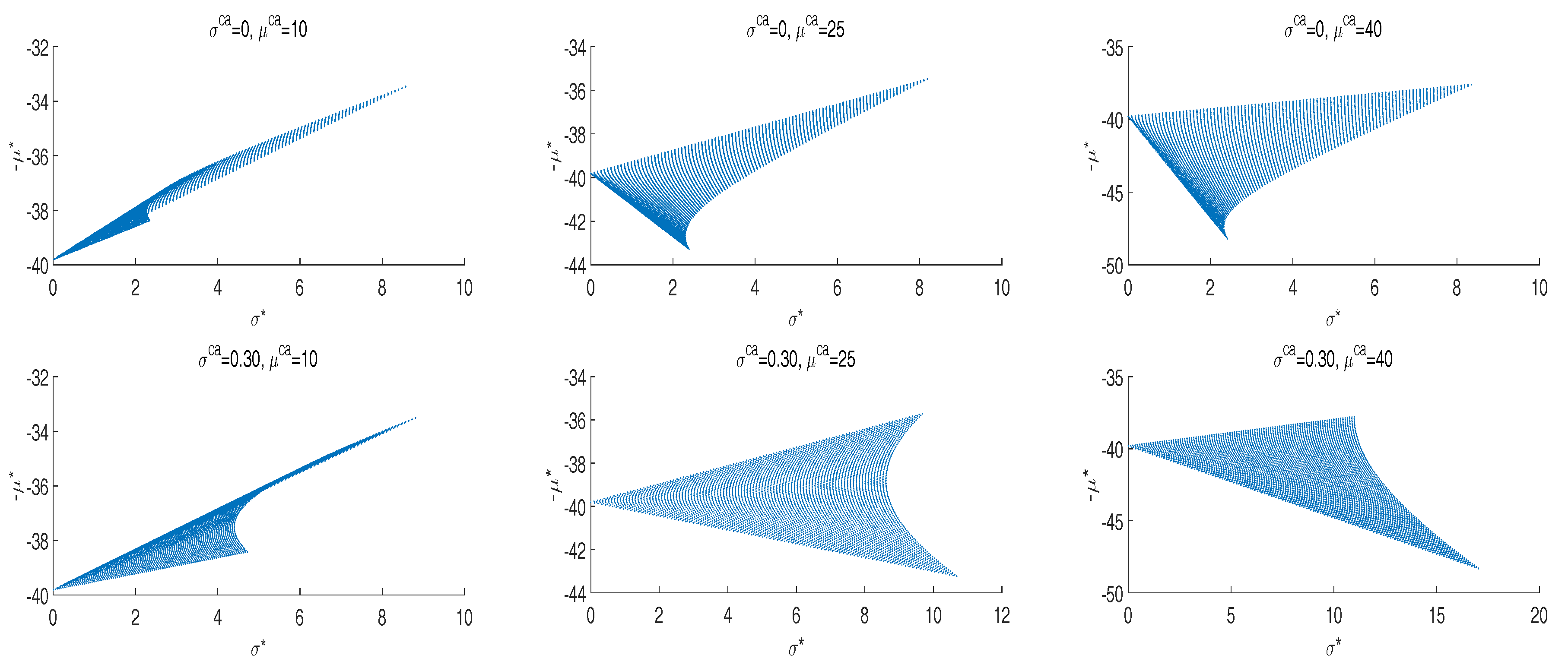
3.2. Three Dispatchable Sources and One Intermittent Source: Gas, Coal, Nuclear Power and Wind
We now discuss the effects of CO
price volatility on portfolio selection and CO
emissions assessment in the case of
dispatchable technologies, gas, coal and nuclear power, and an
non-dispatchable source, wind, with a given penetration
. We will see that when a carbon-free dispatchable source, like nuclear power, is included in the analysis, the CO
price volatility has a different impact on efficient systemic portfolio frontiers. As in the previous subsection, systemic portfolio frontiers will be determined using Equation (A12) in which generation assets are ordered in this way: gas is Technology 1; coal is Technology 2; and nuclear is Technology 3. Coal and nuclear technologies have higher fixed and investment costs with respect to the gas technology. Using data reported in
Table A1, we get, in fact,
Moreover, under our hypothesis of three sources of risk, namely fossil fuel prices and CO
prices, the nuclear EEC is a deterministic quantity because the electricity production from the nuclear source does not burn fossil fuels and does not release CO
. The nuclear asset can be seen as a risk-free asset in an otherwise risky portfolio, and its contribution to risk reduction by diversification can be relevant [
11,
30]. Using data reported in
Appendix A, we get
$ 2015/MWh.
Systemic portfolio frontiers are determined using the same two-step procedure discussed in the previous subsection. However, if we compute EEC mean and standard deviation values, as well as EEC mean and CVaRD values of optimal systemic portfolios, in this four-asset case, such values generate a two-dimensional region in the plane
and in the plane
, respectively (see
Figure 4 and
Figure 5). We call this two-dimensional region the ‘optimal systemic set’. The efficient systemic frontier will be then determined by selecting optimal systemic portfolios that for each level of risk have minimum cost. This is represented by the upper border of the optimal systemic set, starting in each panel of
Figure 4 and
Figure 5 from the vertical axis and ending with the two asset, gas and wind, optimal systemic portfolio.
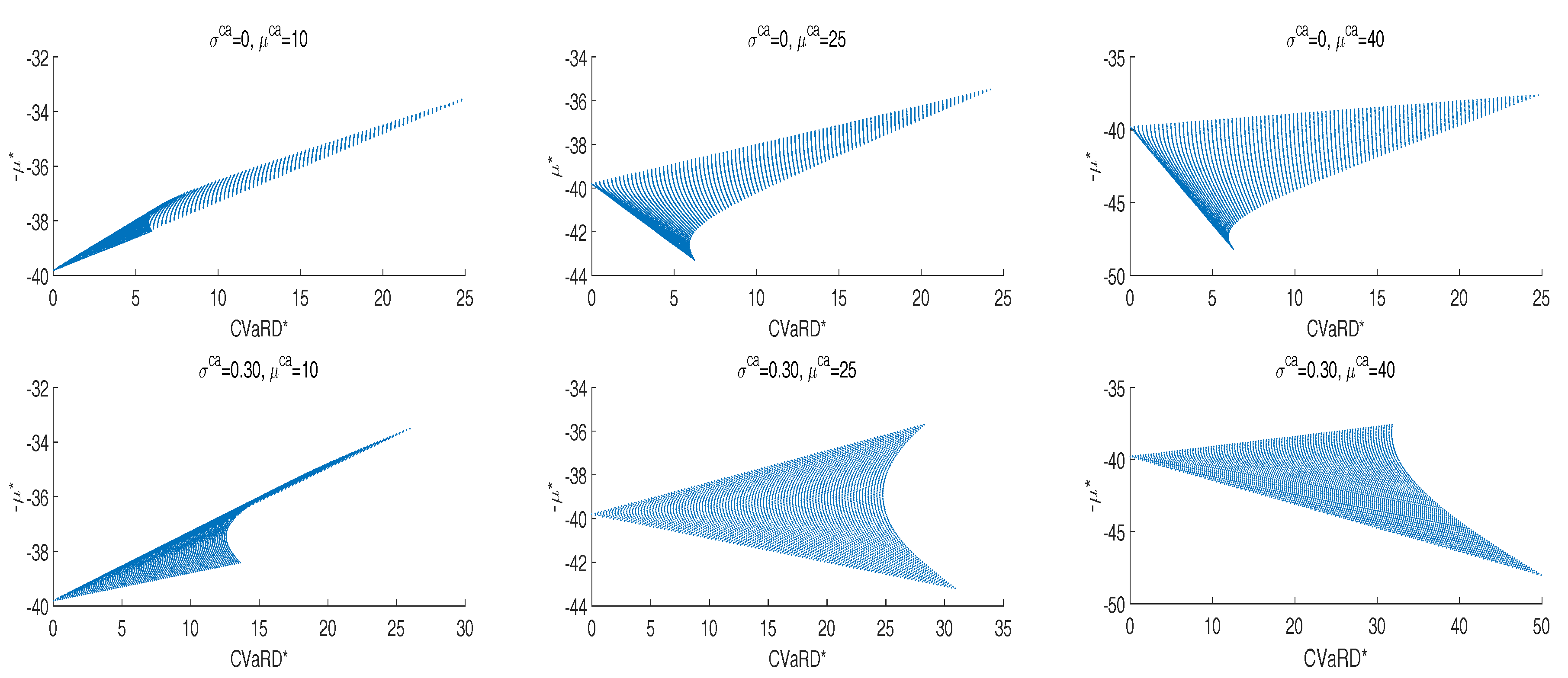
Figure 4 displays optimal systemic sets in the plane
for the two carbon volatility scenarios
and
. As in the previous subsection, the wind penetration has been chosen equal to
and the capacity value equal to
. The power system capacity factor is assumed equal to
. The optimal systemic set is depicted for values
of the gas portfolio component (the case
is characterized by three asset, coal, nuclear and wind, inefficient systemic portfolios, with the exception of the subset
which consists of an efficient two-asset, nuclear and wind, risk-free systemic portfolio; this case is not discussed in the empirical analysis).
In both volatility scenarios, with the exception of the lowest CO
price level case
, systemic efficient frontiers are straight lines. In the presence of a risk-free dispatchable asset with unlimited availability, this is a general result due to the mathematical properties of the so-called risk ‘deviation measures’ [
20,
34] (in our analysis, the standard deviation and the CVaR deviation). In such cases, efficient systemic portfolios are composed by mixtures of gas, nuclear power and wind. Coal is excluded by the portfolio composition because of its high generation cost for
and
. For
, the picture is very different. In this case, we can identify an efficient systemic portfolio, which is tangent to the three-asset, gas, coal and wind efficient systemic frontier. The composition of such a portfolio is
in the case
and
for
. The four-asset efficient systemic frontier is then a straight line until the tangent portfolio is reached. Then, at the right of the tangency point, the systemic frontier coincides with the three-asset, gas, coal and wind, efficient systemic frontier (nuclear power is excluded). In the straight line part of the efficient frontier, efficient systemic portfolios are composed by mixtures of the tangent generation portfolio, the nuclear and wind assets.
The same representation holds also when tail risk, measured by CVaR deviation, is taken into account.
Figure 5 displays systemic efficient frontiers in the plane
.
As in the standard deviation case, systemic efficient frontiers are straight lines in both CO
price volatility scenarios for
and
. Efficient systemic portfolios are composed by mixtures of gas, nuclear power and wind (coal is excluded). In the case
, a tangent portfolio can be identified also under the CVaRD risk measure in both CO
price volatility scenarios. The composition of such a portfolio is
in the case
and
for
. When tail risk is taken into account through the CVaRD measure, the coal component of both tangent portfolios is larger than the coal component of tangent portfolios computed under the standard deviation risk measure. The reason is that for
, the tail of the gas EEC distribution is more pronounced with respect to the tail of the coal EEC distribution in both CO
volatility scenarios (see
Figure 1).
Efficient systemic portfolios show a well-defined cost-risk trade-off in both CO
price volatility scenarios. As depicted in
Figure 4 and
Figure 5, moving along the efficient systemic frontier from left to right, the risk increases and the expected generation cost decreases. Yet, a more complicated relationship exists between CO
emission rate and risk. In fact, when a tangent systemic portfolio exists (in our case, for the lowest CO
price level
), moving along the efficient frontier from left to right (i.e., going towards increasing risk and decreasing cost), the CO
emission rate of efficient systemic portfolios linearly increases until the tangent portfolio is reached, then it progressively decreases until reaching the two-asset, gas and wind, systemic portfolio. In the remaining cases (
and
), moving along the efficient frontier from left to right, both the CO
emission rate and the risk of efficient systemic portfolios monotonically increase until the efficient gas and wind systemic portfolio is reached.
We must notice that when the nuclear asset is included in the analysis, systemic frontiers are very sensitive to the CO
price level also in the zero volatility scenario. As shown in
Figure 4 and
Figure 5, the CO
price level influences the composition of efficient systemic portfolios in both the non-volatile and the volatile scenarios, by excluding coal in the composition of efficient systemic portfolios for
and
. Moreover, in the non-volatile scenario, the CO
price level influences the CO
emission rate of efficient systemic portfolios without affecting risk. This is an important difference with respect to three-asset, gas, coal and wind, case.
4. Concluding Remarks
The analysis developed in this paper offers to policy makers a global view of the power system useful for assessing integrated environmental and renewable energy policies. It allows a policy maker to value the impact of CO price volatility on CO emissions reduction and on the overall risk of efficient systemic portfolios, also comparing the effects produced by market-based mechanisms for CO pricing with those produced by non-volatile carbon tax schemes.
Our results indicate that in some power system configurations, the CO price volatility can play a crucial role in the CO emissions reduction process, because it forces one to reduce in an efficient way the coal component of generation portfolios for risk-aversion reasons. This happens when the (non-renewable) dispatchable part of the power system portfolio is fully composed of fossil fuel, gas and coal technologies. In this case, we demonstrated that under volatile CO price scenarios, the CO price level has a larger and more substantial impact on CO emissions reduction with respect to the impact it has in a non-volatile scenario. In particular, under volatile CO prices, increasing CO price levels leads to reduction of the CO emission rate and to an increase of the risk of efficient systemic portfolios. In such power systems, we cannot reduce CO emissions without increasing risk. Policy makers must be aware that setting, for example, a suitable target on the CO emission rate, they determine in a unique way the generation cost and the risk level in the power system. Alternatively, policy makers can set a target on the generating cost of electricity, thus uniquely determining the risk and the CO emission rate of the power system.
When a carbon-free dispatchable asset, like nuclear power, is included in the analysis, the picture is very different. The CO
price level has an important impact on CO
emissions also in the zero volatility scenario. In such a case, the CO
emission rate of efficient systemic portfolios can be reduced without affecting risk. These are important indications for an energy planner concerned with environmental issues and economic issues [
35].
Energy planners have to pay great attention when they project CO pricing mechanisms. Depending on the power sources’ composition, the same CO pricing mechanism may produce very different effects. As has been shown in the paper, a non-volatile carbon tax scheme for pricing CO emissions can produce significant effects on the power system in the presence of a carbon-free dispatchable source, like nuclear power, but it may have negligible effects if the dispatchable part of the power system portfolio is fully composed by fossil fuel, gas and coal, sources. On the other side, market-oriented mechanisms for CO pricing, introducing CO price volatility, can produce relevant effects on CO emissions and on the overall risk of efficient systemic portfolios in both power system configurations.
As governments are the planner subjects for energy choices, they have the duty to promote coherent externality pricing mechanisms and technologies that allow reaching environmental and renewable energy policy targets, providing clear signals to direct private investments [
36]. From this point of view, the most important and difficult task is to find appropriate instruments and strategies for inducing rational investors to modify their generation portfolios according to suitable environmental and renewable energy policies. From this point view, our approach can give a quantitative support for directing and giving assessments for public actions and interventions aiming at reconciling market logics with societal benefits.
Although the empirical analysis is performed on U.S. data, most of the obtained results can be extended to other countries all around the world. In fact, the costs of generating technologies observed in many OECD countries share relevant analogies with cost data provided by the U.S. Department of Energy [
37]. If CO
costs are included in the analysis, the gas technology may be the lowest cost option not only in the United States, but in many other countries.
We remark that the results obtained in the empirical analysis are country specific and cannot be necessarily fitted to all countries throughout the world. However, the proposed methodology is general and can be used to perform similar analyses for different countries involving their own generation technologies’ cost structures, challenging energy targets, technological advances and political, economic, social and managerial issues. For example, it can be applied in the case in which the coal technology is the lowest cost option, as may happen in those countries characterized by very low coal generation costs such as Germany, China and Korea. It can be applied also in the case in which nuclear is the lowest cost option, e.g., as in France, Japan, China and Korea.
Furthermore, we must point out that the dynamics of fossil fuel prices is also country specific. For example, the dynamics of fossil fuel prices observed in EU countries is very different from the dynamics observed in the USA. Roques et al. [
10] put in evidence that the correlation between log-returns of coal and gas market prices is very high. Although in recent years, gas and coal prices showed a significant decoupling, it would be interesting to investigate the effects of fossil fuels’ cross-correlation on portfolio selection and CO
emissions assessment. The proposed pricing model can be extended to account for correlation, mean reversion [
11] and other dynamical features.
These important topics will be left to future investigations.


