Article

A Bottom-Up Model for Household Load Profile Based on the Consumption Behavior of Residents

School of Electrical Engineering, Southeast University, Nanjing 210096, China
*
Author to whom correspondence should be addressed.
Energies 2018, 11(8), 2112; https://doi.org/10.3390/en11082112
Submission received: 20 June 2018 / Revised: 3 August 2018 / Accepted: 13 August 2018 / Published: 14 August 2018
(This article belongs to the Section F: Electrical Engineering)

Abstract

:
The forecasting of the load profile of the domestic sector is an area of increased concern for the power grid as it appears in many applications, such as grid operations, demand side management, energy trading, and so forth. Accordingly, a bottom-up forecasting framework is presented in this paper based upon bottom level data about the electricity consumption of household appliances. In the proposed framework, a load profile for group households is obtained with a similar day extraction module, household behavior analysis module, and household behavior prediction module. Concretely, similar day extraction module is the core of the prediction and is employed to extract similar historical days by considering the external environmental and household internal influence factors on energy consumption. The household behavior analysis module is used to analyse and formulate the consumption behavior probability of appliances according to the statistical characteristics of appliances’ switch state in historical similar days. Based on the former two modules, household behavior prediction module is responsible for the load profile of group households. Finally, a case study based on the measured data in a practical residential community is performed to illustrate the feasibility and effectiveness of the proposed bottom-up household load forecasting approach.

1. Introduction

Electrical load forecasting is a significant activity in the power grid and is involved in many applications, such as energy dispatching for generation, energy management for demand, and energy trading for the electrical market [1,2,3]. Load forecasting generally contains the predictions for household, commercial, and industrial load, in which the household load profile is hard to predict due to the complexity and diversity of household energy consumption. Moreover, with the development of economy and living standards, energy consumption in the household sector has contributed to an increasing proportion of aggregate energy consumption (e.g., about 12% in China, 27% in European, 36% in American). Therefore, it is necessary and meaningful to study the modelling method of the household load profile with high prediction accuracy [4].
Currently, there are two common approaches for the modelling of the load profile: one is the bottom-up method, and the other is the statistical method. In the bottom-up method, the terminal appliance is the study object and the focus is on the consumption model formulation of each terminal appliance [5,6]; while in the statistical method, the study object is to describe the characteristics of the input data based on a set of measured load profiles, and then a prediction model is formulated according to the extracted character [7,8]. Obviously, although the bottom-up method requires a large amount of data that can reflect the consumption behavior of household appliances, it has a high prediction accuracy. However, the difficulty of data acquisition has limited further development of the bottom-up method in the past. However, in recent years, the increased deployment of smart infrastructure in households has created new prospects for electricity load forecasting, especially for the bottom-up prediction method [9]. For example, smart sockets can collect and upload energy consumption information about each appliance to the data center with WiFi communication which will contribute to the efficiency and accuracy of household load forecasting.
In the literature, the abovementioned modeling methods have been studied extensively. In regard to the statistical modelling method, the authors in reference [10] proposed a multiple linear regression model to forecast the total electricity consumption and maximal demand considering social-economic factors like the dwelling type, number of bedrooms, and household composition. Wang et al. [11] put forward a decomposition approach to model the electricity demand trend by dividing historical time series into a number of components based on the seasonality and day of week. In reference [12], the authors designed a time varying multiple regression model for hourly electricity load forecasting considering the changes in customer behavior and utility production efficiency. Stephen et al. [13] presented a framework for analyzing the consumption habits of domestic energy customers assuming that electric loads obey a non-stationary multivariate Gaussian distribution. The authors in [14] proposed a functional vector autoregressive state space model to forecast the future electricity demand, aiming to apply it at some aggregation level between regional and nation-wide grids. For the bottom-up modelling method, Capasso et al. [15] proposed a bottom-up model to establish the load profile of a residential area by aggregating the consumption of individual appliances. Reference [16] presented a high-resolution model of household electricity consumption based upon a combination of measured and statistical data which uses the 1-min cycle power use characteristics of a single appliance as the main building block. The authors of reference [17] proposed a stochastic bottom-up model to forecast domestic lighting demand by using three state non-homogeneous Markov chains to describe the occupancy patterns of lighting demand. Moreover, Paatero et al. [18] modeled the starting of individual appliances as random processes, depending on seasonal and social factors. The authors of reference [19] designed a forecasting model to investigate the effects of occupant behavior, appliance stock, and efficiency on the electric load profile of an individual household. Based on the work in reference [19], the stochastic bottom-up approach for electric loads was extended to cover domestic hot water and space heating demands due to the high proportion of heat demand in the German residential sector [20]. The authors of reference [21] introduced big data mining technology into the behavioral analysis of energy consumption, and then performed extensive experiments using real-world context-rich smart meter datasets. In reference [22], the authors presented a high-resolution model of domestic energy consumption for individual domestic dwelling based on occupant activity and appliance use.
The above research shows that a large variety appliances exists in households and their use is greatly influenced by living habits, family structure, and the environment. This also means that household consumption behavior can reflect the influencing degree of the abovementioned factors. However, in the current research on the bottom-up modelling method, few studies have taken the extraction process of historical days into consideration. It is obvious that there are numerous historical days in which some days differ from the forecasted day in terms of weather condition or weekday type. If historical days without a high degree of similarity are used to predict the profile, then the prediction accuracy will be decreased dramatically. Therefore, this paper focuses on the formulation of a bottom-up model for the household load profile based on the analysis of consumption behavior for each appliance. In order to extract the consumption behavior precisely from historical data, a similar day extraction process is proposed which considers the factors that significantly influence the energy consumption. Such extraction processes can choose similar historical days based on the similarity degree with the forecasted day and reduce the influence of non-similar days on the predicted profile. In brief, the main contributions of this paper are as follows:
  • A forecasting framework is proposed for the household load profile with the bottom-up modelling method considering the consumption behavior of residents.
  • A similar day extraction model is formulated to choose similar days by comparing external environmental factors and household internal influence factors on the energy consumption in order to enhance the prediction accuracy of residents’ consumption behavior.
  • A case study is conducted based on the measured data in a residential community containing 64 households. Furthermore, load profiles of families in different categories (i.e., worker family, senior family, and senior + worker family) are forecasted separately to verify the effectiveness of proposed approach in different family categories.
An electricity forecasting framework is introduced in Section 2. Section 3 mainly introduces the data acquisition and processing. In Section 4, group household consumption behavior is modeled. Then, a case study is presented in Section 5. Finally, the paper is concluded in Section 6.

2. Electricity Forecasting Framework

Residents’ electricity consumption is consistent with the consumption of many single households, while the consumption of a single household is consistent with the consumption of all household appliances. Based on this, an electricity forecasting framework is proposed by the bottom-up modeling method. The consumption behavior of each household appliance is firstly analyzed and modeled by extracting the consumption characteristics of the corresponding appliance in similar historical days. Then, the forecasting model of group household electricity consumption is formulated by accumulating the consumption of all appliances in all households.
For a single household, energy consumption is often determined by the residents’ living habits, but their behavior is accompanied by a certain degree of randomness due to various factors, including external environmental factors and family internal factors [23]. External environmental factors mainly concern the weather conditions, types of weekdays, emergencies, etc., and family internal factors mainly contain family members’ types, income statuses, and so on. Generally, similar factors will have similar effects on the consumption of household appliances. Therefore, it is feasible to model household consumption behavior with the statistical characteristics of appliance consumption in similar historical days. Accordingly, a forecasting framework of group household consumption is proposed based on historical similar day selection and probability statistics, as shown in Figure 1. The similar day extraction module is used to evaluate the influence of external environmental factors and family internal factors on the electricity consumption of residents. A household behavior analysis module is used to analyze the switch states of household appliances in the past, reflecting the residents’ decisions about the behavior of appliances. The household behavior prediction module is responsible for the prediction of group households in the forecasting day.

3. Data Acquisition and Processing

3.1. Data Acquisition

In order to forecast the load profile, the consumption data of household appliances needs to be collected with an intellectual socket which measures consumption powerand communicates with the data center. During the period of data collection, each appliance in the household has to be connected with an intellectual socket. No matter whether a household appliance is under operation or not, the socket will send the power consumption information to the data center at each recording point with WiFi communication technology.

3.2. Data Processing

In the process of actual data recording, transmission and storage, deviation in accuracy and continuity of data may occur due to various disturbances. Therefore, it is necessary to rehandle the collected data. Assume that there are N historical days and each day has J recording points. If it is assumed that D j , n is the load data at recording point j on the nth day, α max j , n is the maximum value of the load variation ratio between point j and j 1 in the n 1 days. The horizontal comparison method of data can be expressed by the following formula:
D ( j , n ) D ( j 1 , n ) D ( j 1 , n ) > α max ( j , n ) α max ( j , n ) = max D ( j , n d ) D ( j 1 , n d ) D ( j 1 , n d ) d = 1 , 2 , , n 1 ; j = 1 , 2 , , J ; n = 1 , 2 , , N ,
where d represents the interval days including the current day. When D ( j , n ) satisfies the above conditions, D ( j , n ) is bad data. Hence, D ( j , n ) needs to be modified with following formula:
D ( j , n ) = μ 1 D ( j , n 1 ) + μ 2 D ( j , n 2 ) + + μ n 1 D ( j , 1 ) ,
where μ 1 , μ 2 , , μ n 1 are the corresponding weights.
In order to analyse the consumption behavior for household appliances, the switch state of each appliance has to be counted for historical days. Household appliances generally have three states: the off state, operation state, and standby state. Since the standby state of an appliance has low energy consumption, the standby state can be considered to be the off state [24]. Based on the data of each appliance’s consumption power, switch state of each appliance can be obtained with following formula:
S j i = 1 D j i > P s i 0 D j i P s i
where S j i represents the switch state of appliance i at recording point j, D j i represents appliance i’s consumption power at point j, and P s i is the consumption power of appliance i in the standby state. When data D j i is greater than the standby power, it demonstrates that appliance i is on operation state, while when D j i is less than or equal to P s i , it demonstrates that appliance i is in the off state.

4. Bottom-Up Forecasting Model for Group Household

According to the framework in Figure 1, the concrete process for the group households’ load profile is as given below, including a similar day extraction module, household behavior analysis module, and household behavior prediction module.

4.1. Similar Day Extraction Module

It is clearly that the load profile is predicted based on the consumption data in the historical days. However, there are numerous historical days, and different days will have different degrees of similarity with the forecasting day. Consequently, the choice of days selected among the historical days is very important for the prediction accuracy of the load profile. Generally, employing historical days with the greatest degree of similarity will contribute the promotion of prediction accuracy. Therefore, it is necessary to select similar historical days. The similar day extraction module can be implemented by three modules: the historical data preprocessing module, the similarity feature vector computing module, and the similarity factor sorting module.

4.1.1. Similarity Feature Vector Computing Module

Household consumption behavior is affected by external environmental factors and household internal factors. Therefore, in the selection of similar historical days, environmental factors and household factors must be both considered. Consequently, a similarity feature vector is used to measure the similarity degree, as follows:
X = α δ λ θ ε ,
where, X is the similarity feature vector; α is the human comfort index factor; δ is the time gap factor; λ is the weekday type factor; θ is the major event factor; and ε is the family category index.
(1)
Human comfort factor
In order to quantitatively measure the influence of environmental factors (e.g., ambient temperature, relative humidity, and wind speed) on the electricity consumption of households, the human comfort index ( α ) is used to measure the degree of similarity between the forecasting date and the historical date in the weather. The formula is as follows [25]:
α = 1.8 T a 0.55 ( 1.8 T a 26 ) ( 1 R H ) + 9.2 ( 9 + 10.9 u u ) + 32 ,
where, T a is the ambient temperature; R H is the relative air humidity; and u is the average wind speed.
(2)
Time gap factor
From a long-term perspective, since residents’ load tends to increase periodically over time, the long-term regularity of residents’ consumption behavior needs to be measured by the time gap ( δ ) which indicates a degree of similarity between the forecasting date and the historical date in the long-term time span. Based on the principle that the time gap is increased while the degree of similarity is weakened, the time gap can be formulated as
δ h ( d ) = β 1 d β 2 int ( d / y e a r ) ,
where, d is the number of days from the prediction day to the historical day; β 1 and β 2 are attenuation coefficients, generally ranging from 0.9 to 0.98; y e a r is the constant with y e a r = 365 .
(3)
Weekday type factor
From a short-term point of view, household consumption behavior within a week also shows a certain degree of repetitiveness and regularity. For example, the load profile of office workers will be quite different between workdays and weekends, but will have a certain similarity in the workdays in different weeks. Therefore, this paper uses the week type factor ( λ ) to measure the degree of similarity on weekday types between the forecasting day and the historical day. The formula is as follows:
λ p = 1 f ( w p ) f ( w h )
f ( w p ) , f ( w h ) = 0 . 1 , p , h = 1 0 . 2 , p , h = 2 , 3 , 4 0 . 3 , p , h = 5 0 . 7 , p , h = 6 1 , p , h = 7 ,
where w p is week type of forecasting day; w h are week types of historical days; p and h take 1, 2, 3, 4, 5, 6 and 7 from Monday to Sunday; and f ( w p ) and f ( w h ) are the mapping values of w p and w h , respectively.
(4)
Major event factor
Due to the impact of some major events, such as holidays, serious natural disasters, etc., residents’ electricity consumption behavior will fluctuate in a short period of time. Therefore, it must be included in the similarity feature vector to measure the influence on household consumption behavior. The formula is defined as follows:
θ = 1 , d p = d h 0 , d p d h d h 0 , 1 , d p 0 , 1
where θ = 1 if the historical day ( d h ) and forecasting day ( d p ) are the same major event, otherwise θ = 0 ; different major event types are represented by different values between (0, 1).
(5)
Family category index
Family in different categories will have different levels of energy consumption due to differences in living habits. The typical family categories can be broadly divided into four parts: worker family, senior family, senior + worker family, and vacant house. The family category index values ( ε 0 , 1 ) can be assumed to be 0.25, 0.5, 0.75, and 1 for the above four categories, respectively. The family category index is closely connected with the household members and their daily schedules. That is, if the household members and the daily schedule remain relatively fixed over a period of time, then the index ε remains constant. Otherwise, the index ε has to make a corresponding change according to the current family category.

4.1.2. Similarity Factor Sorting Module

The degree of similarity of feature vectors between the forecasting day and historical day can be measured by the Euclidean distance. However, there is a large difference in the magnitudes of the factors’ values, and some factors with large values will weaken the influence of factors with small values in the comparison of similarity feature vectors. Therefore, in order to solve the problem and improve the accuracy of the selection of historical similar days, it is necessary to normalize the factors in the similarity feature vector.
α * = α / max ( α ) δ * = δ / max ( δ ) λ * = λ / max ( λ ) θ * = θ / max ( θ ) ε * = ε / max ( ε ) ,
where, α , δ , λ , θ , and ε are factor vectors that consist of the factors in historical days and the forecasting day; and α * , δ * , λ * , θ * , and ε * are normalized factor vectors. After normalization, the similarity feature vector (X) can be reformed as a normalized similarity feature vector ( X * ). The Euclidean distance is calculated as follows [26,27]:
l ( X p * , X h * ) = α p * α h * 2 + δ p * δ h * 2 + λ p * λ h * 2 + θ p * θ h * 2 + + ε p * ε h * 2 ,
where, X p * = α p * δ p * λ p * θ p * ε p * and X h * = α h * δ h * λ h * θ h * ε h * are feature vectors of the forecasting day and historical day, respectively. Since the Euclidean distance measures the degree of dissimilarity between two similarity feature vectors, the similarity between two feature vectors is opposite to the Euclidean distance. Accordingly, the similarity degree can be expressed by following formula:
s ( X p * , X h * ) = 1 1 + l ( X p * , X h * ) .
Since there are total of N historical days in the prediction, we can obtain a similarity degree set, s = [ s 1 , s 2 , , s N ] . Consequently, M historical days with the highest similarity degree can be selected by following formula:
h 1 = max s = max ( s 1 , s 2 , , s N ) h 2 = max ( s \ h 1 ) = max [ ( s 1 , s 2 , , s N ) \ h 1 ] h M = max ( s \ h M 1 ) = max [ ( s 1 , s 2 , , s N ) \ ( h 1 , h 2 , , h M 1 ) ] ,
where, h M = h 1 , h 2 , , h M denotes the set of historical similar days in descending order by similarity degree; s \ h M 1 denotes the remaining historical days except the M 1 days with the highest similarity degree.

4.2. Load Profile for Group Household

4.2.1. Household Behavior Analysis Module

In this section, a bottom-up modeling method is used to find the electricity consumption behavior model based on the behavioral probabilities of each household appliance in similar historical days. For M similar days in a single household, the historical behavior probability ( p h j i ) of home appliance i being used at recording point j is calculated as the following formula:
p h j i = m = 1 M S m j i M ,
where S m j i = 1 represents home appliance i being under operation at recording point j on a similar day (m), and S m j i = 0 represents that home appliance i is in the off state. p h j i shows the probability of appliance i being operated at recording point j on the historical day. Therefore, the historical behavior probability ( p h i ) of appliance i at all recording points can be obtained with
p h i = { p h 1 i , p h 2 i , , p h j i , , p h J i } .
Consequently, the historical electricity consumption behavior model of all household appliances can be expressed with p h , as shown in the following formula:
p h = { p h 1 , p h 2 , , p h i , , p h I } ,
where I is the number of household appliances.

4.2.2. Household Behavior Prediction Module

Based on the historical behavior probability and consumption power of a household appliance, the consumption model of a single appliance shown by
P i ( j ) = p h j i P o i ,
where P i ( j ) is the expected power consumed by household appliance i at recording point j; and P o i is the consumption power of household appliance i. Since the historical behavior probability of an appliance is calculated from the historical days with the highest degree of similarity, the behavior probability can be considered to be the operation probability of the corresponding appliance on the forecasting day. Consequently, Equation (17) can be considered to be the forecasting result of appliance i at recording point j. Furthermore, the load profile of a single household can be predicted by accumulating the energy consumption of all I appliances in the family. That is
P c ( j ) = i = 1 I P i ( j ) = i = 1 I p h j i P o i ,
where, P c ( j ) is the expected power of electricity consumption in household c at recording point j. As for the load profile of group households, we can accumulate the whole energy consumption of all group households. If it is assumed that there are C households in the group, the group load can be expressed as
P g r o u p j = c = 1 C P c ( j ) .

5. Case Study

In this section, a residential community containing 64 households is taken as an example to show the effectiveness of the proposed electricity forecasting framework. In the community, 64 households have four kinds of home appliances: lighting appliances, resistance appliances (e.g., electric water heater, rice cooker), motor appliances (e.g., refrigerator, air conditioner, rangehood), and power electronic appliances (e.g., television, computer). Each household was equipped with an intellectual socket to collect the energy consumption of household appliances, and the sampling interval of the smart sockets was 10 min. Historical data was collected from 1 July 2017 to 31 July 2017, and the load profile of 31 July 2017 was predicted with the proposed approach. Additionally, basic information was collected everyday, including environmental data, events, weekday type and date, which is shown in Table A1.

5.1. Forecasting Result for a Single Household

One household in the community was selected for the prediction of energy consumption for 31 July 2017 with the historical data. The partial household appliances in this family are shown in Table 1. Based on the collected data, the degree of similarity among the historical days and forecasting day in July is shown in Figure 2. From the figure, one can see that the 5 days with the highest similarity degree were 27 July with 0.86658, 25 July with 0.86534, 26 July with 0.82582, 24 July with 0.82448, and 20 July with 0.81342. According to the 5 extracted similar days, the energy consumption of this single household for July 31 was predicted.
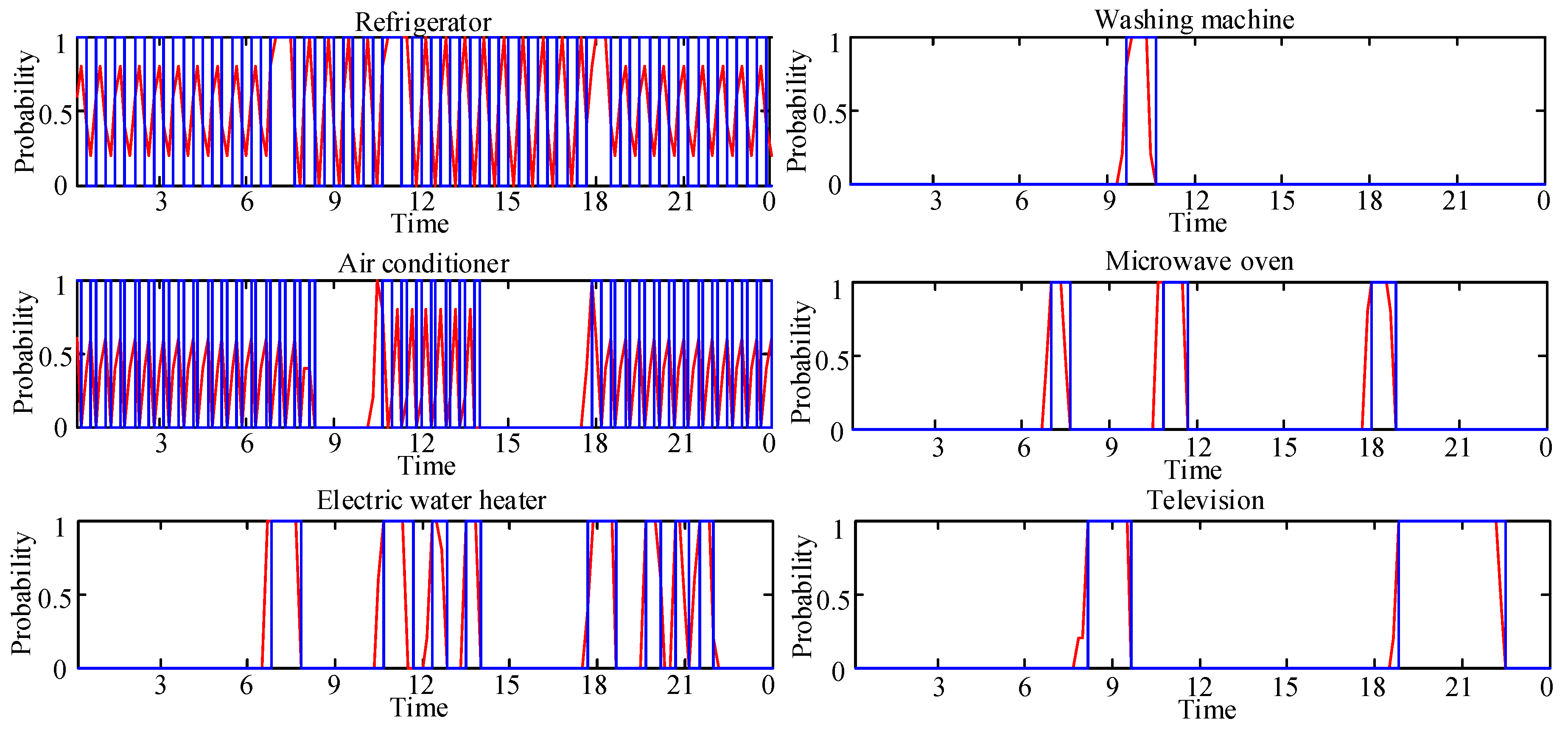
The electricity consumption behavior for household appliances on 31 July 2017 was predicted based on the similar historical days, and Figure 3 shows the working probability of six common household appliances at each sampling point. In the figure, the red curve is the predicted working probability of household appliances, and the blue curve is the actual working probability of household appliances. One can see that the predicted probability for these appliances is very similar to the actual working condition. For example, the refrigerator’s working condition is relatively stable, and it rotates between work and standby modes for 24 h. According to the predicted result, the refrigerator has a relatively long-running operation from 6:50 h to 7:20 h, between 10:40 h and 11:20 h, and between 17:40 h and 18:10 h, which is the same as the actual situation. It can be judged that this household uses the fridge frequently in each meal time period. In the prediction result, the air conditioner is in operation from 0:00 h to 8:00 h, from 10:10 h to 13:30 h, and from 17:30 h to 24:00 h, while the actual working condition of the air conditioner is from 0:00 h to 8:00 h, from 10:30 h to 13:40 h, and from 17:40 h to 24:00 h. One can see that there is a better forecasted result in the early morning and evening periods, and the overall prediction accuracy in the noon is up to 85%. Similarly, the forecasted results for the electric water heater, washing machine, microwave oven, and television also high overall prediction accuracies.
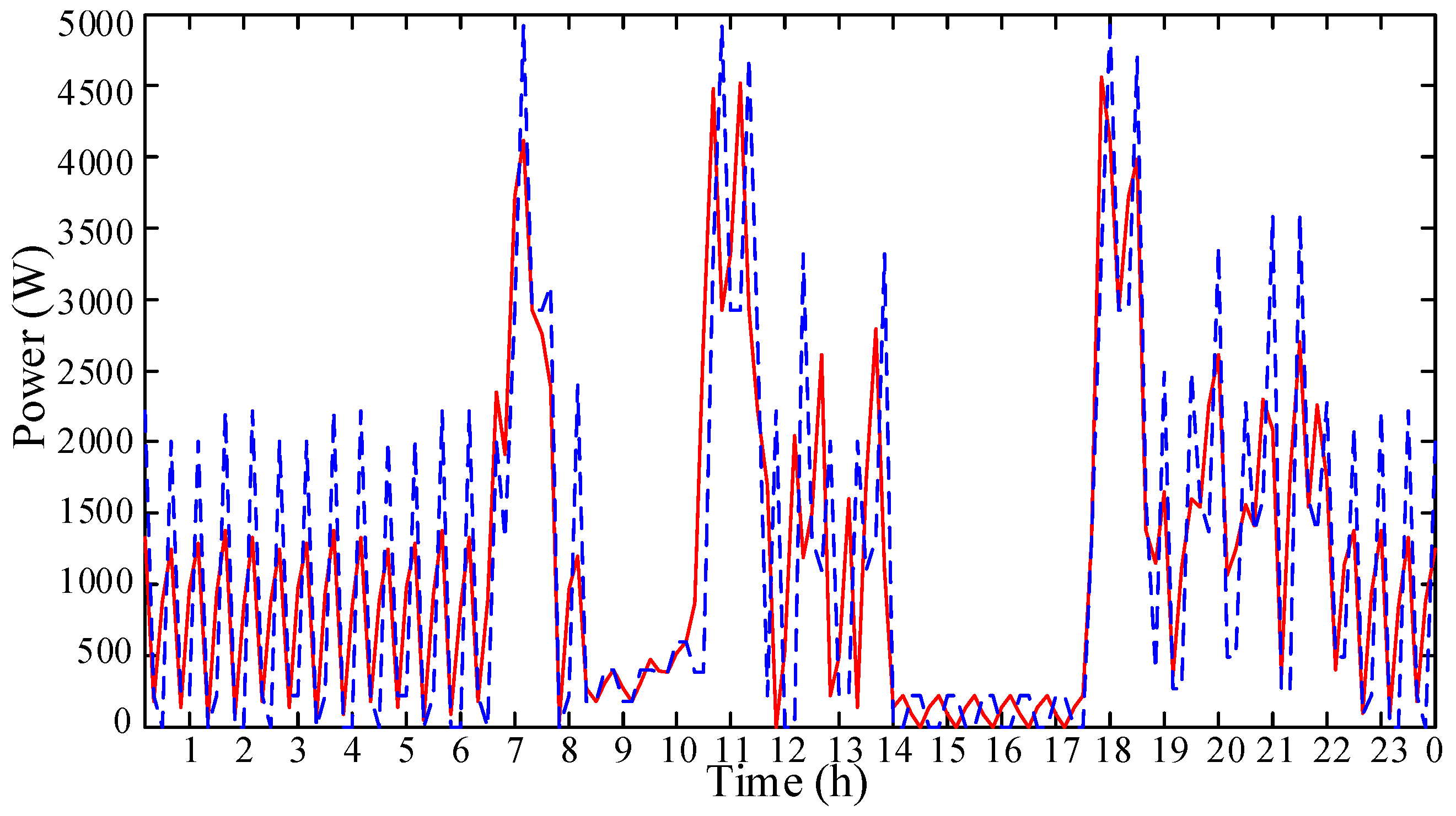
Based on the predicted results of all household appliances, the expected daily power of this household was obtained. Figure 4 shows the comparison result between the expected power and the actual power of this single household. From the red curve, one can see that the main consumption time for the household is from 6:30 h to 8:00 h, from 10:20 h to 11:50 h, from 17:30 h to 18:30 h, in which peak consumption is at 17:50 h with 4556 W, 11:00 h with 4520 W, 7:10 h with 4120 W, and off-peak consumption is from 8:30 h to 10:00 h and from 14:00 h to 17:40 h with about 200 W. Based on the actual profile in blue color, the comparison result shows that prediction error of peak consumption in the morning was 16.26%, at noon it was 7.39%, and in the evening it was 7.39%, and the prediction accuracy for the determination of peak consumption was 10 min. Therefore, the prediction results are in good agreement with the measured data, and can accurately predict each peak and valley time. Additionally, from 0:00 h to 8:00 h, due to the operation characteristics of the air conditioner, the expected power is different from the actual power, but the expected energy consumption is the same. Similarly, the time interval from 22:30 h to 24:00 h still has the same result.

5.2. Forecasting Result for Group Household

Generally, households in a community can be divided into different categories according to their energy consumption characteristics. Families in different categories will have different family member structures, and the forecasting accuracy will also be different. In our measured residential community, three categories exist: worker families, senior families, and senior + worker families. Therefore, in the forecasting process for group households, we firstly predicted the load in each category to show the effectiveness of the proposed approach, and then the load profile of group household was obtained by accumulating the consumption of all categories. In order to classify the group households precisely, the households in the community were clustered according to the peak consumption times and timetables of residents, such as the morning, noon, evening peak time, wake up time, and bedtime. In this paper, the adopted clustering method is fuzzy c-means clustering (FCM) [28,29,30]. Using the FCM algorithm, group households can be classified into different categories based on the consumption time information for each family. Additionally, the consumption time information for 64 households was collected and is shown in Table A2.
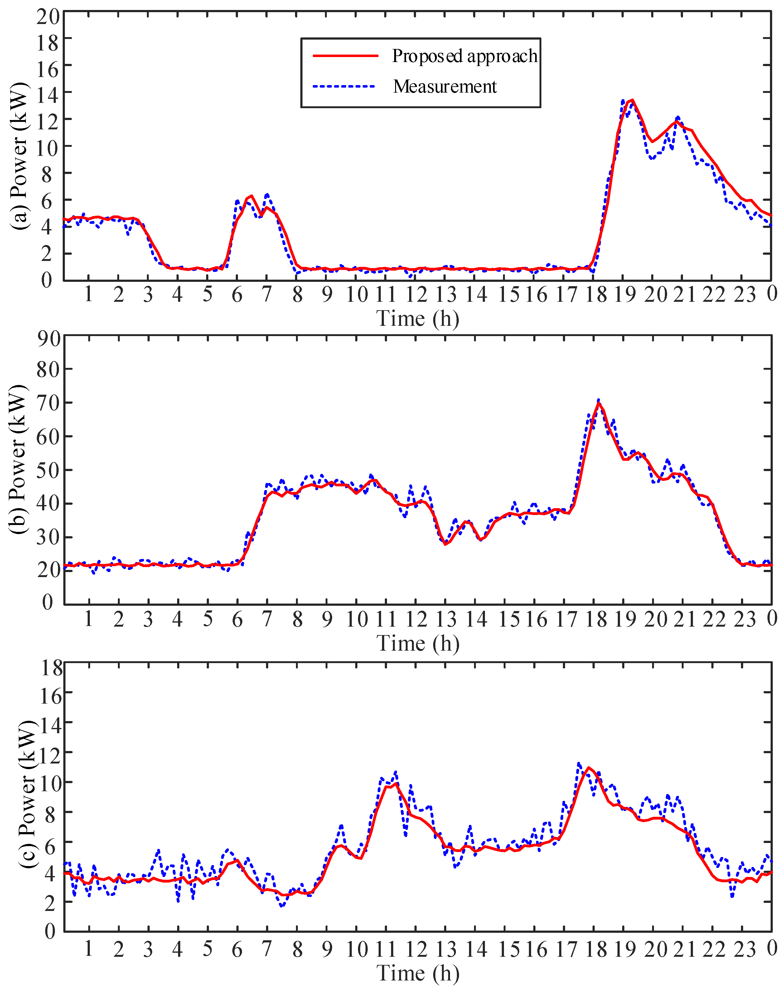
According to the household characteristic data, the clustering target is three categories (i.e., worker family, senior family, and senior + worker family) with FCM. The clustering results of the 64 households were as follows: 13 households are worker families (category 1), 40 households are senior + worker families (category 2), and 11 households are senior families (category 3). Then, based on the bottom-up forecasting approach, the energy consumption behavior of categories 1–3 was predicted, which is shown in Figure 5. By comparing the results, we can see that three categories of households have different energy consumption behaviors. This demonstrates that the proposed prediction model can reflect the electricity consumption characteristics of households in different categories. The worker family group has morning and evening peak times, where the evening peak time has a higher peak value and lasts for a longer period. The curve shows that this category has an centralized energy consumption time and the peak/valley difference is also obvious. Compared to the load profile of worker families, the energy consumption of the senior + worker family group is decentralized in the daytime, namely, the middle peak time lasts for a longer period, from 7:00 h to 18:00 h. The senior household group has a more distributed energy consumption time, in which there exists a small difference between the peak load and valley load. The curve shows that this category has less fluctuation than the other two categories. Moreover, from the aspect of prediction accuracy, one can see that in the result for the worker family, the predicted profile is coincident with the measured load profile most of the time, while for the senior family, the predicted profile has frequent fluctuation in the measured load. This demonstrates that the load profiles of worker families are easier to predict than those of senior families. The main reason for this is that users in the worker family have relatively fixed timetables, and they generally use appliances for the same purpose in a centralized time slot. For example, most worker families use kitchen appliances extensively for breakfast between 6:00–8:00 h during the workday, hence, the consumption behavior is easier to forecast. However, since senior members in the family have a more flexible consumption time, this will increase the randomness of consumption behavior on different days; hence, the predicted load profile of the measured load is the weakest.
Based on the forecasting result of the 3 categories, the load profile of whole residential community was obtained, which is shown in Figure 6. In order to show the effectiveness and efficiency of the proposed forecasting approach, a prediction result is also presented with a bottom-up formulation, but without the similar day extraction process. That is, the load profile was predicted via historical load dates from July 26 to 30 in the comparison approach. Figure 6a shows the prediction result, and Figure 6b,c show the relative errors between the predicted power and actual power. From the figures, we can see that the maximal absolute value of prediction error in the proposed approach was 12.3% at 13:20 h, and most of time, the prediction error was under 10%, while in the comparison approach, the maximal absolute value of prediction error was 20.0% at 17:10 h. In addition, from the relative error, one can see that the prediction result without the similar day extraction process hah a continuous large error (e.g., more than 10%) between 16:00 h and 19:00 h, which demonstrates that the comparison approach failed to give an accurate prediction for the evening peak moment. In addition, prediction errors in the peak value, valley value, and average value are presented in Table 2. This shows that in the critical moments, the proposed approach produces a great improvement from the prospect of prediction accuracy (e.g., 8% in peak moment, 4.2% in valley moment, and 3.4% in average value). Therefore, the proposed bottom-up modelling method is effective in the prediction of household load profiles. As for the feasibility of proposed approach in practice, the Matlab timer showed that the computing time of the whole forecasting process was 78.8 s, and the average computing time for each family was about 1.2 s. Note that, the forecasting algorithm was executed by MATLAB R2012b on the personal computer with Intel(R) Core(TM) i7-7700 [email protected] GHz and RAM 8.00 GB. Although the algorithm may have a longer running time for thousands of households on the personal computer, the running time will be reduced dramatically when the algorithm is performed on a computing server. Therefore, the proposed forecasting approach could be employed in reality.

5.3. Discussion on the Application of Proposed Approach

According to the above analysis, the proposed bottom-up approach was able to effectively predict the load profile of the residential community where consumption data was collected at the appliance level . However, since the collection work of bottom level data is a tremendous task, especially for the city with numerous residents, it is expected to that the collected data from one city will be applied to predict the consumption in another city with the proposed bottom-up approach. Generally, the data in one city can be applied to other cities with similar climates and economic levels. In order to measure the similarity degree among cities, a similarity feature vector can be employed:
Y = T R H V E ,
where T, R H , and V are the average air temperature, average relative air humidity, and average wind speed of a city, respectively; E is the economic level of a city. Furthermore, the factors are normalized in the similarity feature vector with the following formula:
T * = T / max T R H * = R H / max R H V * = V / max V E * = E / max E ,
where T * , R H * , V * , and E * are the normalized values. In addition, the similarity feature vector Y is replaced with normalized value ( Y * ). Using the vector of each city, we can obtain the degree of similarity between two cities by calculating the Euclidean distance:
l Y a * , Y b * = T a * T b * 2 + R H a * R H b * 2 + V a * V b * 2 + E a * E b * 2
s Y a * , Y b * = 1 1 + l Y a * , Y b * ,
where Y a * = T a * R H a * V a * E a * and Y b * = T b * R H b * V b * E b * are the similarity feature vectors of two cities, respectively; s Y a * , Y b * is the degree of similarity of two cities. Therefore, whether appliance data collected in one city can be used to another city can be determined according to the value of s Y a * , Y b * .

6. Conclusions

In this paper, a bottom-up forecasting framework was proposed to determine household load profiles, in which energy consumption behavior characteristics of each household appliance was regarded as the main building block. Furthermore, in order to enhance the performance of the forecasting process, a similar day extraction process was proposed to select the days most similar to the predicted day from numerous historical days. Using the appliance consumption data from similar historical days, the consumption behavior of group households can be more accurately predicted. In the case study, a set of data about the energy consumption of appliances and basic information (e.g., environment, event, household, and date) were collected from 1 July 2017 to 31 July 2017 in a residential group of 64 households. Using the collected data, a household load profile for July 31 was predicted with the proposed approach, and the results showed that the proposed bottom-up modelling method can predict different categories of families very well, including worker families, senior families, and senior + worker families. In addition, by comparing the results of the proposed approach and the bottom-up approach without the similar day extraction process, it was shown that the bottom-up modelling method considering similar day extraction will contribute to the prediction performance of the load profile.
Although the load profile predictions considered in this paper are only for residents, the forecasting framework could be applied to different scenarios with different electricity users, such as commercial users, highly localized power grids, and so on. In addition, the results in this paper could be extended in several directions. For example, the consumption power of household appliances was assumed to be the rated power in this paper; hence, research on the practical consumption model of appliances is worth studying. Furthermore, in Section 5.3, the selection standard for the degree of similarity value ( s Y a * , Y b * ) is an important factor that guarantees the prediction accuracy of the application of other cities; hence, it will be an important research direction in the future after obtaining the measured consumption data of multiple cities.

Author Contributions

B.G. contributed to developing the ideas of this research. X.L. and Z.Z. performed the research. All authors were involved in preparing this manuscript.

Funding

This research received no external funding.

Conflicts of Interest

The authors declare no conflict of interest.

Appendix A

Table A1. Basic information in July 2017.
DateHumidityTemperatureWind SpeedWeekday TypeMajor Event
1 July 20174528660
2 July 201770331270
3 July 20174726810
4 July 20174828620
5 July 201751301030
6 July 20173330740
7 July 20174032850
8 July 20174532860
9 July 20177230770
10 July 201781341210
11 July 20176532820
12 July 201775301230
13 July 201773301040
14 July 201771301050
15 July 20176032560
16 July 20176132370
17 July 20176032910
18 July 20175232820
19 July 20176032730
20 July 201778301140
21 July 20176530850
22 July 20176134760
23 July 20174734870
24 July 201771351110
25 July 201760341020
26 July 20174332930
27 July 20174834640
28 July 201784361250
29 July 201777361160
30 July 201779321270
31 July 20176033810
Table A2. Consumption time information for each family.
FamilyMorningNoonEveningWakeBedFamilyMorningNoonEveningWakeBed
142651083713833376510634126
241641093913934426311038135
34401134214335446211139137
443701134214136416811539137
543691124314237456310939139
64401134214238456310939137
73769108351263944011242144
844661133513740436211040139
944621074113741426410740135
1043631094013542376810735125
114501114314243436511240137
123565106311304445011442144
1343661093613445426411240137
1442651084013746346410733120
1542681154114247436710839136
1643641104013748406711138134
174501144314449426411340138
184464110351355045011543143
1938681083512651376810935124
2043641074013652406310939136
2143651093913853396611240135
2239701103812554436711139134
234465107411365544011842143
244401124214356436411040133
254363107411325743011643144
2643641073913358446510940135
274501154214459436611040134
283668107341226044011341141
294401184114061366610734127
3042671144013862446410841132
3143641084013463416911038133
3245641094013264356511134124

References

  1. Shi, J.; Lee, W.; Liu, X. Generation scheduling optimization of wind-energy storage system based on wind power output fluctuation features. IEEE Trans. Ind. Appl. 2018, 54, 10–17. [Google Scholar] [CrossRef]
  2. Capozzoli, A.; Piscitelli, M.; Brandi, S. Mining typical load profiles in buildings to support energy management in the smart city context. Energy Procedia 2017, 134, 865–874. [Google Scholar] [CrossRef]
  3. Mediwaththe, C.; Stephens, E.; Smith, D. Competitive energy trading framework for demand-side management in neighborhood area networks. IEEE Trans. Smart Grid 2017, 1–10. [Google Scholar] [CrossRef]
  4. Gajowniczek, K.; Zabkowski, T. Electricity forecasting on the individual household level enhanced based on activity patterns. PLoS ONE 2017, 12, e0174098. [Google Scholar] [CrossRef] [PubMed]
  5. Chuan, L.; Ukil, A. Modeling and validation of electrical load profiling in residential buildings in Singapore. IEEE Trans. Power Syst. 2015, 30, 2800–2809. [Google Scholar] [CrossRef]
  6. Swan, L.G.; Ugursal, V.I. Modeling of end-use energy consumption in the residential sector: A review of modeling techniques. Renew. Sustain. Energy Rev. 2009, 13, 1819–1835. [Google Scholar] [CrossRef]
  7. Jardini, J.A.; Tahan, C.M.V.; Gouvea, M.R. Daily load profiles for residential, commercial and industrial low voltage consumers. IEEE Trans. Power Deliv. 2000, 15, 375–380. [Google Scholar] [CrossRef]
  8. Hoverstad, B.A.; Tidemann, A.; Langseth, H. Short-term load forecasting with seasonal decomposition using evolution for parameter tuning. IEEE Trans. Smart Grid 2015, 6, 1904–1913. [Google Scholar] [CrossRef]
  9. Thouvenot, V.; Pichavant, A.; Goude, Y. Electricity forecasting using multi-stage estimators of nonlinear additive models. IEEE Trans. Power Syst. 2016, 31, 3665–3673. [Google Scholar] [CrossRef]
  10. McLoughlin, F.; Duffy, A.; Conlon, M. Characterising domestic electricity consumption patterns by dwelling and occupant socio-economic variables: An Irish case study. Energy Build. 2012, 48, 240–249. [Google Scholar] [CrossRef]
  11. Wang, C.; Grozev, G.; Seo, S. Decomposition and statistical analysis for regional electricity demand forecasting. Energy 2012, 41, 313–325. [Google Scholar] [CrossRef]
  12. Dordonnat, V.; Koopman, S.J.; Ooms, M. An hourly periodic state space model for modelling French national electricity load. Int. J. Forecast. 2008, 24, 566–587. [Google Scholar] [CrossRef] [Green Version]
  13. Stephen, B.; Mutanen, A.J.; Galloway, S. Enhanced load profiling for residential network customers. IEEE Trans. Power Deliv. 2014, 29, 88–96. [Google Scholar] [CrossRef]
  14. Nagbe, K.; Cugliari, J.; Jacques, J. Short-Term Electricity Demand Forecasting Using a Functional State Space Model. Energies 2018, 11, 1120. [Google Scholar] [CrossRef]
  15. Capasso, A.; Grattieri, W.; Lamedica, R. A bottom-up approach to residential load modeling. IEEE Trans. Power Syst. 1994, 9, 957–964. [Google Scholar] [CrossRef]
  16. Marszal-Pomianowska, A.; Heiselberg, P.; Larsen, O.K. Household electricity demand profiles-A high-resolution load model to facilitate modelling of energy flexible buildings. Energy 2016, 103, 487–501. [Google Scholar] [CrossRef]
  17. Widen, J.; Nilsson, A.M.; Wackelgard, E. A combined Markov-chain and bottom-up approach to modelling of domestic lighting demand. Energy Build. 2009, 41, 1001–1012. [Google Scholar] [CrossRef]
  18. Paatero, J.V.; Lund, P.D. A model for generating household electricity load profiles. Int. J. Energy Res. 2006, 30, 273–290. [Google Scholar] [CrossRef] [Green Version]
  19. Fischer, D.; Hartl, A.; Wille-Haussmann, B. Model for electric load profiles with high time resolution for German households. Energy Build. 2015, 92, 170–179. [Google Scholar] [CrossRef]
  20. Fischer, D.; Wolf, T.; Scherer, J. A stochastic bottom-up model for space heating and domestic hot water load profiles for German households. Energy Build. 2016, 124, 120–128. [Google Scholar] [CrossRef]
  21. Singh, S.; Yassine, A. Big data mining of energy time series for behavioral analytics and energy consumption forecasting. Energies 2018, 11, 452. [Google Scholar] [CrossRef]
  22. Richardson, I.; Thomson, M.; Infield, D. Domestic electricity use: A high-resolution energy demand model. Energy Build. 2010, 42, 1878–1887. [Google Scholar] [CrossRef] [Green Version]
  23. Widen, J.; Wackelgard, E. A high-resolution stochastic model of domestic activity patterns and electricity demand. Appl. Energy 2010, 87, 1880–1892. [Google Scholar] [CrossRef]
  24. Lin, S.; Huang, N.; Zhao, L. Domestic daily load curve modeling based on user behavior. Electr. Power Constr. 2016, 37, 114–121. [Google Scholar]
  25. Wei, H.; Su, Z.; Yao, G. The Short-Term Load Forecasting Based on Similar Day and PSO-NN Model with Human Body Comfortable Indicator Vector. Power Syst. Clean Energy 2016, 32, 135–139. [Google Scholar]
  26. Angelos, E.W.S.; Saavedra, O.R.; Cortes, O.A.C. Detection and identification of abnormalities in customer consumptions in power distribution systems. IEEE Trans. Power Deliv. 2011, 26, 2436–2442. [Google Scholar] [CrossRef]
  27. Ma, Z.; Yan, Z.R.; Nord, N. A variation focused cluster analysis strategy to identify typical daily heating load profiles of higher education buildings. Energy 2017, 134, 90–102. [Google Scholar] [CrossRef]
  28. Chicco, G.; Napoli, R.; Piglione, F. Comparisons among clustering techniques for electricity customer classification. IEEE Trans. Power Syst. 2006, 21, 933–940. [Google Scholar] [CrossRef]
  29. Ferraro, P.; Crisostomi, E.; Tucci, M. Comparison and clustering analysis of the daily electrical load in eight European countries. Electr. Power Syst. Res. 2016, 141, 114–123. [Google Scholar] [CrossRef]
  30. Panapakidis, I.; Asimopoulos, N.; Dagoumas, A. An Improved Fuzzy C-Means Algorithm for the Implementation of Demand Side Management Measures. Energies 2017, 10, 1407. [Google Scholar] [CrossRef]
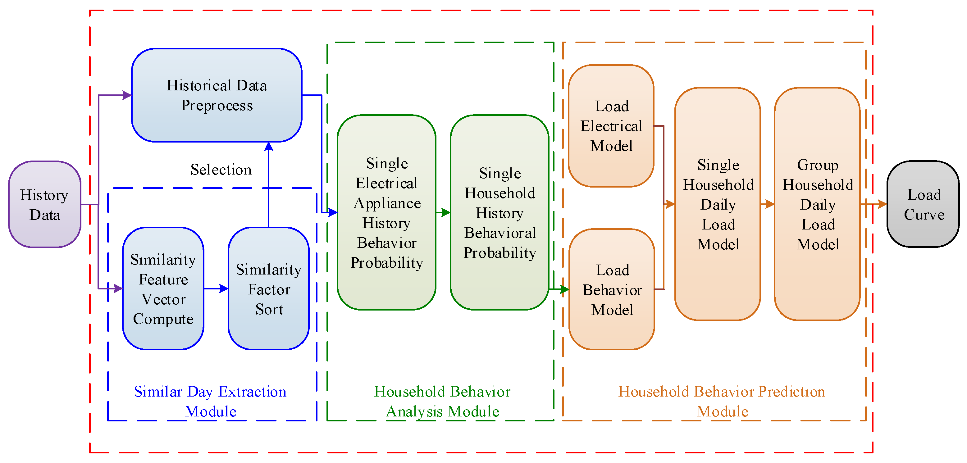
Figure 1. Forecasting framework of group household electricity consumption.
Energies 11 02112 g001
Figure 2. Similarity curve among historical days and predictive day.
Energies 11 02112 g002
Figure 3. Consumption behavior of household appliances.
Energies 11 02112 g003
Figure 4. Expected power of a single household.
Energies 11 02112 g004
Figure 5. Forecasting results for three categories of household: (a) worker family; (b) senior + worker family; (c) senior family.
Energies 11 02112 g005
Figure 6. Prediction results for the residential community: (a) is the forecasting power; (b) is the error between the proposed approach and the measurement; (c) is error the between the comparison approach and the measurement.
Energies 11 02112 g006
Table 1. Power of partial household appliance.
AppliancePower (W)AppliancePower (W)
Fluorescent lamp90Air conditioner2000
Washing machine380Electric water heater1100
Microwave oven900Television180
Refrigerator220Rice cooker500
Table 2. Prediction errors of the peak, valley, and average power values.
Parameter P max P min P av
Measurement (W)85,76024,18845,824
Proposed approach (W)88,79425,34846,366
Comparison approach (W)95,60526,36247,946
Proposed approach error (%)3.54.81.2
Comparison approach error (%)11.59.04.6