Impact of Demand-Side Management on the Reliability of Generation Systems


1
School of Electrical and Electronic Engineering, Universiti Sains Malaysia (USM), Nibong Tebal 14300, Penang, Malaysia
2
Inspector General Office, Ministry of Water Resources, Filastin 10046, Baghdad, Iraq
*
Author to whom correspondence should be addressed.
Energies 2018, 11(8), 2155; https://doi.org/10.3390/en11082155
Submission received: 1 August 2018
/
Revised: 13 August 2018
/
Accepted: 15 August 2018
/
Published: 17 August 2018
(This article belongs to the Section F: Electrical Engineering)
Abstract
:The load shifting strategy is a form of demand side management program suitable for increasing the reliability of power supply in an electrical network. It functions by clipping the load demand that is above an operator-defined level, at which time is known as peak period, and replaces it at off-peak periods. The load shifting strategy is conventionally performed using the preventive load shifting (PLS) program. In this paper, the corrective load shifting (CLS) program is proven as the better alternative. PLS is implemented when power systems experience contingencies that jeopardise the reliability of the power supply, whereas CLS is implemented only when the inadequacy of the power supply is encountered. The disadvantages of the PLS approach are twofold. First, the clipped energy cannot be totally recovered when it is more than the unused capacity of the off-peak period. The unused capacity is the maximum amount of extra load that can be filled before exceeding the operator-defined level. Second, the PLS approach performs load curtailment without discrimination. This means that load clipping is performed as long as the load is above the operator-defined level even if the power supply is adequate. The CLS program has none of these disadvantages because it is implemented only when there is power supply inadequacy, during which the amount of load clipping is mostly much smaller than the unused capacity of the off-peak period. The performance of the CLS was compared with the PLS by considering chronological load model, duty cycle and the probability of start-up failure for peaking and cycling generators, planned maintenance of the generators and load forecast uncertainty. A newly proposed expected-energy-not-recovered (EENR) index and the well-known expected-energy-not-supplied (EENS) were used to evaluate the performance of proposed CLS. Due to the chronological factor and huge combinations of power system states, the sequential Monte Carlo was employed in this study. The results from this paper show that the proposed CLS yields lower EENS and EENR than PLS and is, therefore, a more robust strategy to be implemented.
1. Introduction
Electrical power grids must be highly integrated to cope with the uncertainties in load and supply. The electric utility industry is obligated to supply efficient and reliable electric services to customers; therefore, the reliability of power supply is demanded by the present-day society. However, satisfying this demand has become challenging due to new trends and complex technologies, environmental constraints and load growth [1]. One of the investigations on power system reliability is the adequacy study of generation systems, and it is concerned only with the capability to satisfy customer demands [2]. In this study, transmission and distribution systems were not considered and assumed fully reliable. Although system reliability can be maintained/increased by increasing investment into the system, the investment cost must be justified by the value of reliability improvement, representing the conflicting constraints that must be considered [2,3]. Thus, identifying an optimal managerial decision at the planning phases is beneficial for ensuring customer satisfaction at all times.
In response to the above, utilities worldwide consider demand-side management (DSM) programmes as an alternative for power generation because of their tremendous technical, environmental and economic impacts. DSM programmes are initiatives implemented by electricity utilities to encourage consumers to adopt procedures and practices that are advantageous from system and customer viewpoints [4,5,6,7]. The various techniques of DSM programmes are valley filling, peak clipping, load shifting, flexible load shape, energy efficiency and strategic load growth [4,6,8]. Research has shown that, instead of expanding the generation systems, DSM programmes can be implemented to achieve the same level of power system reliability [9]. In view of the suggestion, an accurate evaluation of the DSM impact on generation system adequacy is important [10].
The load-shifting programme, as one of the DSM techniques, can be classified into preventive load shifting (PLS) and corrective load shifting (CLS) [11]. The PLS programme is implemented usually when the system is under increased risk, when the electrical power system is in jeopardy or at times of high electricity prices, whereas the CLS programme is implemented immediately after the inadequacy of power supply is encountered [11]. There are two major limitations and barriers to the implementation of PLS: the unnecessary clipping of load in the healthy operation duration, and the amount of the scheduled recovered energy may be greater than the pre-specified peak value, contributing to energy not recovered (ENR).
Considerable works have been performed for the adequacy assessment of generation systems that incorporate DSM. The impact of load shifting on generation system adequacy considering load uncertainty was proposed [12,13]. The load-shifting impact on production cost and the adequacy of power supply was assessed [14,15]. Load shifting was considered for optimising load demand [16]. Load-shifting techniques were integrated with shutdowns and start-ups of generation units to evaluate the advantages of load levelling and the cycling costs of thermal generation units [17]. The operational benefits of DSM for a fuel cell power plant was assessed [18]. The economic and environmental effects after integrating DSM and supply-side management strategies were studied [19]. Peak-clipping technique was modelled to evaluate the worth of DSM in the planning framework of generation systems [20]. Load-shifting technique was analysed by considering the duty cycle of generation units, outage postponability, unit commitment policy, operating reserve, the starting time of generation units, planned outages and running and starting failure repairs [10,21]. Load-shifting technique was assessed by considering two interconnected systems and energy storage systems [22]. However, most of the above-mentioned studies have ignored the impact of each DSM technique. This issue was resolved in [23] by modelling all DSM techniques, except flexible load shaping. In this study, the impact of electricity on the total societal costs and on the planning reserve margin was evaluated. The integration of demand- and supply-side planning into reliability worth and its cost analysis was investigated as well.
However, none of the literature above has considered the CLS model before. A study assessing the impact of CLS comparing to PLS on the adequacy of generation system is needed. The duty cycle and failure initiation of peaking and cycling generation units, planned maintenance and load forecast uncertainty (LFU) should be considered as well for a more realistic evaluation. As such, this presents a gap that this paper intends to fill and the contributions of the paper are summarised below:
- The CLS program is modelled for the first time to simulate the dynamic load shifting strategy during the inadequacy of power supply. The superiority of the CLS program is highlighted by comparing its performance with the well-known PLS program.
- A new index known as the expected-energy-not-recovered (EENR) is proposed to measure the inability of both the PLS and CLS in recovering the curtailed load.
- The modelling of the generation system in this study considers the two-state, four-state, and planned maintenance models. Load forecast uncertainty (LFU) is considered for the load model. The reliability impacts of these models are considered in PLS and CLS programs and their reliability performances are compared.
Results from this paper show that CLS is more effective than PLS in terms of improving the reliability of power supply. The remainder of this paper is organised as follows. Methodologies of the adequacy planning of generation systems and load-side are given in Section 2. Results and discussions are provided in Section 3. Conclusions are given in Section 4.
2. Methodology
2.1. Generation System Model
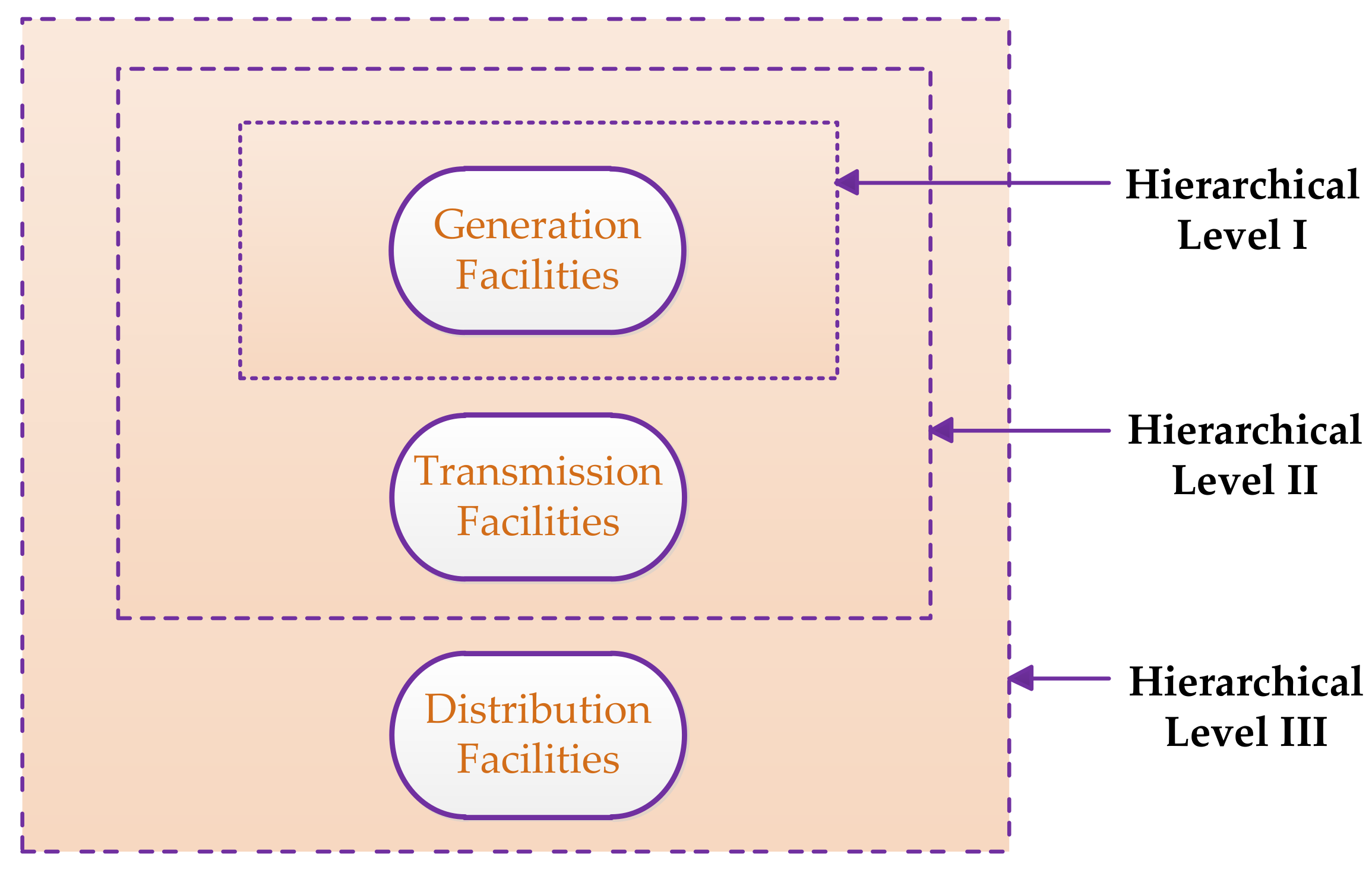
Electric power systems are categorised into three hierarchical levels (HLs), as shown in Figure 1. HLI considers only the reliability of generation systems. The transmission and distribution networks are considered fully reliable in this level and there are no constraints in delivering electricity to consumers. HLII jointly considers the reliability of generation and transmission systems. HLIII considers the reliability of distribution system on top of HLII.
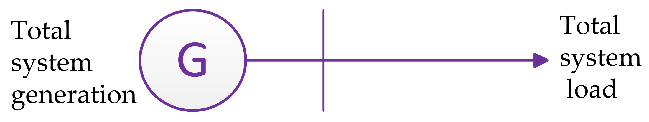
In the context of electrical network, the reliability evaluation of HL1 is illustrated in Figure 2 where only the ability of the generation system to meet load demand is considered [2,3]. When the load demand is more than the generation level, load curtailment is recorded. When this value is sampled over multiple situations, considering various combinations of generator availabilities, and taking the average values, the expected-energy-not-served (EENS) index is obtained.
In this study, the sequential Monte Carlo simulation (due to chronological load model; see Section 2.2) was performed to determine the EENS and is calculated as follows [2,3]:
where is the probability of system state , is the loss of load for system state , and is the number of simulation year.
2.1.1. Two-State Model
Generation units are divided into three types—base load, cycling and peaking units. Base load units operate consistently to generate the electrical power needed to satisfy base load demand. These units are the most economical to operate and stop only for maintenance or unplanned outages. Peaking units operate only during high demand when load level surpasses the power supply of base load units. These units have a much higher production cost than base and cycling units. Due to this, the duty cycle of peaking units is shorter than base load units.
In the two-state model, all generation units transit only between up and down states regardless of the types of generators, as shown in Figure 3. The transition rates between up and down states in Figure 3 conform to the common assumption that they are constant due to its underlying exponential distribution.
As a result, the mean-time-to-failure (MTTF) and mean-time-to-repair (MTTR) are taken as the reciprocal of the failure and repair rates, respectively, and are constant, as shown in Equations (2) and (3). Then, the random values of time-to-failure () and time-to-repair () are obtained from Equations (4) and (5).
where is the uniformly distributed random number between [0, 1], is the failure rate, and is the repair rate.
2.1.2. Four-State Model
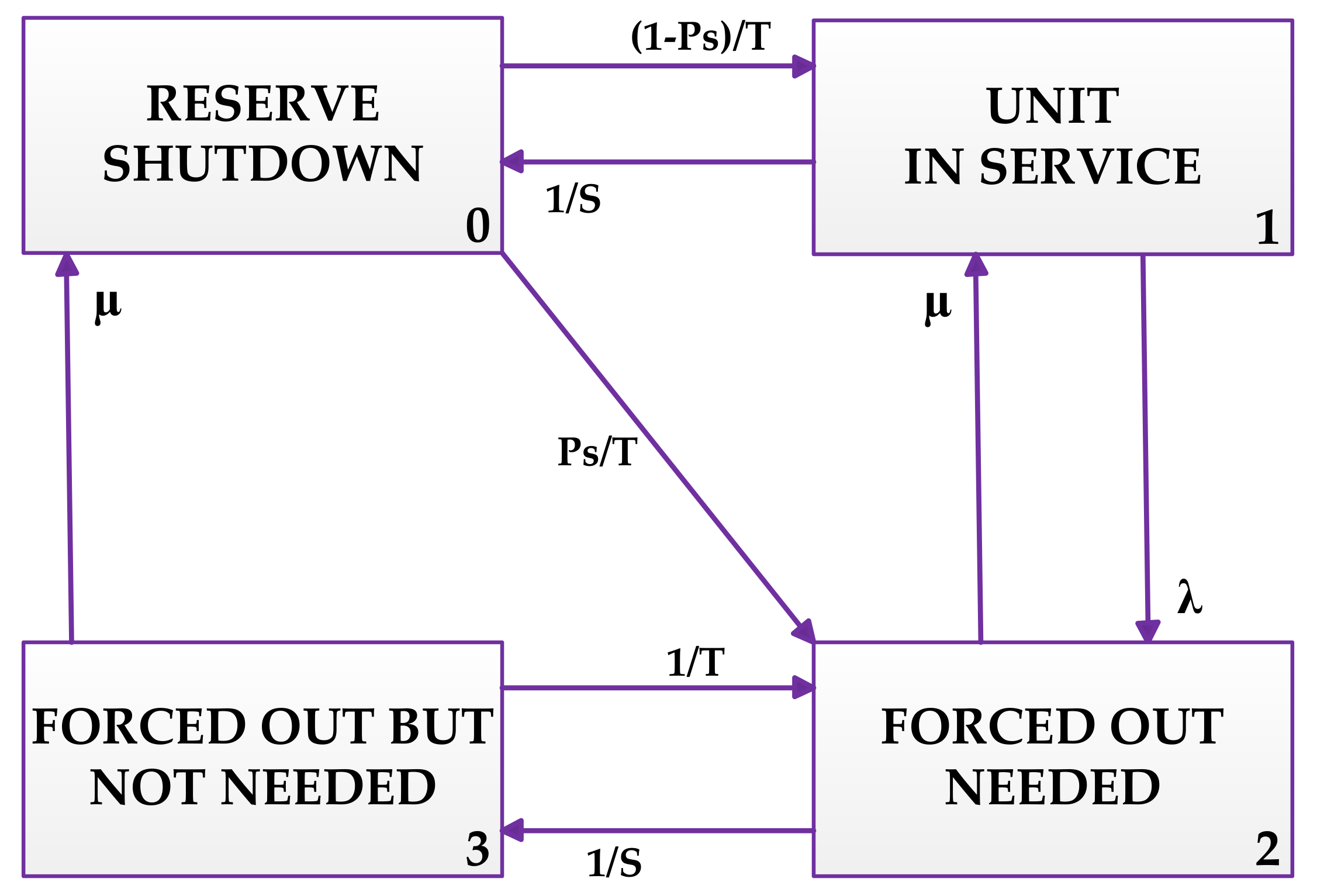
The two-state model cannot be properly used to model peaking and cycling generation units as they may not be needed when out of service due to unplanned outage. Moreover, when they are in service, periods of service may be interrupted by reserve shutdown. To deal with this issue, the IEEE task group on models for peaking and cycling units proposed the four-state model [24], as shown in Figure 4.
The figure shows that peaking and cycling service units have four states:
- Reserve shutdown state: The generation unit is shutdown but ready for loading.
- Service state: The generation unit is in operating condition.
- Forced out needed: The generation unit is in down state and in need.
- Forced out not needed: The generation unit is in down state and not needed.
Figure 4 also shows the parameters used to describe the transition among the different states. is the average reserve shutdown time amongst periods of need, excluding scheduled outage; is the average in-need time per occasion of demand; and is the probability of a starting failure causing all or part of the load unserved.
Throughout the year, peaking and cycling generation changes their status very often, as illustrated in Figure 4. The transition from State (0) to State (1) is represented by ; this rate is usually so small that peaking load units are needed only for a short period along the year (e.g., 50 h out of 7836 h). The period of being in reserve is usually much greater than the period of being in service. Therefore, the transition from State (1) to State (0) is represented by (1/), and, thus, this transition is greater than the transition from State (0) to State (1). The transition from State (0) to State (2) is represented by . The probability of a starting failure is considered only in the transition from State (0) to State (1) and from State (0) to State (2), as both transitions require the initiation to start peaking load units. The transition between State (1) and State (2) is the same as the two-state model. Down state is divided into two states, namely, needed and not needed. The transition from State (2) to State (3) is represented by , and it is the same as the transition from State (1) to State (0). The transition from State (3) to State (2) is represented by . The transition from State (3) to State (0) is represented by the repair rate (), and transition from State (0) to State (3) is unavailable because forced-out and not-needed state has no impact on the available generation level. Transition from State (2) to State (0) is unavailable as well because forced-out and needed state cannot transit to reserve shutdown state.
The simulation process of the four-state model is explained as follows:
- The total available capacity of base units is calculated after accumulating the and of all base units according to Equations (4) and (5).
- Chronological load is intersected with base units of available capacity to determine the needs (corresponding to ) for peaking and cycling units.
- Available capacity of each peaking and cycling unit is calculated using the two-state model initially, then modified using the following:where is the unit available capacity of the peaking and cycling unit and is the corresponding unit capacity. From Equation (6), if the random number is greater or equal to , the unit is considered start-up, otherwise it fails. Generators in the period of reserve shutdown (corresponding to ) are in the up state.
- Corresponding units of available capacity is accumulated and added to the base units of available capacity to form total system available capacity.
- Chronological load is subtracted from total system available capacity to determine the amount of curtailed energy and duration of loss of the load.
2.1.3. Scheduled Maintenance
Maintenance can be planned and unplanned [3]. In planned maintenance, the operation of generation units is scheduled to ensure sufficient power supply while optimising maintenance cost. In unplanned maintenance, generation units are usually out of service due to failures. When planned maintenance is considered, the risk level is approximately compounded because of the reduction in reserve margin at different times of the year [25]. Various scheduled plans have been presented in the literature before. The levelled risk criteria of the IEEE-reliability test system (RTS) describes a common scheduled plan and it is used in this study [25,26]. In this plan, the planned maintenance of generation units is arranged to minimise system risk. The IEEE-RTS generation unit capacities and their schedule plan are shown in Table 1 [25,26]. In this table, generation units are scheduled on a weekly basis depending on its capacity.
2.2. Demand-Side Management
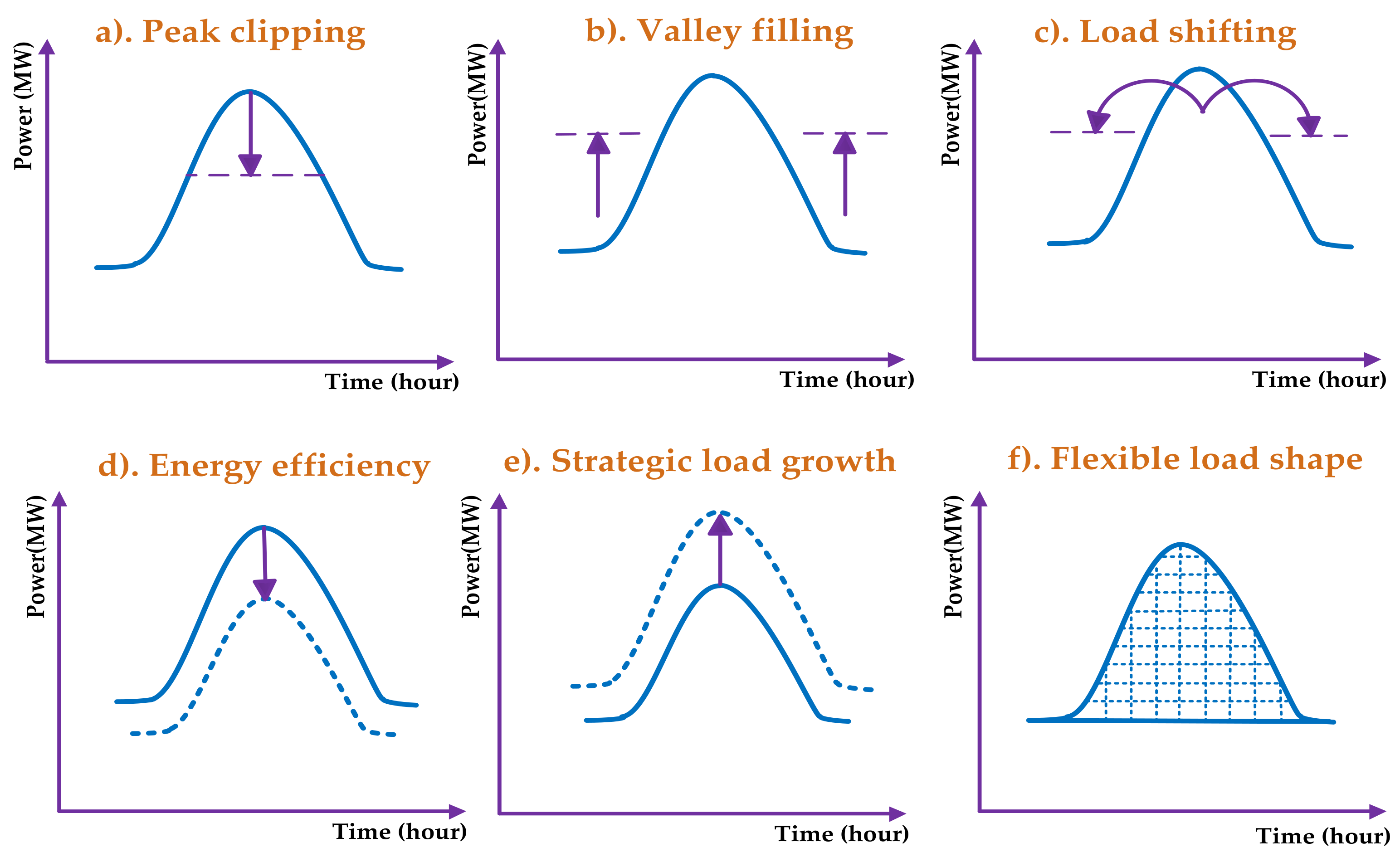
DSM is an initiative implemented by electric utilities to encourage consumers to adopt practices that are advantageous from system and customer views [4,5,6,7]. This initiative includes analysis, planning and implementation of utility activities to affect load shapes in either time pattern or magnitude [27]. The most important features of DSM programmes are maintaining the reliable performance of electrical power systems and improving the economic efficiency of the systems. Other DSM benefits involve maintaining voltage stability and transmission congestion, increasing the flexibility of planned maintenance, balancing energy resource and mitigating the drawbacks posed by the intermittency of renewable energy sources [11]. The various DSM techniques are shown in Figure 5 [4,6,8]. Valley filling involves building loads during the off-peak load curve period [7]. Peak clipping refers to the reduction in on-peak load [4]. Load shifting refers to the combination of peak-clipping and valley-filling measures—loads are clipped from on-peak period and recovered during off-peak period [6]. Flexible load shape refers to particular tariffs with opportunities to flexibly control consumer equipment [6,28]. Energy efficiency refers to lessening the total load demand by enhancing the efficiency of energy use. Strategic load growth is the increase in electrical energy [4]. This paper focuses onto the implementation of load shifting and will be discussed in detail next.
2.2.1. Load-Shifting Model
Load shifting is a combination of peak-clipping and valley filling measures and the full cycle of this technique is considered 24 h in this study. The curtailed load that cannot be filled within the considered period (24 h) is considered lost. Formally, the mathematical model of peak clipping is given in Equations (7) and (8), while Equations (9) and (10) describe the mathematical model of the valley filling measure [23].
where is the original demand of the system; and are the modified system load curves which result from implementing a load-shifting activity; is the pre-specified peak load level that cannot be exceeded; is the percentage of energy recovery during off-peak hours and its range is ; and are the first and last hour, respectively, when the original load is greater than (); and are the first and last hour, respectively, for the recovery of energy during off-peak hour; and is the duration given by the difference between and .
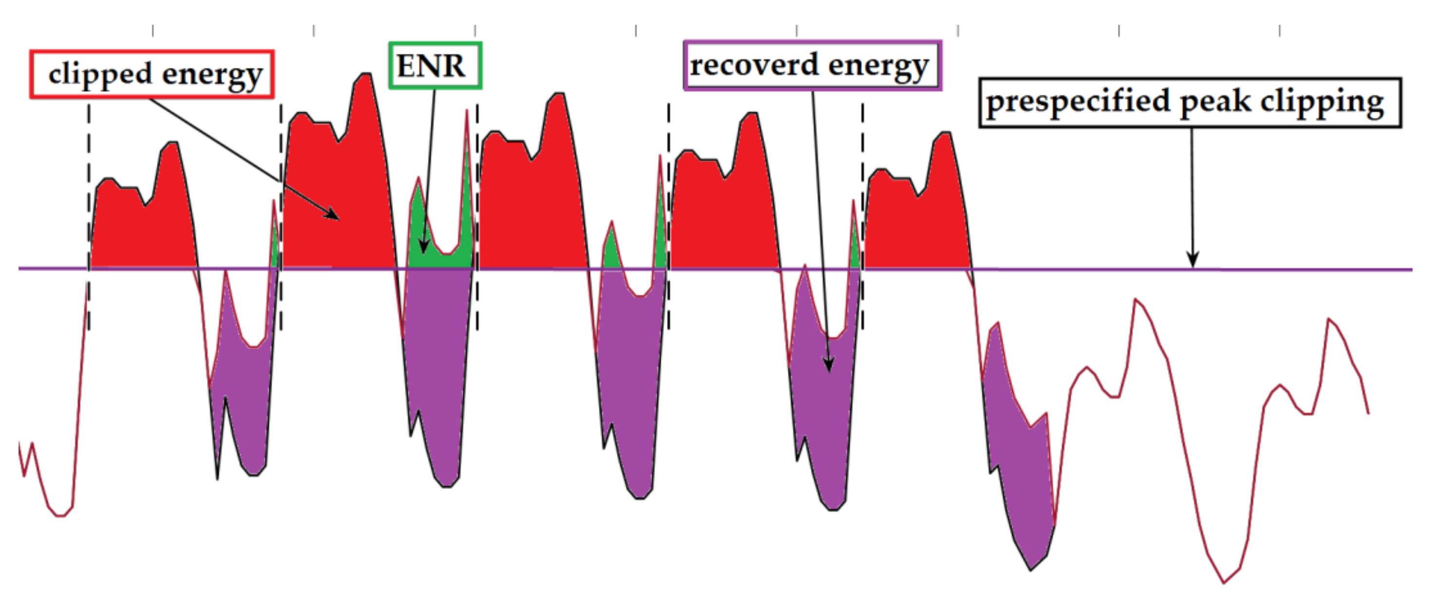
The disadvantages of PLS are the unnecessary clipping of load despite normal operation and the recovered energy may be greater than the pre-specified peak level. The unrecovered energy is called the energy not recovered (ENR), which is illustrated in Figure 6 for the case of PLS program. The figure shows that the ENR is obtained by calculating the difference between the pre-specified peak level and the scheduled energy for recovery. A negative value indicates there is ENR and vice versa.
The CLS technique is modelled as follows:
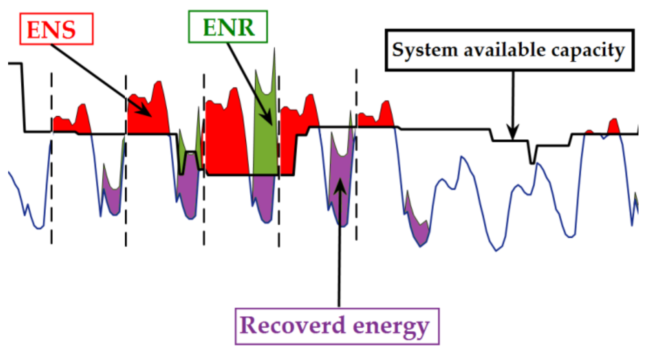
where is the first modified load curve after subtracting the instantaneous energy not supplied () from the original load. is the energy that must be shed during the period of inadequacy of power supply. The recovery of curtailed energy is considered only for the same day of load curtailment. In this study, it was assumed that the portion of the system load that is equal or more than the average curtailed energy per interruption is under the direct control of the system operators, and they are allowed to completely or partially shift the load during this time. However, the recovery of energy curtailment due to the random failures of generators is not guaranteed. Figure 7 illustrates the operation of the CLS program.
The main difference between PLS and CLS is in the threshold that is used to necessitate the load shifting operation. In PLS, as shown in Figure 6, load shifting is performed based on the pre-specified peak level. However, in CLS, as shown in Figure 7, load shifting is performed only when the system available generation capacity is lower than the load level.
The load shifting model of CLS is given as follows:
where is the second modified load curve after recovering the curtailed load from Equation (11); is the amount of added energy to each hour of recovery period; is the energy not recovered at each hour of energy recovery period; is the percentage of energy recovery and its range is ; is the first time during the day when the original load exceeds the system available capacity; is the last time during the day when the original load becomes equal or less than system available capacity; and are the starting and ending times for the off-peak recovery of energy; is the difference between and ; is the instantaneous system available capacity; is the expected energy not recovered; and is the number of simulation years.
2.2.2. Load Forecast Uncertainty
LFU considers the uncertainty of load level and it accounts for the possibility of the load to go above or below fixed load. Hence, uncertain future load requires a higher capacity reserve than fixed load [29].
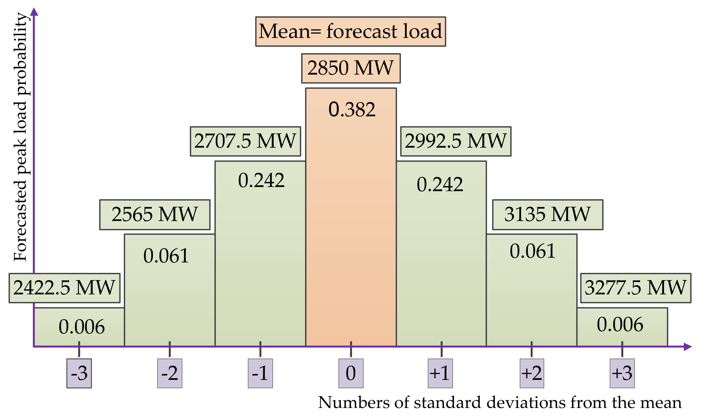
LFU has been modelled using a normal distribution before and this method is adopted in this paper [29]. In this method, the distribution mean represents the forecasted peak load. The distribution is also divided into a discrete number of intervals. In this study, the normal distribution was divided into seven discrete intervals with a standard deviation of 5% [2]. In other words, the difference in each interval class is 5%, equivalent to 142.5 MW. The probability of each interval was evaluated as the area under the density function, as shown in Figure 8 [30,31].
The reliability of the generation system incorporating LFU model is calculated as follows:
- Load level is selected based on the standard deviation from mean (peak level). Each load level is obtained by multiplying the peak value by the percentage of uncertainty. This value is added to the peak value to represent the increase in peak uncertainty or subtracted from peak to represent the decrease in peak uncertainty.
- The load level is multiplied by the probability that the load level occurs to obtain the weighted values for each level.
- The sum of all weighted load is the corresponding reliability index for the forecast load.
Table 2 summarises the above procedure for calculating the reliability index when LFU is considered.
2.3. Overview of Methodology
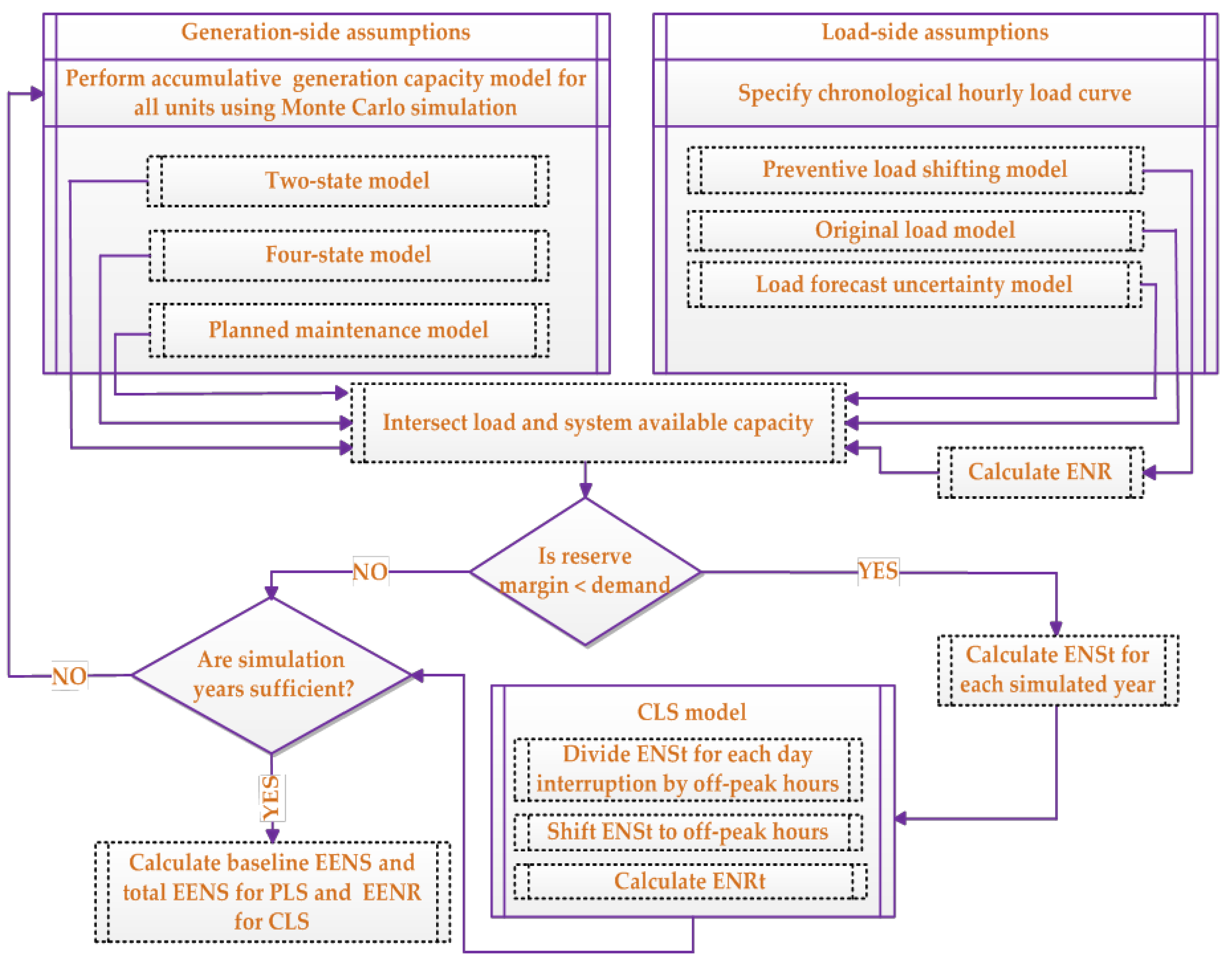
Figure 9 shows the flowchart of the proposed methodology for assessing the adequacy of the generating system by considering PLS, CLS, LFU and planned maintenance using two-state and four-state models. This figure shows that the algorithm has multiple models in load and generation sides. The algorithm process involves the following steps:
- Step 1:
- Specify the chronological hourly load curve.
- Step 2:
- Model the load as one of the following cases:
- Case 1:
- Original load, without any consideration.
- Case 2:
- Preventive load-shifting scenarios (peak clipping is 15% of peak load, and energy recovery range from 90% to 100% of clipped load).
- Case 3:
- Load with forecast uncertainty (LFU is 1% to 15% of the peak value).
- Step 3:
- Calculate ENR for PLS which represents the total summation of the corresponding .
- Step 4:
- Model the generation system with one of the following cases:
- Case 1:
- Two-state model: all generation units are modelled as base load units.
- Case 2:
- Four-state model: peaking and cycling generation units are modelled using four state model. As the four-state model is irrelevant to base load units, they are modelled using the two-state model.
- Case 3:
- Considering planned maintenance: Planned maintenance for each generation unit is considered once every year. In the event of planned maintenance and failure of a certain generation unit, the available capacity of the corresponding unit is zero.
- Step 5:
- Generate the random statuses of each generator and obtain the total system available capacity by summing the generation capacity of each generator.
- Step 6:
- Compare the generation capacity margin with the system demand. If the margin is greater, then Step 7 is executed; otherwise, go to Step 6.
- Step 7:
- Acquire .
- Step 8:
- Divide by the number of off-peak hours.
- Step 9:
- Calculate for CLS.
- Step 10:
- Check the number of simulations that have been performed. If the maximum number of simulations is not yet met, go to Step 2, otherwise proceed to Step 11.
- Step 11:
- Calculate EENR for CLS.
- Step 12:
- The total EENS for PLS is the ENR added to all the expected unserved load due to the inadequacy of generation capacity, while the total EENS for CLS is equal to EENR.
3. Result and Discussions
Case studies are divided into three parts. Case 1 is the base case in which the EENS index of IEEE-RTS was assessed with the original load curve by implementing four models, namely, two-state model with and without considering planned maintenance and LFU and four-state model with and without considering planned maintenance and LFU. Case 2 and 3 are the same as Case 1 but PLS and CLS are included, respectively, to modify the load.
Sequential Monte Carlo simulation was used to calculate the EENS index and the sampling size is 3000 iterations in this study. As it was observed that all the simulations in this paper converged at around the 2500th iteration, choosing 3000 iterations provided a conservative approach to ensure an adequate number of simulations has been performed to guarantee convergence. The hourly load profile and generation system of the IEEE-RTS is adopted in this paper [25,32]. The generation system has 32 generators with a maximum capacity of 3405 MW that is serving 2850 MW of annual peak load.
Within a day, 1–16 h are considered on-peak hours, and 17–24 h are considered off-peak hours. The probability of start-up failure of peaking and cycling generation units is assumed to be 0.03. The maximum range of LFU is considered 15%. Each generation unit is of different type, capacity, size and failure rate. Therefore, each generation unit has its own unique operating requirements. Since the loading order of the generating units have a large impact on the system production costs, priority list method is used for the purpose of minimising production cost [23].
Table 3 shows the priority order, capacity and the expected energy production of each generation unit type [23,25]. The type of the load served by each generation unit, either base, cycling or peaking, are also shown in the table. As the priority order increases, the expected energy production of each generation unit decreases.
3.1. Comparisons of PLS and CLS
Equations (7)–(10) and (11)–(17) are used to model PLS and CLS, respectively. The energy recovery of both PLS and CLS are assumed to be 100% of clipped/curtailed energy. Peak clipping for PLS is assumed to be 15% of peak load.
Table 4 shows the results of EENS with the three cases and four models. Case 1 is without load shifting, Case 2 is with PLS and Case 3 is with CLS. Model 1 represents the modelling of all generation units by using the two-state model. Model 2 represents the modelling of base load units by using the two-state model and of peaking and cycling units by using the four-state model. Model 3 is the same as Model 1 with the addition of planned maintenance and LFU. Model 4 is the same as Model 2 with the addition of planned maintenance and LFU.
The results given in Table 4 are discussed below.
- The results in each case vary depending on the employed model:
- Case 1:
- When no load shifting is considered, the EENS of Model 4 2 is 24% lower than Model 1, and the EENS of Model 4 is 16% lower than Model 3.
- Case 2:
- When PLS is considered, the EENS of Model 2 is 14% lower than Model 1, and the EENS of Model 4 is 28% lower than Model 3.
- Case 3:
- When CLS is considered, the EENS of Model 2 is 62% lower than Model 1, and the EENS of Model 4 is 60% lower than Model 3.
The two-state model does not consider the duty cycle of peaking load units. The reduction in EENS in the three cases above represents the error in the EENS evaluation of the two-state model. Therefore, the four-state model is more accurate and realistic in assessing the EENS of the generating system than the two-state model. - When planned maintenance and LFU are used in Models 3 and 4, the EENS value increases significantly as compared to Models 1 and 2 for all cases. The reason for this is planned maintenance of the generators tends to reduce the overall available generation capacity, while, at the same time, there is the possibility that the fixed load level may increase under LFU consideration.
- The effect of PLS and CLS on EENS is discussed as follows:
- Case 1:
- When load shifting is not used, the EENS value is always higher than other cases. This highlights the reliability benefits of the load-shifting measures.
- Case 2:
- When PLS is implemented, the EENS improves in the first and Model 2s by 21% and 0.05%, respectively. In Model 4, the EENS is decreased by 11.5% only. This shows that PLS has lesser impact on EENS when planned maintenance and LFU are considered.
- Case 3:
- When CLS is considered, EENS values reduce significantly, improving the index values of the first case by 93%, 97%, 98% and 99% in Models 1–4, respectively. This proves that CLS has a significant impact on the reliability of generation systems. The reason for this significant improvement is that the CLS program is used when the power supply is unable to meet the load demand, providing a more specific treatment to the manipulation of the load curve.
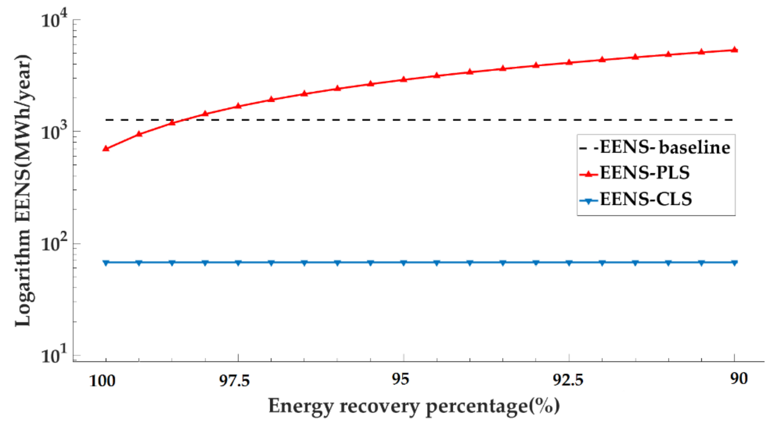
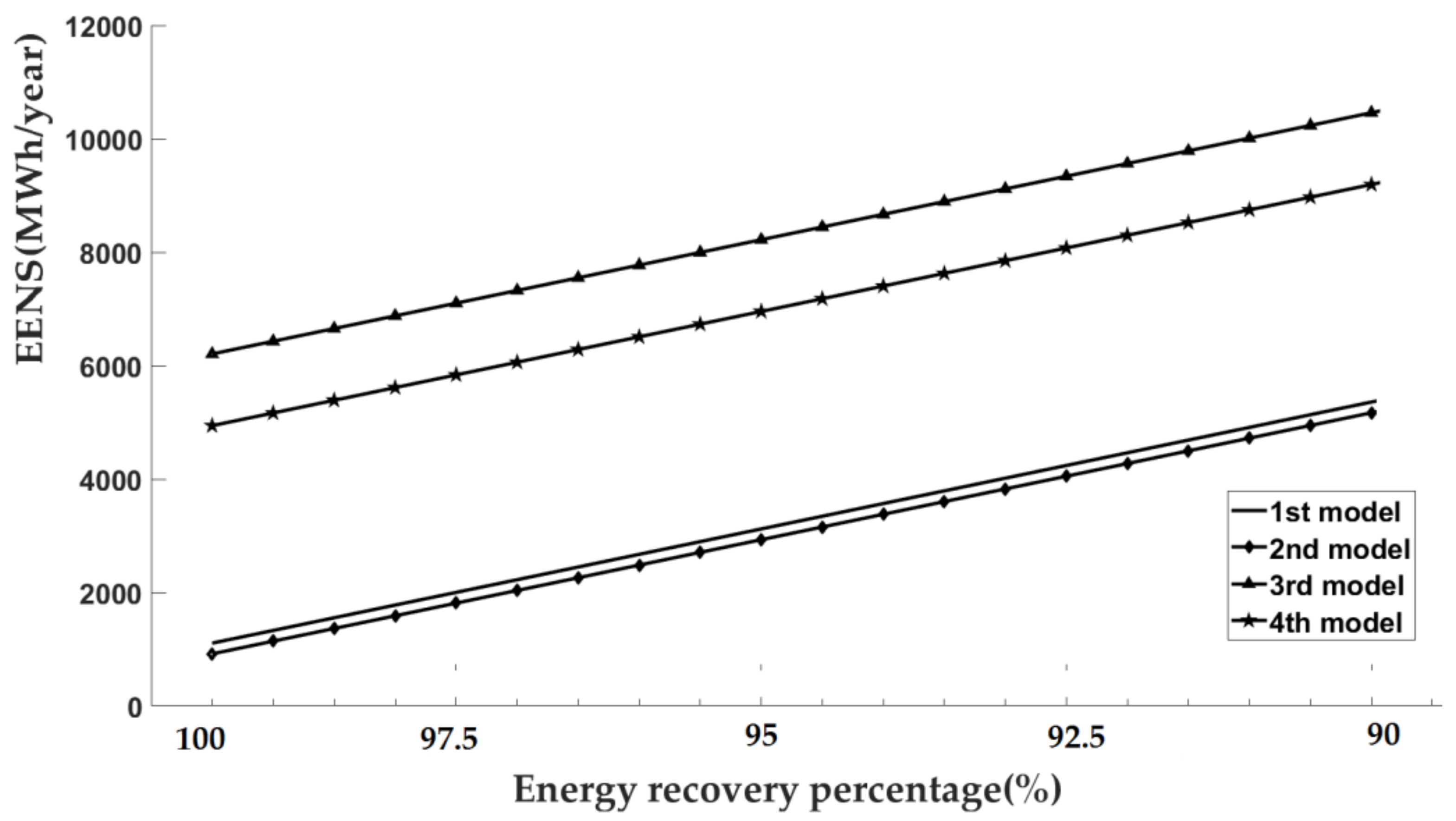
In Table 4, the percentage of energy recovery is assumed to be 100% all the time. Next, the variation of this percentage value towards the EENS is investigated and the results are given in Figure 10, Figure 11, Figure 12, Figure 13, Figure 14 and Figure 15. The percentage of energy recovery in these figures is reduced from 100% to 90% with step change of 0.5%. Logarithm scale of y-axis is used instead of the normal one as the EENS of CLS is considerably less than the PLS one. In PLS, load clipping is assumed constant (15% of peak load). In CLS, as there is no load clipping action, the energy curtailed due to the inadequacy of power supply is equivalent to the clipped energy in PLS. The baseline EENS value shown in all figures are from Case 1 (no load shifting program) to highlight specifically at which energy recovery percentage that the reliability enhancement benefit of PLS and CLS decay below the baseline EENS.
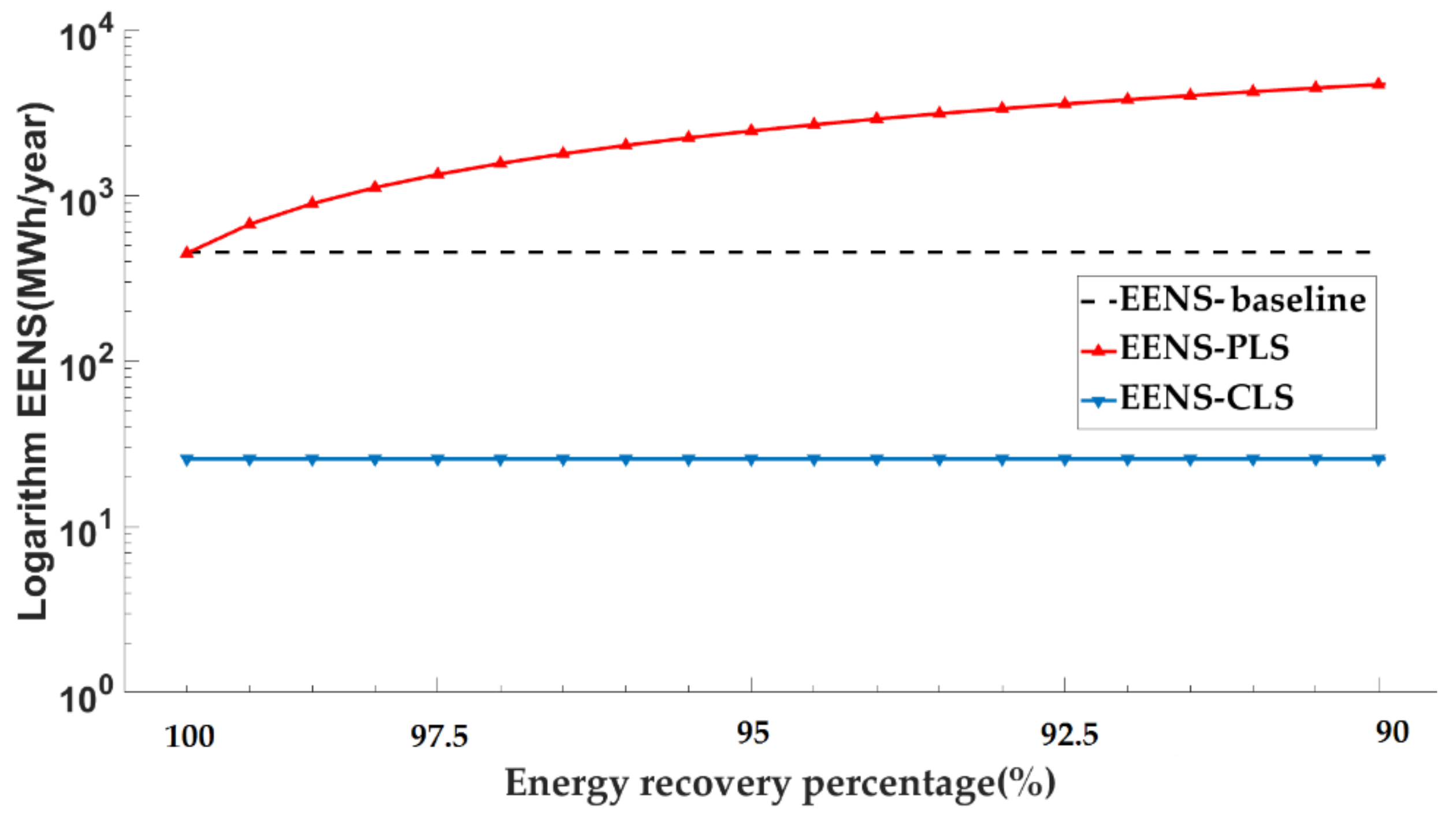
Figure 10 shows that, when the energy recovery percentage is below 99% (towards the right of x-axis) of clipped energy, the EENS of PLS exceeds the baseline value. In Figure 11, the EENS of PLS is worse and is always more than the baseline value. In both figures, the EENS of PLS increases as the energy recovery percentage decreases. In both PLS and CLS, the amount of unrecovered energy is due to the coincidence of small unused capacity of off-peak periods with large clipped load, as well as the variation on the energy recovery percentage. In addition, a portion of the EENS in PLS is also due to the inadequacy of power supply caused by random generator failures. These two figures show that the EENS of CLS is not affected by the variation of the energy recovery percentage. The reason for this is the CLS is implemented only when the power supply is unable to match the load demand and the amount of energy loss has been considered regardless of the percentage of energy recovery. In the PLS case, however, the entire load is clipped at the pre-specified peak load, contributing to more load that needs recovering all the time. For this reason, the effect due to the variation of the energy recovery percentage is more severe in PLS than CLS.
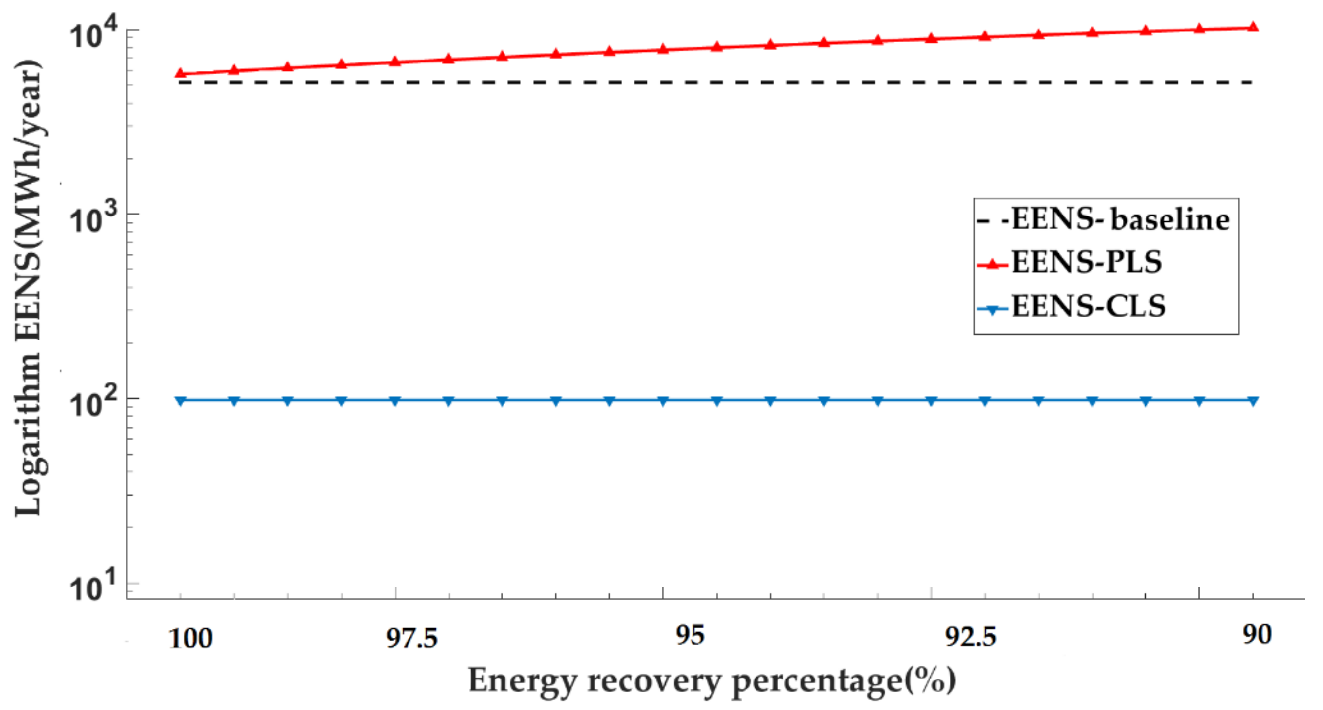
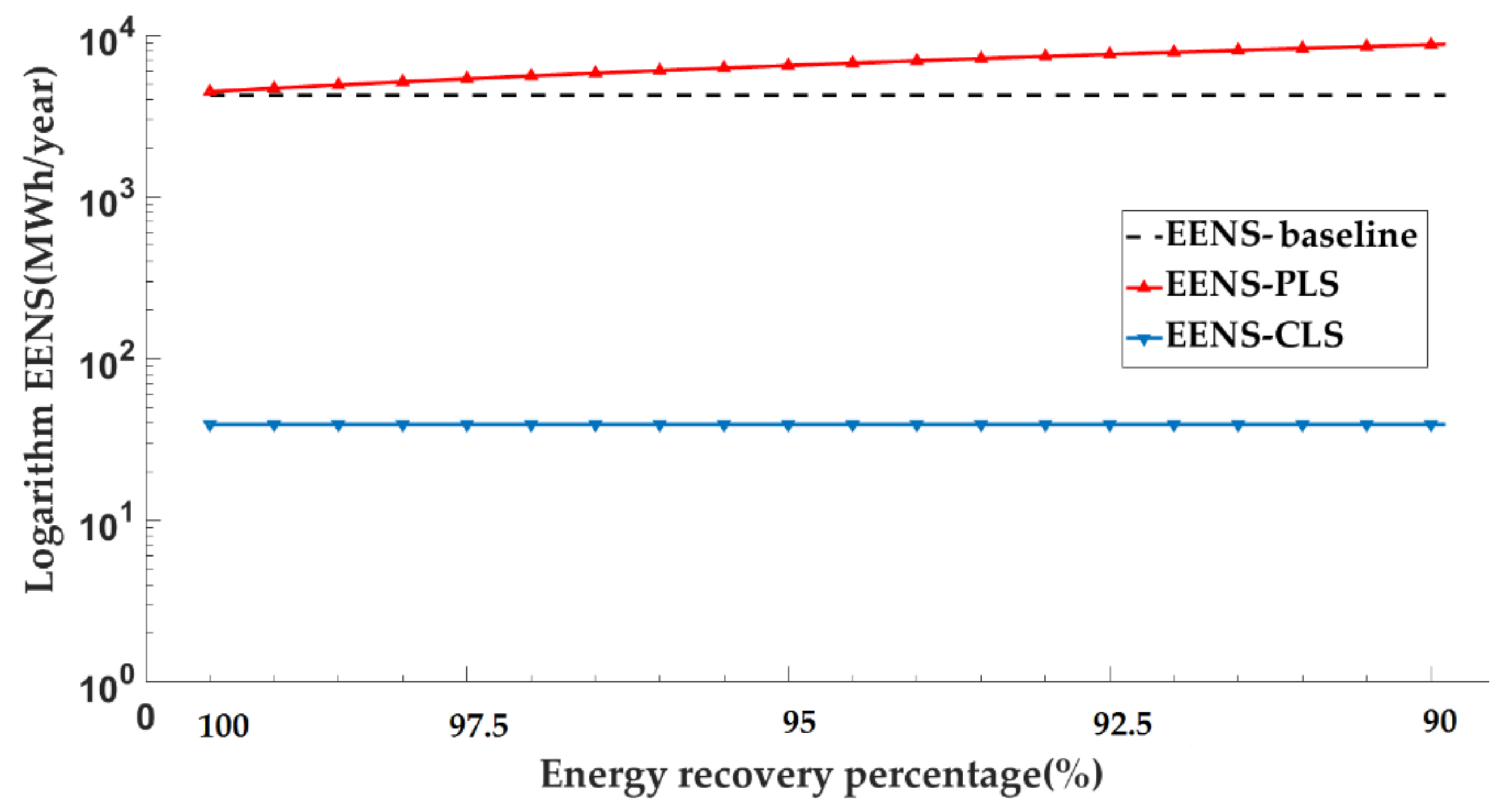
Similar observation can also be made for Figure 12 and Figure 13, where the Models 3 and 4 are implemented instead. When the energy recovery percentage is below 100% of clipped energy, almost all the EENS values of PLS are more than the baseline value. However, the EENS value of PLS are much higher than the first two models in Figure 10 and Figure 11. This is due to the planned maintenance and LFU considerations which increase the frequency and magnitude of energy curtailment.
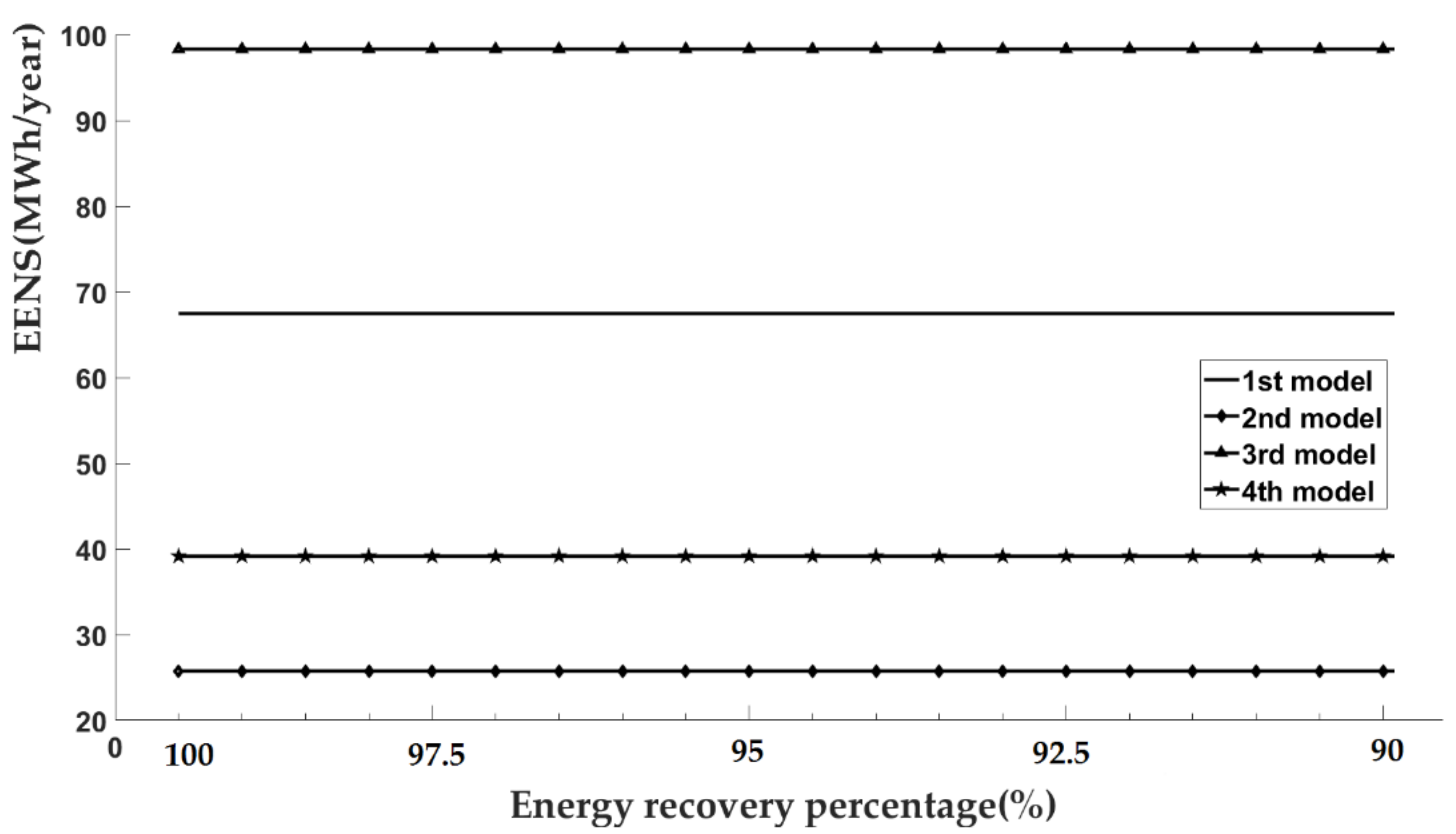
Figure 14 and Figure 15 consolidate the results from PLS and CLS from all the models, respectively, to better compare and illustrate the performance of each generator model as the energy recovery percentage decreases. Figure 14 shows that, when planned maintenance and LFU are considered (Models 3 and 4), the EENS values are always higher than when they are not (Models 1 and 2). The results also consistently show that generation systems with four-state model have lower EENS values than the two-state model, which represents a more realistic reliability assessment. Such trend is not available in Figure 15 as the CLS operation is more complex, where the curtailment and recovery of energy is based on when the power supply is inadequate. The inadequacy of power supply is further affected by the random failure of generators and the fluctuation of load demand over the entire period of a year. In CLS, EENS for all models remains constant as the energy recovery percentage decreases.
3.2. Discussion
- The results show that the EENS of PLS and CLS differs. The dynamic considerations of available system capacity and load in CLS have significant impacts towards the generation system adequacy and thus must be accurately modelled.
- The benefit of Load shifting depends on the ability of the system operator to recover clipped or curtailed load, which is affected by mismatch between the generation and load levels, the percentage limits of energy to be recovered, the willingness of consumers to participate in the load rescheduling program and the availability of the ancillary services that connect system operator with demand-side.
- During the inadequacy of power supply, most of the energy curtailed can be recovered in the same day. The unrecovered energy is due to the insufficient capacity of the off-peak period and this excess amount of energy is classified as the EENR in this paper.
- Power systems usually have reserve capacity margin to account for load uncertainty and generator outages as well as planned maintenance. The CLS program proposed in this paper is shown to be able to improve the adequacy of power supply without introducing additional power generating facility, presenting a viable alternative that is much cheaper and faster to be implemented.
- The above results show that CLS is clearly more effective than PLS in terms of improving the reliability of power supply. In CLS, optimal regulatory incentives can be determined by considering only the EENR instead of the entire clipped energy as in PLS. However, its benefit can only be realised if electricity suppliers are allowed to curtail and cycle load.
- The complexity of power systems couple with continuous load growth require applicable LFU and planned maintenance models to estimate future energy demands. Although this increases the EENS value, it provides a more realistic assessment. The results have shown that the application of the CLS program can overcome the unwanted reduction of the generation system. Thus, CLS is suitable in such considerations to mitigate the EENS deterioration. Moreover, the CLS program is also a more economic option as the system operators are able to add new generation facilities only after the load shifting program is unable to achieve the desired reliability level.
- In the four-state model, the duty cycle of peaking and cycling generation units are considered. These type of generation units, when compared to the based load unit, undergo more frequent start-up and shutdown but with lesser operating hours because they are only needed during peak periods, or when there is inadequate power supply. However, the frequently ramping generators burn more fuel and, therefore, incur more cost than if the generators are operating continuously. For this reason, peaking and cycling units are expensive to operate and should be minimised. The load shifting programs can help to achieve this by reducing the peak load levels, leading to the lesser needs of peaking and cycling units.
- As a whole, the load shifting programs investigated in this paper fit into the wider agenda of DSM. DSM programmes have received considerable attention in recent years due to their significant impacts on reliability. DSM programmes are expected to be implemented substantially in the next few decades to satisfy the requirements of new challenges, such as the intermittent nature of renewable energies, global environmental concerns and economic constraints. These programmes are significant, should be considered in the planning and operation phases of electrical power systems and must be integrated with generation-side management to maintain the reliability and increase the efficiency of power systems. The adequacy planning of generation systems has changed recently due to new trends and technologies, i.e., smart grids, advanced communication systems and the digital revolution. Power system planners currently have to consider various resources to satisfy the residential and industrial demand growth.
4. Conclusions
In this study, the impact of PLS and CLS on the adequacy of generation systems is investigated. Duty cycle and failure initiation of peaking and cycling generation units, planned maintenance and LFU are considered. A new CLS model that considers real-time fluctuation of load demand and generation availability is proposed and presented. The results presented in this paper indicate that, although the PLS program can improve the adequacy of the generation system, the CLS program provides greater reliability benefits. The reason for this is the CLS program only curtails load after the inadequacy of power supply is detected and is not performed indiscriminately throughout the entire load duration as in the PLS program. Hence, the CLS avoids the unnecessary degradation of the generation system reliability unlike PLS. The superiority of the CLS over the PLS is best illustrated in Figure 10, Figure 11, Figure 12 and Figure 13. In all figures, as the percentage of energy recovery is decreased, the CLS program manages to restrain the decay of the EENS index while the PLS cannot. From the results in Table 4, which has four models in all three cases, it is concluded that, when planned maintenance and LFU are considered (Models 3 and 4), the CLS program provides more reduction in the EENS value than the PLS program in the case without load shifting program. This again proves that the CLS program is a more robust load management technique than the PLS.
An additional observation to take note is that Models 3 and 4 significantly increase the EENS in all three cases as more generators are unavailable more often due to planned maintenance, and, at the same time, there is a possibility of encountering higher load levels than if LFU is not considered. This indicates that the assessment using planned maintenance and LFU is more realistic and is, therefore, more accurate, albeit the assessment of the EENS value of the generating system increases.
Finally, it is concluded that the models, algorithm and results presented in this paper provide valuable information and indicators for power system planners. In future studies, the production cost and environmental impacts of PLS and CLS programs, and the effect of uncertainty in load-shifting programs towards the reliability of power system can be considered.
Author Contributions
H.J.J., J.T. and H.H. conceived and designed the experiments; D.I. supervised the project; and J.T. and H.J.J. wrote the paper.
Acknowledgments
This work was partly supported by the USM short-term grant 304/PELECT/6031305, USM bridging grant 304.PELECT.6316117 and the UPE-USM grant 304/PELECT/6050385.
Conflicts of Interest
The authors declare no conflict of interest.
Nomenclature
| Pi | The probability of system state |
| Ci | The loss of load for system state |
| The number of simulation year | |
| The mean time to failure | |
| The mean time to repair | |
| The time to failure | |
| The time to repair | |
| Uniformly distributed random number between [0, 1] | |
| The failure rate | |
| The repair rate | |
| The average reserve shutdown time amongst periods of need, excluding scheduled outage | |
| The average in-need time per occasion of demand | |
| The starting failure probability of a generator | |
| The unit available capacity of the peaking and cycling generation unit | |
| The corresponding unit capacity | |
| A uniformly distributed random number between [0, 1] | |
| The original demand of the system | |
| , | The modified system load curves which result from implementing a load-shifting activity |
| The pre-specified peak demand | |
| The percentage of energy recovered amount, its range is | |
| The first time of the day when the original load is greater than the pre-specified peak (, | |
| The last time of the day when the original load is greater than the pre-specified peak | |
| , | The starting and ending times for the off-peak recovery of energy. |
| The duration of energy recovery, calculated as the difference between and | |
| The first modified load curve after subtracting from the original load | |
| The energy that must be shed during the period of adequacy deficiency. | |
| The second modified load curve after recovering energy to the first modified load curve | |
| The amount of added energy to each hour of recovery period | |
| The energy not recovered for each hour of energy recovery period | |
| The range of recovered energy, | |
| The first time during the day when the original load exceeds the system available capacity | |
| The last time during the day when the original load becomes equal or less than system capacity | |
| , | The starting and ending times for the off-peak recovery of energy |
| The instantaneous system available capacity | |
| Expected energy not supplied |
References
- Dehnavi, E.; Abdi, H. Determining optimal buses for implementing demand response as an effective congestion management method. IEEE Trans. Power Syst. 2017, 32, 1537–1544. [Google Scholar] [CrossRef]
- Allan, R. Reliability Evaluation of Power Systems; Springer Science & Business Media: Berlin, Germany, 2013. [Google Scholar]
- Li, W. Reliability Assessment of Electric Power Systems Using Monte Carlo Methods; Springer Science & Business Media: Berlin, Germany, 2013. [Google Scholar]
- Gellings, C.W. Evolving practice of demand-side management. J. Mod. Power Syst. Clean Energy 2017, 5, 1–9. [Google Scholar] [CrossRef]
- Gellings, C.W. The concept of demand-side management for electric utilities. Proc. IEEE 1985, 73, 1468–1470. [Google Scholar] [CrossRef]
- Gellings, C.W.; Chamberlin, J.H. Demand-Side Management: Concepts and Methods; The Fairmont Press Inc.: Lilburn, GA, USA, 1987. [Google Scholar]
- Gellings, C.W. Standars Corner IEEE PES Demand-Side Management Subcommittee. IEEE Power Eng. Rev. 1986, PER-6, 9–12. [Google Scholar]
- De Almeida, A.; Rosenfeld, A.H. Demand-Side Management and Electricity End-Use Efficiency 149; Springer Science & Business Media: Berlin, Germany, 2012. [Google Scholar]
- Teh, J.; Ooi, C.A.; Cheng, Y.-H.; Zainuri, M.A.A.M.; Lai, C.-M. Composite Reliability Evaluation of Load Demand Side Management and Dynamic Thermal Rating Systems. Energies 2018, 11, 466. [Google Scholar] [CrossRef]
- Patton, A.; Singh, C. Evaluation of load management effects using the OPCON generation reliability model. IEEE Trans. Power App. Syst. 1984, 11, 3229–3238. [Google Scholar] [CrossRef]
- Jabir, H.J.; Teh, J.; Ishak, D.; Abunima, H. Impacts of Demand-Side Management on Electrical Power Systems: A Review. Energies 2018, 11, 1050. [Google Scholar] [CrossRef]
- Huang, D.; Billinton, R. Effects of Load Sector Demand Side Management Applications in Generating Capacity Adequacy Assessment. IEEE Trans. Power Syst. 2012, 27, 335–343. [Google Scholar] [CrossRef]
- Sinsukprasert, P. Effects of Demand Side Management on Power System Reliability: A Case Study of Thailand, 1998. Available online: https://repository.upenn.edu/dissertations/AAI9829992 (accessed on 6 July 2018).
- Malik, A.S. Simulation of DSM resources as generating units in probabilistic production costing framework. IEEE Trans. Power Syst. 1998, 13, 1528–1533. [Google Scholar] [CrossRef]
- Malik, A. Modelling and economic analysis of DSM programs in generation planning. Int. J. Electr. Power Energy Syst. 2001, 23, 413–419. [Google Scholar] [CrossRef]
- Narimani, M.R.; Nauert, P.J.; Joo, J.Y.; Crow, M.L. Reliability assesment of power system at the presence of demand side management. In Proceedings of the IEEE Power and Energy Conference at Illinois (PECI), Champaign, IL, USA, 19–20 February 2016; pp. 1–5. [Google Scholar]
- Malik, A.S. Dynamic generating costs in DSM planning. Energy 1999, 24, 1–8. [Google Scholar] [CrossRef]
- Tanrioven, M.; Alam, M. Impact of load management on reliability assessment of grid independent PEM fuel cell power plants. J. Power Sources 2006, 157, 401–410. [Google Scholar] [CrossRef]
- Karunanithi, K.; Saravanan, S.; Prabakar, B.; Kannan, S.; Thangaraj, C. Integration of Demand and Supply Side Management strategies in Generation Expansion Planning. Renew. Sustain. Energy Rev. 2017, 73, 966–982. [Google Scholar] [CrossRef]
- Diewvilai, R.; Nidhiritdhikrai, R.; Eua-arporn, B. Demand side management worth evaluation under generation system planning framework. In Proceedings of the 2012 9th International Conference on Electrical Engineering/Electronics, Computer, Telecommunications and Information Technology (ECTI-CON), Phetchaburi, Thailand, 16–18 May 2012; pp. 1–4. [Google Scholar]
- Salehfar, H.; Patton, A. Modeling and evaluation of the system reliability effects of direct load control. IEEE Trans. Power Syst. 1989, 4, 1024–1030. [Google Scholar] [CrossRef]
- Ahsan, Q. Load management: Impacts on the reliability and production costs of interconnected systems. Int. J. Electr. Power Energy Syst. 1990, 12, 257–262. [Google Scholar] [CrossRef]
- Billinton, R.; Lakhanpal, D. Impacts of demand-side management on reliability cost/reliability worth analysis. IEE Proc. Gener. Transm. Distrib. 1996, 143, 225–231. [Google Scholar] [CrossRef]
- Calsetta, A.; Albrecht, P.; Cook, V.; Ringlee, R.; Whooley, J. A four-state model for estimate of outage risk for units in peaking service. IEEE Trans. Power App. Syst. 1972, 618–627. [Google Scholar] [CrossRef]
- Allan, R.N.; Billinton, R.; Abdel-Gawad, N. The IEEE reliability test system-extensions to and evaluation of the generating system. IEEE Trans. Power Syst. 1986, 1, 1–7. [Google Scholar] [CrossRef]
- Billinton, R.; El-Sheikhi, F.A. Preventive maintenance scheduling in power generation systems using a quantitative risk criterion. Can. Electr. Eng. J. 1983, 8, 28–39. [Google Scholar] [CrossRef]
- Limaye, D. Implementation of demand-side management programs. Proc. IEEE 1985, 73, 1503–1512. [Google Scholar] [CrossRef]
- Abaravicius, J. Demand Side Activities for Electric Load Reduction. Ph.D. Thesis, Lund University, Lund, Sweden, 2007. [Google Scholar]
- Billinton, R.; Huang, D. Effects of load forecast uncertainty on bulk electric system reliability evaluation. IEEE Trans. Power Syst. 2008, 23, 418–425. [Google Scholar] [CrossRef]
- El-Sheikhi, F.A.; Billinton, R. Load forecast uncertainty consideration in generating unit preventive maintenance scheduling for single systems. In Proceedings of the Third International Conference on Probabilistic Methods Applied to Electric Power Systems, London, UK, 3–5 July 1991; pp. 241–245. [Google Scholar]
- Zhai, D.; Breipohl, A.; Lee, F.; Adapa, R. The effect of load uncertainty on unit commitment risk. IEEE Trans. Power Syst. 1994, 9, 510–517. [Google Scholar] [CrossRef]
- Subcommittee, P.M. IEEE Reliability Test System. IEEE Trans. Power App. Syst. 1979, 98, 2047–2054. [Google Scholar] [CrossRef]
Figure 1.
Hierarchical zones.

Figure 2.
HLI model.

Figure 3.
Two-state model for a base load unit.

Figure 4.
Four-state model for peaking and cycling load units.

Figure 5.
Various DSM techniques.

Figure 6.
ENR due to peak-clipping actions for PLS.

Figure 7.
ENR due to load curtailment action for CLS.

Figure 8.
Seven-step approximation of the normal distribution.

Figure 9.
Flow chart of PLS and CLS.

Figure 10.
EENS of PLS and CLS for Model 1.

Figure 11.
EENS of PLS and CLS for Model 2.

Figure 12.
EENS of PLS and CLS for Model 3.

Figure 13.
EENS of PLS and CLS for Model 4.

Figure 14.
EENS of PLS for all models.

Figure 15.
EENS of CLS for all models.


Table 1.
Planned maintenance schedule for each generation unit capacity.
| Capacity (MW) | Scheduled Maintenance (Weeks/Year) | Outage Schedule (Number in Bracket Is Week) |
|---|---|---|
| 2 × 400 | 6 | (10–15) and (35–40) |
| 1 × 350 | 5 | (31–35) |
| 3 × 197 | 4 | (8–11), (15–18) and (40–43) |
| 4 × 155 | 4 | (6–9), (12–15), (26–29) and (36–39) |
| 3 × 100 | 3 | (20–22), (27–29) and (41–43) |
| 4 × 76 | 3 | (3–5), (15–17), (30–32) and (34–36) |
| 6 × 50 | 2 | (16–17), (21–22), (27–28), (31–32), (38–39) and (41–42) |
| 4 × 20 | 2 | (9–10), (12–13), (12,13) and (33–34) |
| 5 × 12 | 2 | (9–10), (26–27), (33–34), (38–39) and (41–42) |
No maintenance is scheduled on Weeks 1, 2, 19, 23–25 and 44–52 due to the high load level in these periods.
Table 2.
Reliability indices incorporating LFU.
| Std. Deviations from Mean | Load Level (MW) | Reliability Index | Probability | Weighted |
|---|---|---|---|---|
| −3 | 2850 − (15% × 2850) = 2422.5 | a | 0.006 | a × 0.06 |
| −2 | 2850 − (10% × 2850) = 2565.0 | b | 0.061 | b × 0.61 |
| −1 | 2850 − (5% × 2850) = 2707.5 | c | 0.242 | c × 0.242 |
| 0 | 2850 − (0% × 2850) = 2850.0 | d | 0.382 | d × 0.382 |
| +1 | 2850 + (5% × 2850) = 2992.5 | e | 0.242 | e × 0.242 |
| +2 | 2850 + (10% × 2850) = 3135.0 | f | 0.061 | f × 0.061 |
| +3 | 2850 + (15% × 2850) = 3277.5 | g | 0.006 | g × 0.006 |
| Reliability index = Σ weighted of reliability index = a × 0.06 + b × 0.61 + c × 0.242 + d × 0.382 + e × 0.242 + f × 0.061 + g × 0.006 | ||||
Table 3.
The priority order and expected energy production of the IEEE-RTS generation system.
| Priority Order | Capacity (MW) | Unit Type | Expected Energy Production (GWh) | Load Supplied |
|---|---|---|---|---|
| 1–6 | 50 × 6 | Hydro | 2594.592 | Base |
| 7–8 | 400 × 2 | Nuclear | 6142.754 | |
| 9 | 350 × 1 | Coal | 2521.737 | |
| 10–12 | 197 × 3 | Oil | 3002.401 | |
| 13–16 | 155 × 4 | Coal | 680.454 | |
| 17–19 | 100 × 3 | Oil | 333.287 | Cycling |
| 20–23 | 76 × 4 | Coal | 18.638 | |
| 24–28 | 12 × 5 | Oil | 1.149 | Peaking |
| 29–32 | 20 × 5 | Oil | 0.885 |
Table 4.
Proposed models of PLS and CLS.
| Model No. | EENS MW h/year | ||
|---|---|---|---|
| 1st Case: No Load Shifting | 2nd Case: PLS | 3rd Case: CLS | |
| Model 1: 2-state for all units | 1144.6422 | 898.9592 | 68.9158 |
| Model 2: 4-state for peaking and cycling units | 869.7892 | 822.5749 | 25.7486 |
| Model 3: Model 1 + LFU & maintenance | 6235.3378 | 6258.9655 | 98.3171 |
| Model 4: Model 2 + LFU & maintenance | 5208.4484 | 4607.0723 | 39.1608 |
© 2018 by the authors. Licensee MDPI, Basel, Switzerland. This article is an open access article distributed under the terms and conditions of the Creative Commons Attribution (CC BY) license (http://creativecommons.org/licenses/by/4.0/).
Share and Cite
MDPI and ACS Style
Jabir, H.J.; Teh, J.; Ishak, D.; Abunima, H. Impact of Demand-Side Management on the Reliability of Generation Systems. Energies 2018, 11, 2155. https://doi.org/10.3390/en11082155
AMA Style
Jabir HJ, Teh J, Ishak D, Abunima H. Impact of Demand-Side Management on the Reliability of Generation Systems. Energies. 2018; 11(8):2155. https://doi.org/10.3390/en11082155
Chicago/Turabian StyleJabir, Hussein Jumma, Jiashen Teh, Dahaman Ishak, and Hamza Abunima. 2018. "Impact of Demand-Side Management on the Reliability of Generation Systems" Energies 11, no. 8: 2155. https://doi.org/10.3390/en11082155
Note that from the first issue of 2016, this journal uses article numbers instead of page numbers. See further details here.