Two-Level Evolutionary Multi-objective Optimization of a District Heating System with Distributed Cogeneration

Abstract

The paper deals with the modeling and optimization of an integrated multi-component energy system. On-off operation and presence-absence of components must be described by means of binary decision variables, besides equality and inequality constraints; furthermore, the synthesis and the operation of the energy system should be optimized at the same time. In this paper a hierarchical optimization strategy is used, adopting a genetic algorithm in the higher optimization level, to choose the main binary decision variables, whilst a MILP algorithm is used in the lower level, to choose the optimal operation of the system and to supply the merit function to the genetic algorithm. The method is then applied to a distributed generation system, which has to be designed for a set of users located in the center of a small town in the North-East of Italy. The results show the advantage of distributed cogeneration, when the optimal synthesis and operation of the whole system are adopted, and significant reduction in the computing time by using the proposed two-level optimization procedure.

1. Introduction

A more thorough integration among energy systems is expected to significantly contribute to reducing primary energy consumption, as well as global pollutant emissions and energy costs for final users. Integrated district heating networks (DHN) and combined heat and power (CHP) are of particular interest for the object of defining an efficient system for distributed energy generation and are widely discussed in the literature, i.e., in terms of role and opportunities in a country like Denmark [1], United Kingdom [2] and Italy [3,4] or considering a review of the different technology opportunities [5] and of the energy sources [6] also for combined heat, cooling and power systems (CHCP). The expected advantages of energy integration can, in fact, be obtained in real world applications only if the structure (synthesis) and the management of the whole system are carefully optimized. For instance, in [7] a computational framework is proposed to face the problem at city districts level, in [8] a mixed integer linear programming (MILP) model is used to determine the type, number and capacity of equipment in CHCP systems installed in a tertiary sector building, in [9] a modelling and optimization method is developed for planning and operating a CHP-DH system with a solar thermal plant and a thermal energy storage, in [10] a detailed optimization model is presented for planning the short-term operation of combined cooling, heat and power (CCHP) energy systems, for a single user in [11] an algorithm for the minimization of a suitable cost function is applied to optimize CHP commercial and domestic systems with variable heat demand.

The design optimization of integrated multi-component energy systems has to be performed making reference to the optimal operation for each design alternative; this generally require a binary variable set to be introduced to describe both the existence/absence and the on/off operation status of components and energy network lines inside the model. Besides these, other continuous variables have to be introduced for modelling the energy and material flows exchanged among components, as well as other possible design options [8,12,13].

In addition to this complex variable set, the variation of the thermal demands of the final users has also to be taken into account. Thus, a mixed integer non linear programming (MINLP) problem has generally to be solved for obtaining the optimal synthesis and operation of the integrated system, with a high computational effort. A general introduction to MILP, MINLP and other possible approaches to the design and synthesis optimization of energy systems can be found in [14]. Recently, the MINLP approach has been used, for instance in [15,16] to optimize the CCHP systems of different buildings with solar energy integration.

The computational effort can be reduced if the whole problem is faced by defining two (or more) levels, which can be solved dealing with a reduced number of independent variables [17], or if it is decomposed into many sub-problems, which have to be solved with an iterative procedure [18,19,20]. In both cases the solution could be more easily obtained if the problem were described with sufficient precision by means of a linear model (MILP), even if additional variables are introduced for considering strong non-linear relations among flows of both energy and mass [12,13].

Unfortunately, when there is a high number of binary variables present in almost all sub-problems, the coupling variables, which allow each sub-problem to be solved consistently with the optimal solution of the whole system [21,22,23], become too changeable to allow the convergence of the optimization process toward the actual optimum.

In the present paper, such difficulties are overcome by using a novel approach, characterized by a two-level hierarchical optimization strategy which does not require an explicit system decomposition. In the proposed method a genetic algorithm is used in the higher optimization level, to choose the main binary decision variables, whilst a MILP algorithm is used in the lower level, to choose the optimal operation of the system and to supply the merit function to the genetic algorithm.

The proposed system model is intended for district-level implementation and is concerned with the optimal layout and operation of CHP units, deployed in different buildings, as well as with the optimal configuration of one, or more micro-district heating grids. A central CHP plant, besides a set of micro-CHP gas turbines distributed among the involved buildings, along with the installation of thermal collectors and photovoltaic (PV) panels have been considered to further improve the energy efficiency and sustainability of the whole system.

The main optimization was aimed at minimizing the total annual cost for owning, maintaining and operating of the whole system. Furthermore, the optimal solution, beside satisfying the electric energy and heating demands of each building throughout the year, should allow a minimum environmental impact. Therefore, a multi-objective optimization has been performed, by considering, as a second objective of the optimization, the avoided CO₂ compared to the conventional energy supply.

In summary, the method allows the identification of the optimal configuration of the micro-district heating grids, of the design of the CHP units in each building and the optimal operation of the whole energy system inside a unique optimization procedure, satisfying the energy demands of multiple users.

The focus of this paper is mainly on the performance of the hierarchical optimization algorithm and on the option of easily performing a multi-objective optimization, by using the numerical solution of an exemplifying case study. The expectation is that the developed optimization strategy highlights a reduction in the computing time compared with the direct implementation of the whole problem in a single level MILP solver. Therefore, the presented method could be applied to distributed cogeneration systems with a number of energy users and district heating branches much higher than those considered in the case study.

2. Model of a Cogeneration System with District Heating

In the following, a distributed cogeneration and district heating system is considered, whose model includes both a set of micro-cogeneration gas turbines (TG), a centralized cogeneration system based on an internal combustion engine (ICE), photovoltaic panels (PV), solar thermal collectors (ST) and district heating grid that can connect the users by means of different layouts. The model of a similar energy system has been used to discuss a different issue (the effect of different economic support policies on the economic operation of the system) in a couple of previous paper of the same authors [24,25]. The simultaneous optimization of both the configuration and the operation of distributed cogeneration plants is, in a mathematical sense, a non-linear problem (because of the non-linearity of the interconnection among the relations that express the partial-load behavior of each engine. To reduce the complexity of the problem, it is convenient though to assume the existence of a discrete number of intervals on which these relations are well approximated by a linear form (see, for instance, [26,27] and [25,28] for a single, or multiple energy user, respectively). In this way, a MILP problem is obtained.

Notice that, in the discretized problem, each time interval is solved as the power and heat demand of each building were constant, therefore neglecting also the effect of dynamic load variation on the performance of the energy supplying components, but considering only their performance evaluated at different level of constant load. In other words, the dynamic response of engine and microturbines are considered much faster than the dynamic variations in the demand of the users. Notice also that this does not mean that each time interval could be optimized individually, because of the decision variables describing the existence/absence of components and connections inside the model, which link together all time intervals. In this work, discrete time intervals of one hour have been considered.

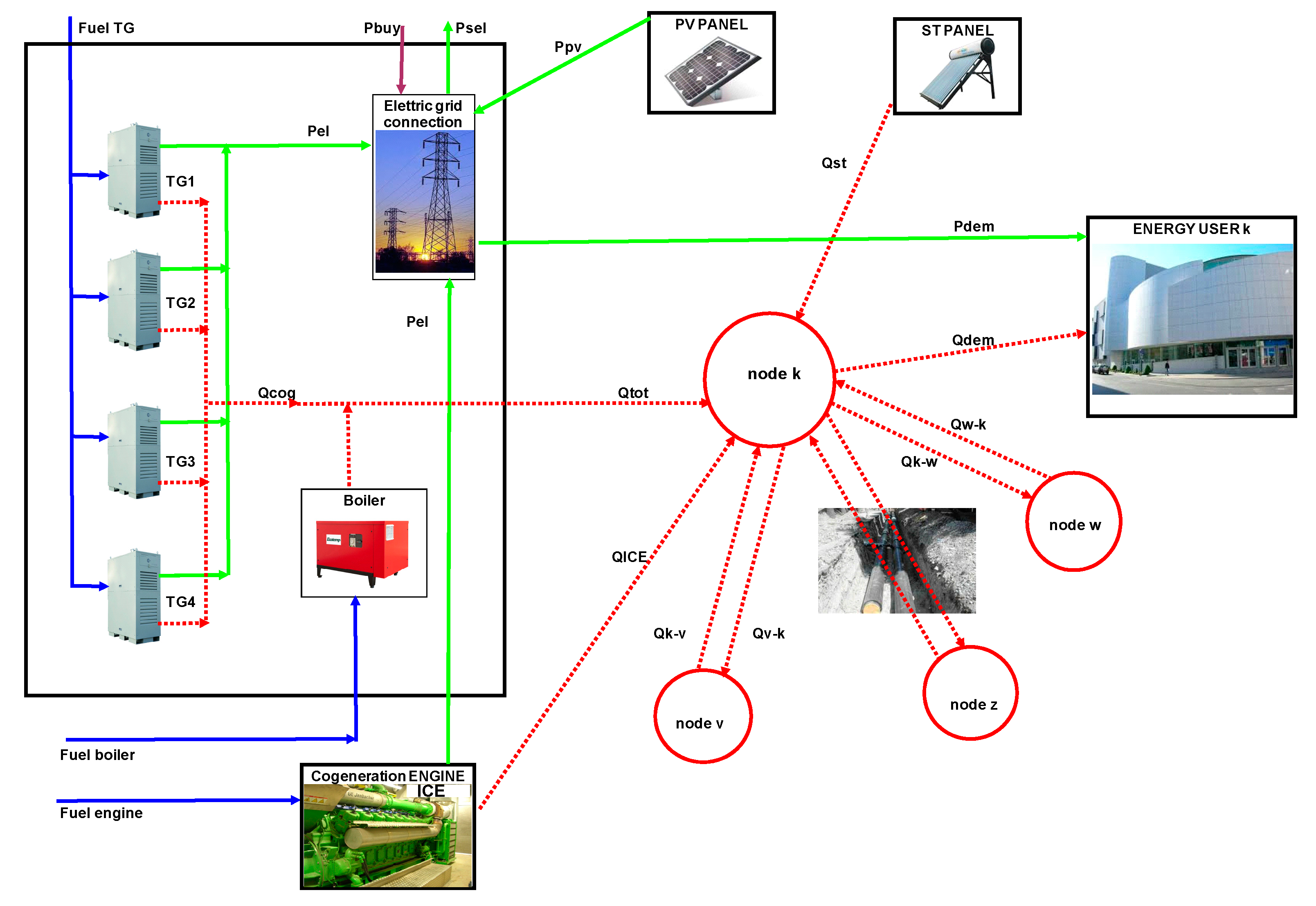
The distributed cogeneration and district heating system is schematized in Figure 1, where the generic user k is shown, which receives the thermal energy from the corresponding node k of the network. The latter receives the thermal energy from the cogeneration units, from the solar thermal collectors and from the Boiler possibly present at the same user k, but is also able to exchange thermal energy with the other nodes of the network (in Figure 1 there are shown three other generic nodes: v, w, z). Likewise, electrical energy arrives to the user through an electric connection where the electrical energy, eventually produced by cogenerators and PV panels installed at the node, can be integrated or exchanged with the external electrical network. Therefore, the problem cannot be solved separately for each cogeneration unit installed at a specific building because each of them is connected with the district heating network through a node where income and outcome thermal energy flows can be potentially exchanged with any other node of the network and the heat demand faced by each unit is not defined “in advance”. Then, the optimal operation has to be defined jointly with the optimal synthesis of the district heating micro-grids and with the number and position of CHP engines.

In each time interval, the energy system is described by means of the amount of every exchanged energy flow and by two sets of binary optimization variables expressing the existence/not-existence of the components and their on/off operation. Other design binary variables and continuous operating variables can also be used to describe the district heating network to be optimized, without violating the model linearity. In the following, the equations of the MILP model used in the presented optimization procedure are summarized.

In Equation (1) the total annual cost for owning, maintaining and operating the whole system is shown. This variable has been assumed as the objective function of the optimization procedure. In detail, the operating costs are obtained by adding the cost for the purchase of all the external fuel energy flows and subtracting the incomes for the electric energy possibly sold to another grid, during the whole year, while the owning costs are simply obtained by multiplying the total capital cost of each kind of component by the corresponding capital cost recovery factor, and the maintaining costs are regarded as proportional to the electric energy produced all the yearlong.

Variables X (j, k) represent the existence/not-existence of CHP engine (TG or ICE) “j” inside building “k”, while variables y (i, j, k) ≤ X(j, k) represent the on/off operation of the same CHP engine at the time interval “i”. Analogously, the existence/not-existence into the district heating network of a pipeline connecting node “v” with node “k” is expressed by variables r (k, v). The thermal power, flowing from node “v” to node “k” during the time interval “i” is expressed by variables Q (i, k, v), while D_HN (k, v) is the maximum heat flow in that pipeline, in all time interval of the whole year (Figure 1):

cost_TOT = Σ Fuel_CHP (i, j, k) ∗ C_FuelCHP (i) + Σ [Fuel_boil (i, k) ∗ C_Fuelboil (i) + Pbuy (i, k) ∗ C_BUY (i, k)
− Psel (i, k) ∗ C_SEL (i)] + fa_CHP ∗ cost_CHP + fa_HN ∗ cost_HN + fa_PV ∗ cost_PV + fa_ST ∗ cost_ST + cost_man

(1)

where:

cost_PV = Σ C_PV ∗ A_PV (k)

(2)

is the total capital cost of PV panels

cost_ST = Σ C_ST ∗ A_ST (k)

(3)

is the total capital cost of ST collectors

cost_CHP = Σ C_CHP (j, k) ∗ X (j, k)

(4)

is the total capital cost of CHP components

cost_HN = Σ [D_HN (k, v) ∗ E + r (k, v) ∗ F] ∗ l (k, v)

(5)

is the total capital cost of the district heating networks

cost_man = Σ C_man ∗ Pel (i, j, k)

(6)

is the maintenance cost of the whole system.

The cost of each pipeline (branch) per unit length, can be considered as a linear function of the maximum nominal heat flow of the same pipeline [25], whilst the efficiency of the integration boilers can be regarded as a constant.

Note that the existence of TG, ICE and branches of the DHN are described by (binary) decision variables whilst the extensions of PV and ST panel surfaces (A_PV and A_ST, respectively) are continuous decision variables, but none of them depend on the specific time interval. On the contrary, the on/off operation of the same components and the thermal and electrical energy flows, exchanged inside the system, are also decision variables (binary and continuous, respectively) but they can change by switching from one time interval to the next one. A first set of constraints represents the performance maps of the components which have been linearized, with negligible approximation:

Fuel_CHP (i, j, k) = A (j, k) ∗ Pel (i, j, k) + B (j, k) ∗ y (i, j, k)

(7)

Qcog (i, j, k) = M (j, k) ∗ Pel (i, j, k) + N (j, k) ∗ y (i, j, k)

(8)

P_min (j, k) ∗ y (i, j, k) ≤ Pel (i, j, k) ≤ P_max (j, k) ∗ y (i, j, k)

(9)

In this paper, the coefficients of the linearized performance maps of the components have been regarded as time dependent, because they are affected by temperature variations.

In addition, the maximum nominal heat flow and the heat flow direction of each pipeline has to be respected:

D_HN (k, v) ≥ Q (i, k, v) ≥ 0

(10)

D_HNmin (k, v) ∗ r (k, v) ≤ D_HN (k, v) ≤ D_HNmax (k, v) ∗ r (k, v)

(11)

r (k, v) + r (v, k) ≤ 1

(12)

Additional constraints state that both electrical and thermal demands have to be satisfied in all time intervals. In details, the cogeneration microturbines, the ICE, the auxiliary boilers and the solar collectors have to satisfy the thermal demand, while the same cogeneration microturbines and ICE have to satisfy the electrical demand jointly with the PV panels and the external purchase of electricity:

Qint (i, k) = Qdem (i, k) − Σ Qcog (i, j, k) + Qdiss (i, k) + Σ Q (i, k, v) − Σ Q (i, v, k) ∗ (1 − d (v, k)) − Q_ST (i, k)

(13)

Psel (I, k) = Σ Pel (i, j, k) − Pdem (i, k) + Pbuy (i, k) + P_PV(i, k)

(14)

A simplified model is used for the district heating network, in order of allowing a linear formulation of the optimization problem and reducing the computational effort. In detail, each pipeline is regarded as made up by two collectors: a delivery collector and a return one. Thermal losses along the district heating network generally depend on both the heat flow Q and the pipeline length, in this model they have been taken into account through a constant factor δ, expressing the fraction of Q that is expected to be lost, per unit length:

d (v, k) = (δ/100) ∗ l (v, k)

(15)

The mass flow rates in the DHN pipelines are not explicitly calculated in the model, but only heat flows are taken into account in the linear optimization. These mass flow rates can be easily obtained for the optimal solutions by introducing the proper values of the delivery and return temperatures, consistent with the thermal users considered. The energy consumed by the circulation pumps of the DHN is regarded as negligible, with respect to the electrical demand of the users, therefore it is not considered in the electric energy balance.

The energy efficiency of both solar thermal and photovoltaic panels can be regarded as linear vs. the temperature difference between the fluid collector average temperature and the outside ambient [29,30]:

η_ST = −7.5 (t − t°)/G + 0.7

(16)

η_PV = −0.0009 (t° − t) + 0.1987

(17)

where t is the fluid collector average temperature, t° is the ambient temperature and G [W/m²] is the solar radiation. The numerical coefficients of the linear regression of η_ST in Equation (16) are expressed in [W/°Cm²] according to the indications of [29], while the numerical coefficients of the linear regression of η_PV in the Equation (17) are expressed in [1/°C] according to the indications of [31]. These coefficients refer to collectors having an inclination equal to 30° with respect to the ground, placed in a site close to the town of the following case study, and south oriented. They exhibit an average energy efficiency equal to about 42%, by using the data for G and t° presented in [25].

The CO₂ emissions as a result of the operation of the whole CHP and DHN can be calculated by introducing the carbon intensity (CI) of fuels and purchased/sold electricity to the grid. Then, the avoided CO₂ emissions can be easily calculated as the difference between the conventional and the CHP and DHN energy production, to supply the same users.

3. Case Study

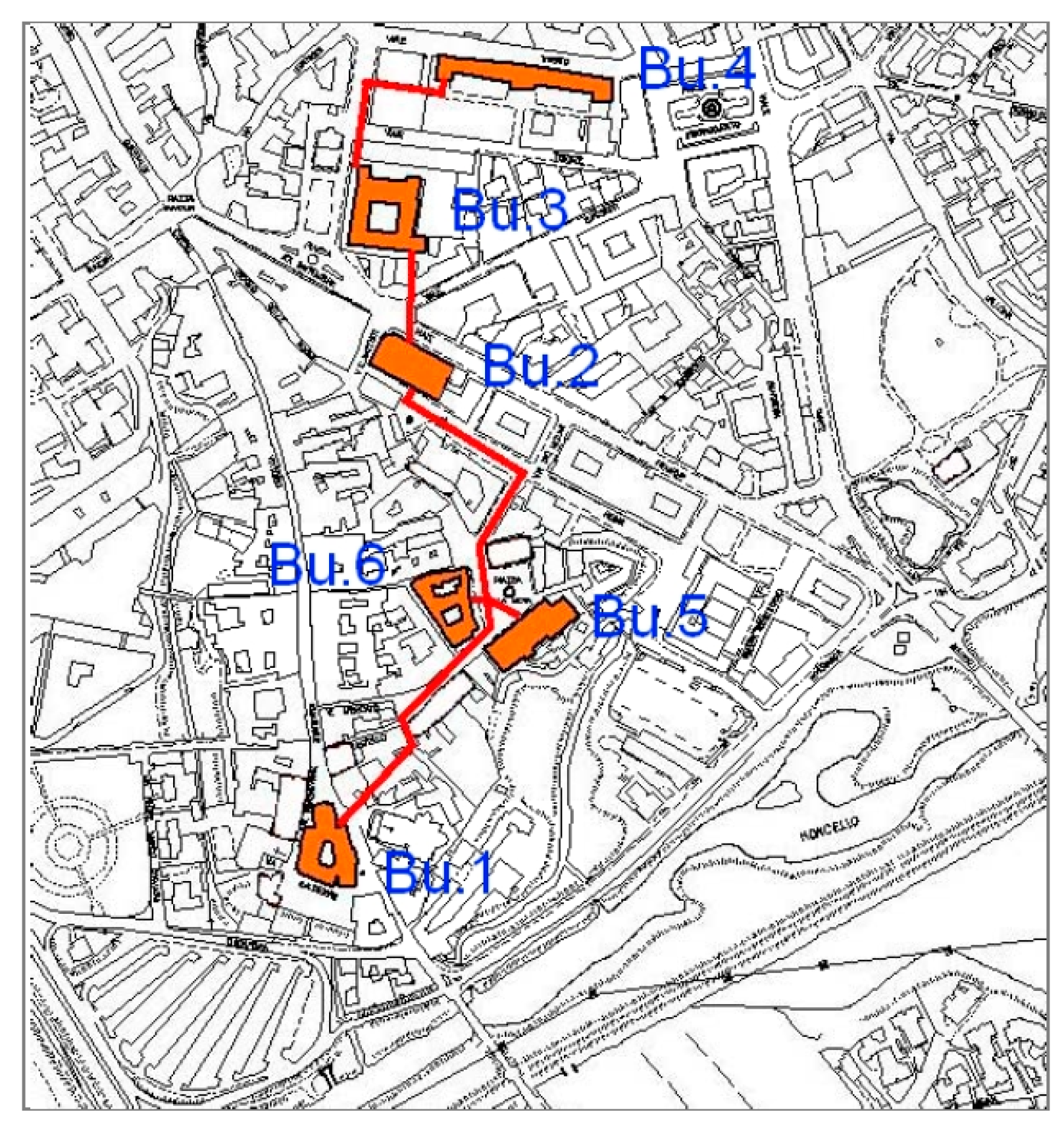
The optimization model has been applied to a distributed cogeneration system with district heating, taking as a reference for the supplying of thermal energy and electricity the consumptions of six public buildings in the center of the city of Pordenone (Italy) [32] considering this as representative of generic commercial building systems [33].

The conventional power supply, for the six buildings considered, involves an annual cost of 796,064 €/year, for the purchase of 2959 MWh of electrical energy and for the production of 4846 MWh of thermal energy by conventional boilers, fed with natural gas [24].

In Figure 2 it is shown the city center map with the location of the six buildings and a possible pipeline network of the district heating system. To reduce the overall number of variables, the whole year can be modeled by taking into account a small number of “typical days” for energy demand and rates. In the case study, 24 typical days have been considered (one working day and one public holiday, for each month). In this way the energy demand of the whole year is adequately approximated by repeating a proper number of times each typical day. This approach is widely accepted in literature (see, for instance, [15,16,34]). Recently, Pfenninger presented a systematic analysis of the different techniques to reduce the computational effort for energy models resolution [35], including time slices and typical days or weeks identification.

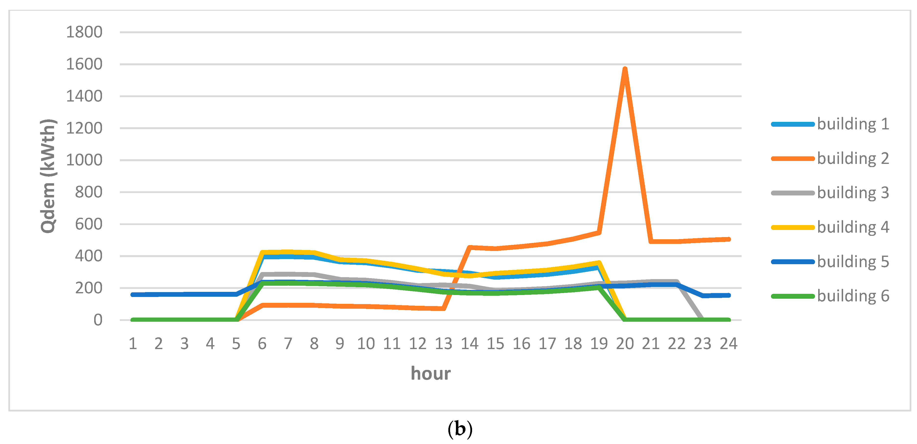
In [36] the approach of identifying a set of proper typical days is used in the optimal design of a multi-energy system with seasonal thermal storage, while in [37] an improved adaptive genetic algorithm is proposed to model the typical day load sequence for multi-objective optimization of a distributed generation system. In Figure 3a,b, the energy demands of the six buildings are shown for a winter working day, as an example. It can be noticed that the thermal demand peak of building 2 in an evening hour, is caused by the specific activity of a city theatre, that starts in the evening requiring the heating of a big empty volume. 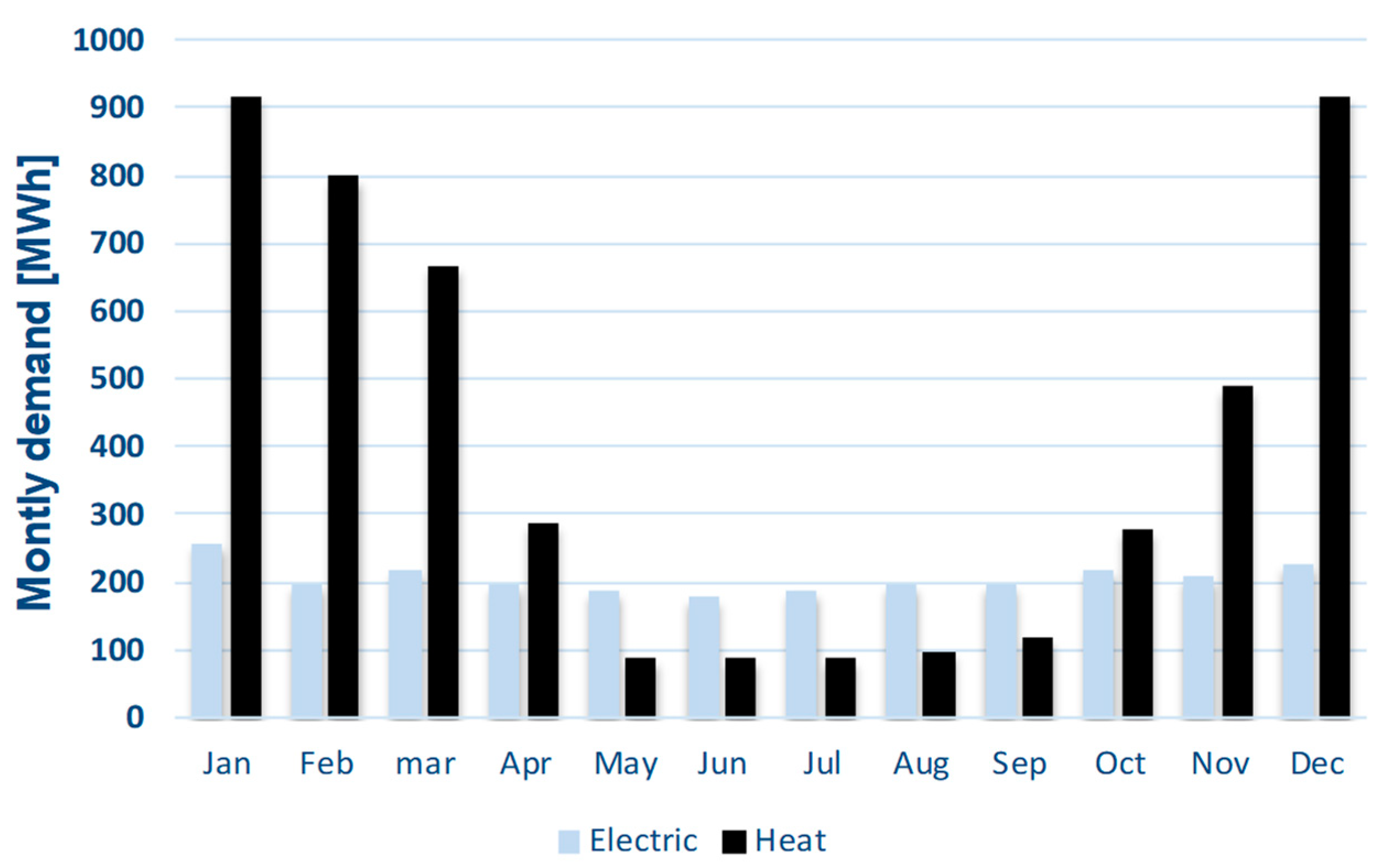In Figure 4 the total monthly energy demands are shown for all the year. Notice that the thermal demand shows strong seasonal variations, as it is common for civil buildings in the central European region. During summer time, the usage of the buildings is less frequent, so that the electrical demand is lower than in the winter time, while the opposite often occurs today for dwelling buildings, because of the air conditioning consumptions.

In each building a local cogeneration unit may be installed, with a maximum number of microturbines equal to 4, jointly with an integration boiler; all buildings are also connected to the external electric grid. In addition, one main 600 kWe cogeneration ICE may be located near one of the buildings (Figure 1). This size has been chosen to avoid the adoption of a too big ICE in an urban context, whilst the choice of its location is obtained from the optimization procedure. Only one ICE can be chosen in the optimal solution, to compare a fully distributed cogeneration system with a more concentrated one, allowing, at the same time the option of optimal hybrid solutions. Notice that the electric energy produced by each cogeneration unit can either be supplied to the building where it is placed, or sold to the grid. Analogously, the cogenerated thermal energy can be either used in the same building or sent to the district heating network, to feed different users. To improve the thermal and electrical energy production, a set of thermal and photovoltaic panels can be installed on the buildings with a maximum area of 100 m² each, except on the buildings 2 (theater) and 4 (primary school), because of their architectural constraints.

Capstone C60 has been considered as the microturbine reference model, consistently with the modular approach adopted for each local cogeneration unit (see Figure 1) and with the characteristic of this kind of components in term of noise and pollutant emissions, which allow easily their adoption in an urban context. Consistently with the MILP approach, the gas consumption of each microturbine (Fuel (kW)) and its cogenerated heat (Qcog (kW)) have been approximated by means of linear functions of the electric power produced (Pel (kW)); the coefficients of the linearizations are based on experimental data available in literature [38], where the effect of ambient temperature on the electrical and thermal efficiencies is taken into account, so that the coefficients may vary during each considered typical day.

A similar procedure has been followed to evaluate ICE performance, considering for the central unit a Jenbacher GE JMS 312 GS-NL [39]. In the ICE case, ambient temperature effect has been ignored, for reasons of simplicity. Nominal and partial load performances, at standard temperature conditions, are summarized in

Table 1. Nominal and partial load performance of micro turbine and cogeneration ICE, at standard temperature.

Pel	ηel	ηth	Fuel	Qcog
(kW)	(%)	(%)	(kW)	(kW)
Microturbine Capstone C 60
54.9	26.2	52.2	209.5	109.4
39.9	24.2	56.4	164.9	93.0
24.8	20.0	56.7	124.0	70.3
Jenbacher–GE JMS 312 GS-NLC
601	38.9	47.4	1544	732
449	37.7	48.4	1191	576
310	37.0	49.9	838	418

.

The linear approximations of engine performance curves, in terms of energy flows, have to be regarded as adequate [12,40,41], without the need of introducing multi-linear approximations. For what integration boilers is concerned, they have been modelled by simply introducing a constant value of η_th = 0.9 and they are regarded to use the same fuel of the microturbines and ICE, i.e., natural gas.

In the district heating network each pipeline is regarded as made up by two collectors: a delivery collector, operated at 60–70 °C [42], and a return one, operated at about 50 °C. The chosen thermal levels are consistent with the users considered and allow a proper integration of all thermal energy producers.

Thermal losses along the district heating network have been taken into account through constant factor δ, expressing the fraction of Q that is expected to be lost, per unit length. A prudential value of δ = 10% per km has been introduced in this case study. A sensitivity analysis with values of δ in the range 10–15 % per km, has shown only negligible differences in the district heating pipelines nominal heat flows.

The objective function of the optimization procedure is the total annual cost for owning, maintaining and operating the whole cogeneration system, as shown in Equation (1). This total cost depends on the cost rates of gas and electricity (sold and/or purchased) for each considered time interval, on the capital cost of cogeneration equipment and on the fixed and variable costs for pipelines in the district heating network; the values used in the calculations are shown in

Table 2. Cost rate of electricity and capital cost of microturbines, cogeneration ICE, district heating pipelines and PV/ST panels (E and F refer to the coefficients used in Equation (5)).

1st–4th μTG Capital Cost	65,000–100,000	(€)
ICE capital cost	500,000	(€)
PV capital cost	200	(€/m2)
ST capital cost	580	(€/m2)
Bought electric energy	0.160	(€/kWh)
Sold electric energy	0.026–0.078	(€/kWh)
TG maintenance cost	0.010	(€/kWh)
ICE maintenance cost	0.020	(€/kWh)
Boiler fuel cost	0.56	(€/m3)
TG and ICE fuel cost	0.37	(€/m3)
Fixed cost of excavation (F)	270.63	(€/m)
Cost proportional to DHN (E)	0.179	(€/kWm)

and refer to the present Italian market situation.

The costs of the connection to the electrical grid and of the other electrical auxiliary components are regarded as included into the cost of the PV panels [12]. Similarly, the costs of the connection to the district heating network of the solar thermal panel (ST) are regarded as included into the cost of the same components. In spite of using the same fuel, the fuel cost for cogeneration engines and boilers are different, because of the different taxation level applied to civil user, with respect to electricity producer. To convert all investment cost into cost rates, the capital recovery factors (fa) have been introduced, with the following values:

• 0.15 for cogeneration engines (eight years of expected lifetime),
• 0.11 for solar panels (12 years of expected lifetime),
• 0.09 for district heating pipelines (16 years of expected lifetime).

In this case study, the total CO₂ emissions are associated with the carbon intensity (CI) of both natural gas and electricity, because they are the only input fuels at the system boundary. While the natural gas has similar CI all around the world, the electricity CI is widely variable, depending on the electricity mix of the network to which the system is connected and also on the boundary considered for the evaluation of indirect emissions [43]. In this work a value equal to 0.22 kg/kWh has been used for CI of natural gas [44,45], while the greenhouse emissions of the electricity have been assumed equal to the specific emission factor of the main thermoelectric plant of the region where the users are located, which is a coal-fired power plant (0.79 kg/kWh) [46].

4. Two-Level Optimization Strategy

The objective of this paper is the multi-objective optimization of a complex CHP and DHN system, in term of minimizing both the total annual cost for owning, maintaining and operating of the whole system and the total CO₂ emission. The proposed model is intended for district-level implementation and is concerned with the optimal layout and operation of CHP units deployed in different buildings and with the optimal configuration of heating grids connecting multiple sites in the district. The implementation of a central CHP plant and micro-CHP gas turbines distributed among the involved buildings, along with the installation of thermal collectors and photovoltaic (PV) cells, have been considered to further improve the energy efficiency and sustainability of this system, as introduced in Section 2.

The original single-objective formulation of the problem was aimed at minimizing the total annual cost of ownership, maintenance and operation of the described system. To reach this objective we sought the best system configuration. This required us to identify the optimal number of CHP units and their position and the heating grid layout to minimize energy loss. Furthermore, we had to determine the optimal number of thermal collectors and PV panels for each site to satisfy energy and heating demands of each building throughout the year. The performed optimization concerns also the environmental pollution in terms of CO₂ emissions.

Complex energy systems of this kind can be optimized with different approaches known in literature [14]. A MILP approach can be directly applied if the number of binary decision variables is low enough, as shown by the authors in [25,28,47,48]. Otherwise, the computational effort becomes unacceptable. For instance, the first optimization of the case study was performed with this approach by using the commercial software FICO^® Xpress optimization suite [49] and a desktop computer with an Intel Core i7-4770 processor at 3.40 GHz, 16 GB RAM and a solid-state disk. The computational time increased from a few seconds for only three buildings to 26 min for six buildings. This meant that the problem complexity caused by the number of the independent variables was too great to obtain a solution covering an entire town district instead of a limited number of buildings. In other words, this approach is not feasible for large scale instances. To solve problems of this kind, different approaches based on problem decomposition can be found in literature [14,18,19,20]. For instance, a physical decomposition could be considered, by dividing the whole system into the heating network and the different thermal energy suppliers, but this approach is advisable if the binary variables affect only one of the sub-systems obtained by the decomposition [23].

In this case study, there are many binary variables in all sub-systems, not in only one of them, therefore a mere physically based decomposition of the problem cannot be usefully applied. To overcome this difficulty, in this study the problem has been modeled as a hierarchical problem which involves two levels: an outer and an inner level.

The outer level is concerned with the general configuration of the CHP system in terms of the number of branches of the heating grid (i.e., pipeline connections between buildings), the position of the central CHP plant, the location and the number of micro-CHP plants. The scheduling of the CHP units throughout the year, as well as the surface of thermal collectors and PV cells, are inner level variables instead. The objective of the inner level is to find the optimal operation which satisfies the constraints expressed by thermal and power demands of each final user and minimizes the operational costs of the whole system.

The problem has been formulated as a two-level problem with the commercial optimization software modeFRONTIER^® [50], integrated with FICO^® Xpress Optimization Suite. The outer level configuration has been optimized with a genetic algorithm, whereas the inner level has been solved with the Xpress exact solver.

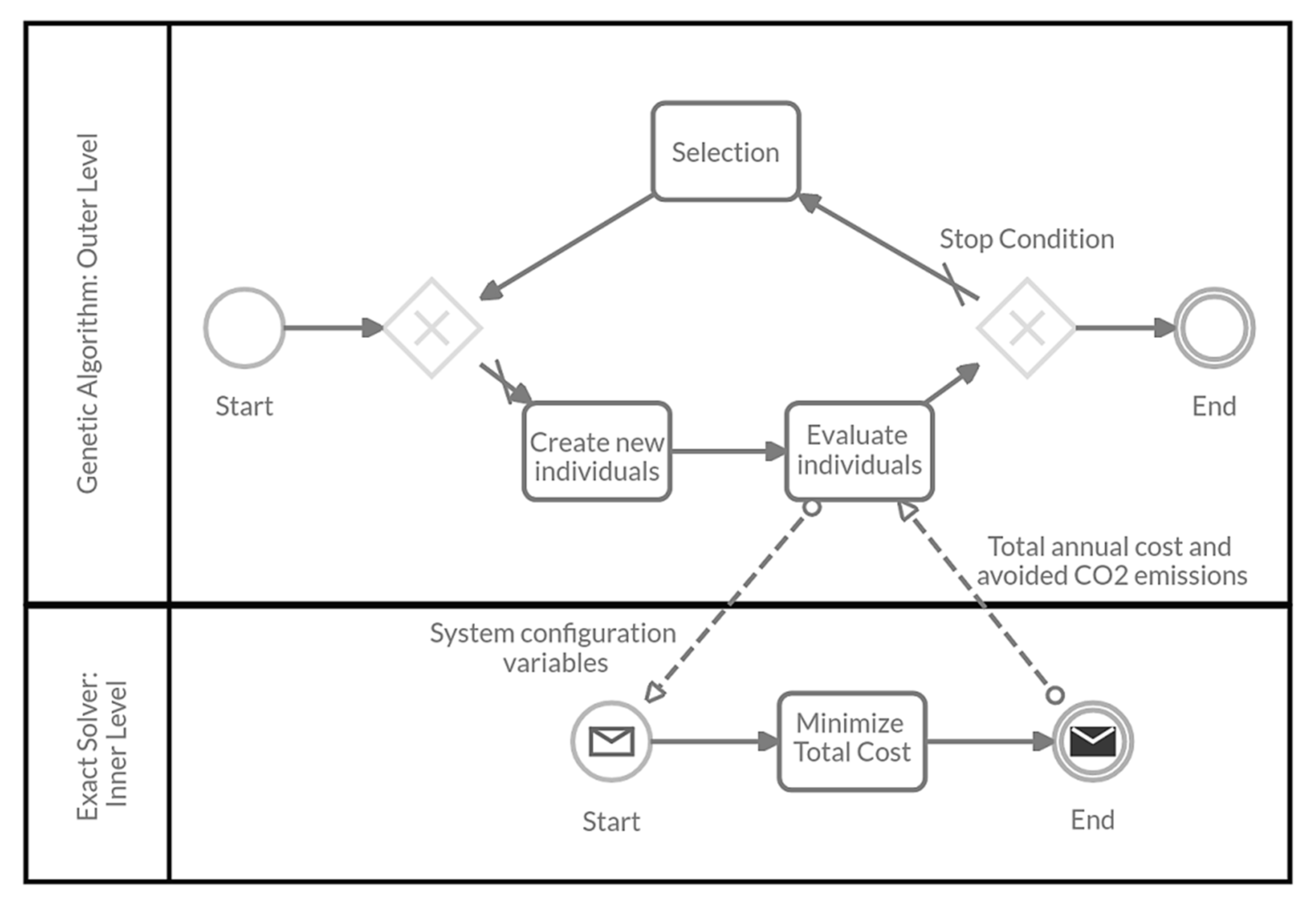
As shown in Figure 5, a simple iteration loop has been defined. During its optimization loop the genetic algorithm assigns the values to the system configuration variables defining the current generation of individuals (i.e., variables X (j, k) and r (k, v) introduced in Section 2). The problem has been set with 40 individuals per generation and 25 generations. The individual evaluation phase is made on the basis of the results of exact solver at the inner level. The latter receives the configuration variables of each individual and, for each of them, it performs the operation optimization using the total annual cost (Cost_TOT, Equation (1)) as objective function.

The optimal solution contains not only the minimum total annual cost allowed by the configuration variables introduced for each individual, but also the equivalent CO₂ emissions and therefore the avoided emissions, with respect to the conventional solution for energy supply. The optimized variable assignment in the inner level is sent back to the outer level to allow the genetic algorithm to determine whether a solution is suitable for guiding the creation of the next generation of solutions, as well as the quantitative indexes of each solution (these indexes are then summarized in the scatter matrix and in the probability density function charts, presented in the following Section 5). The entire loop is repeated until the termination criterion is reached, i.e., when a further evolution of the population does not obtain any appreciable performance improvement, indicated as stop condition in Figure 5. It is worth noting that more than one objective function can be used to evaluate the individual performance, allowing to highlight different convergence stories and to identify the Pareto front. In this case study one second objective function (besides the total annual cost) have been considered: the avoided CO₂ emissions during the year (to be maximized), in order of measuring the environmental impact of the modeled system.

By applying this two-level approach to the case study, i.e., the optimization of the CHP system with district heating for six buildings, the computational times for each solution provided to the inner level were reduced to a mere 3 seconds compared to the previous 26 min required by the direct MILP approach. This means that we could perform 520 design evaluations in the same time without using any parallel computing functionalities of the workstation.

The modeFRONTIER^® software enabled us not only to keep the original MILP model used in the direct approach, but also to integrate it in a hierarchical optimization workflow. After an exploration of different optimization algorithms, we decided to use the non-dominating sorting genetic algorithm NSGA-II, widely discussed in literature [51]. We considered it the most suitable approach for tackling the outer level of this problem in terms of result accuracy and convergence rate. Furthermore, this approach enabled us to use the multi-core processor of the computer and thus perform in parallel multiple inner level runs, which significantly sped up the optimization process. Repeated optimization test runs resulted in the optimal problem solution in less than 15 min with an accurate exploration of the design space.

Given these results, a sub-set of the inner level parameters was transferred to the outer level, i.e., the surfaces of thermal collectors (A_ST (k)) and PV panels (A_PV (k)). In this way the computations at the inner level were further streamlined without this having a negative impact on the outer level, and all design variables have been put in the outer decision level, allowing the genetic algorithm to manage directly the surfaces of thermal collectors and PV panels, in view of both objective functions.

It is worth noting that an easy implementation of the multi-objective approach has been possible because the choice of the objective as the merit function of the genetic algorithm affects only the decision variables of the outer level, not the inner level.

The presence of two objectives in the outer level and only one of those objectives, i.e., cost minimization, at the inner level, may throw the search off balance in favor of this objective. In spite of this apparent drawback, the NSGA-II algorithm is able to maintain the uniformity of the Pareto front. However, we can expect a different quality of exploration between the two tails of the front corresponding to the best values of each of the objectives. The tail of the avoided CO₂ emissions objective will be less explored, but this is not an issue because the most expensive solutions lead to a rather small additional environmental benefit in terms of CO₂ emissions and has thus poor industrial appeal.

5. Results

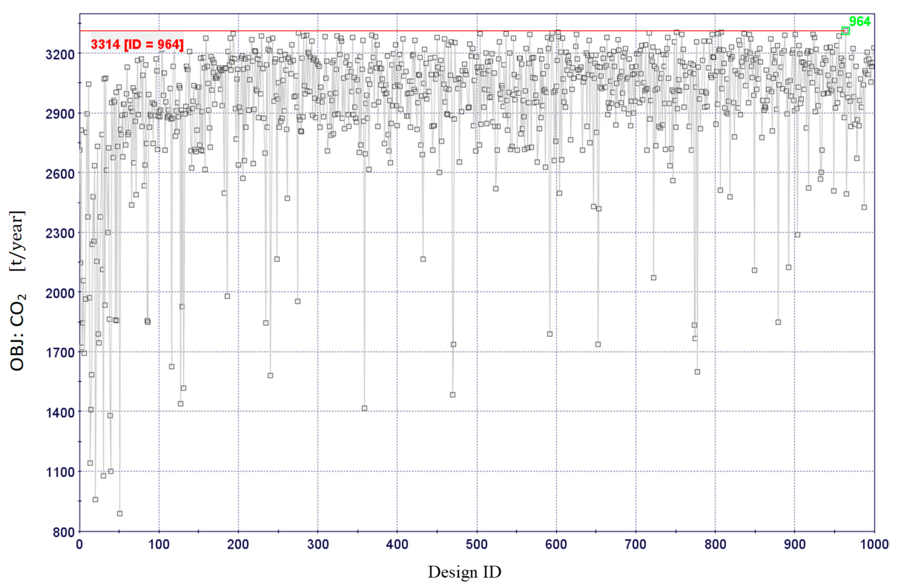
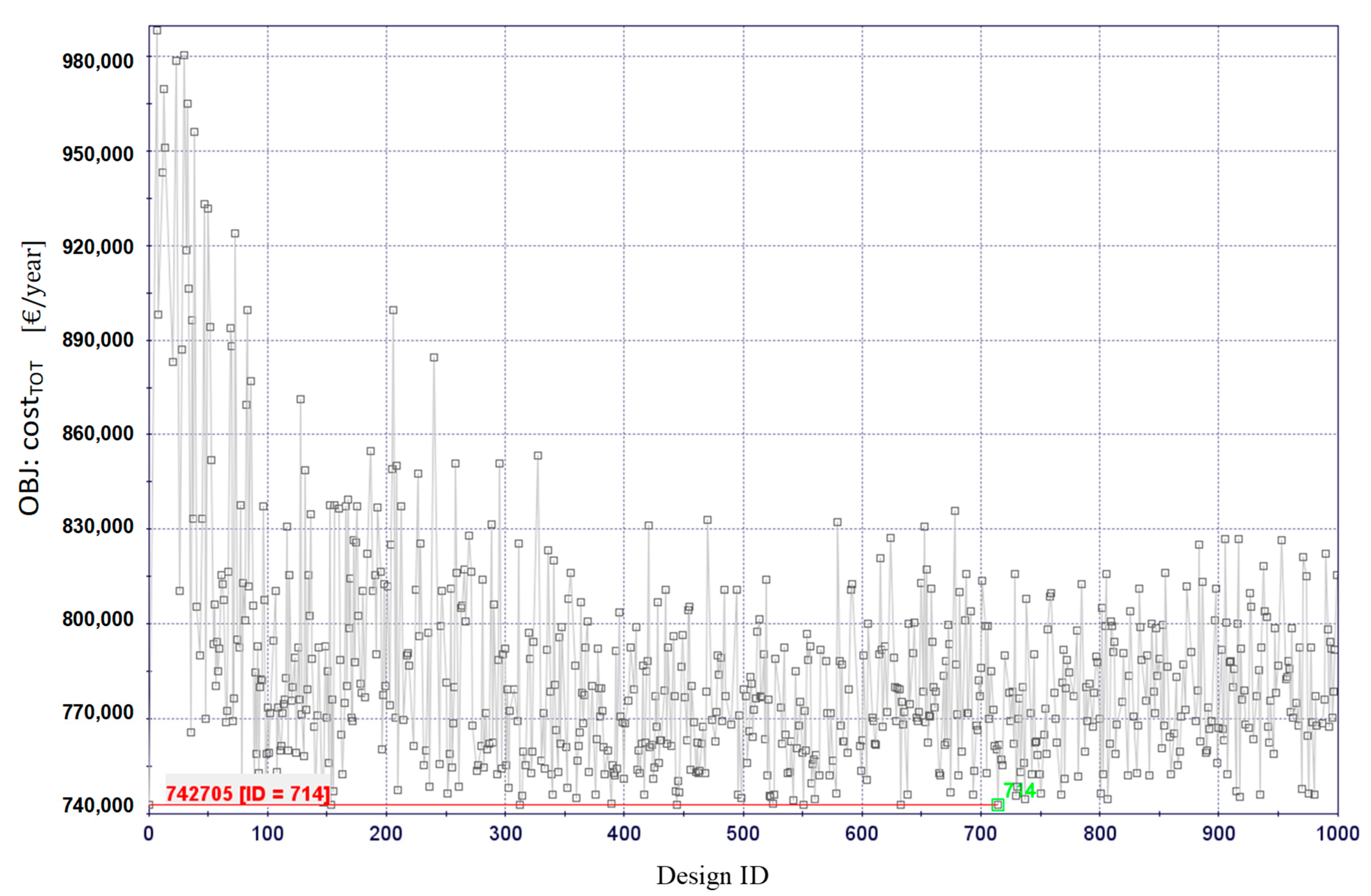
Figure 6 and Figure 7 show the convergence history of the hierarchical optimization of both objectives, i.e., avoided CO₂ emissions and total annual cost. In particular, Figure 6 shows that the maximum CO₂ savings of 3314 t/year has been obtained at iteration number 964 (Design ID), but this solution implies an unacceptable annual cost of 30,383,000 €/year. At this point we performed result post processing to exclude unfeasible solutions from a practical point of view. This consisted in limiting the maximum annual cost to 1,000,000 €/year. With this constraint the new optimal design has been obtained at iteration number 905 (Design ID) with 3241 t/year CO₂ saving.

Figure 7 shows that the minimum annual cost of 742,705 €/year has been obtained at iteration number 714 (Design ID). However, the genetic algorithm had already found a value very similar to this after only about 150 iterations.

The two optimal solutions (ID 714 and 905) are shown in

Table 3. Main results for the optimal total annual cost and for the optimal avoided CO₂ emissions.

Design ID	0 (Reference Conventional) Energy Supply	714	905	419
Total number of TG	0	4	11	9
Location of ICE at building	-	#2	#2	#2
Total number of pipelines in the DHN	0	3	5	4
Total amount of PV panels [m2]	0	600	600	594
Total amount of ST collectors [m2]	0	2	4	10
Total cost [€/year]	796,064	742,705	826,940	788,265
Total cost reduction [€/year]	0	53,359	−30,876	7799
Avoided CO2 emissions [t/year]	0	2714	3241	3186

. The cheapest solution (ID 714) includes 4 micro-gas turbines and the ICE CHP installed near building number 2, three pipeline connections and the maximum allowed area of PV panels. The contribution of the solar thermal collectors in this case is negligible, so that the rational solution is to not install any solar thermal collector. The monetary saving amounts to about 53,000 €/year compared to the reference solution.

One of the main advantages of multi-objective optimization methods is the generation of many feasible trade-off solutions, so the designer can easily identify the best compromise. Approximately 1000 evaluations with NSGA-II have been performed in 8 min and a set of Pareto solutions representing equally valid CHP system configuration alternatives have been identified.

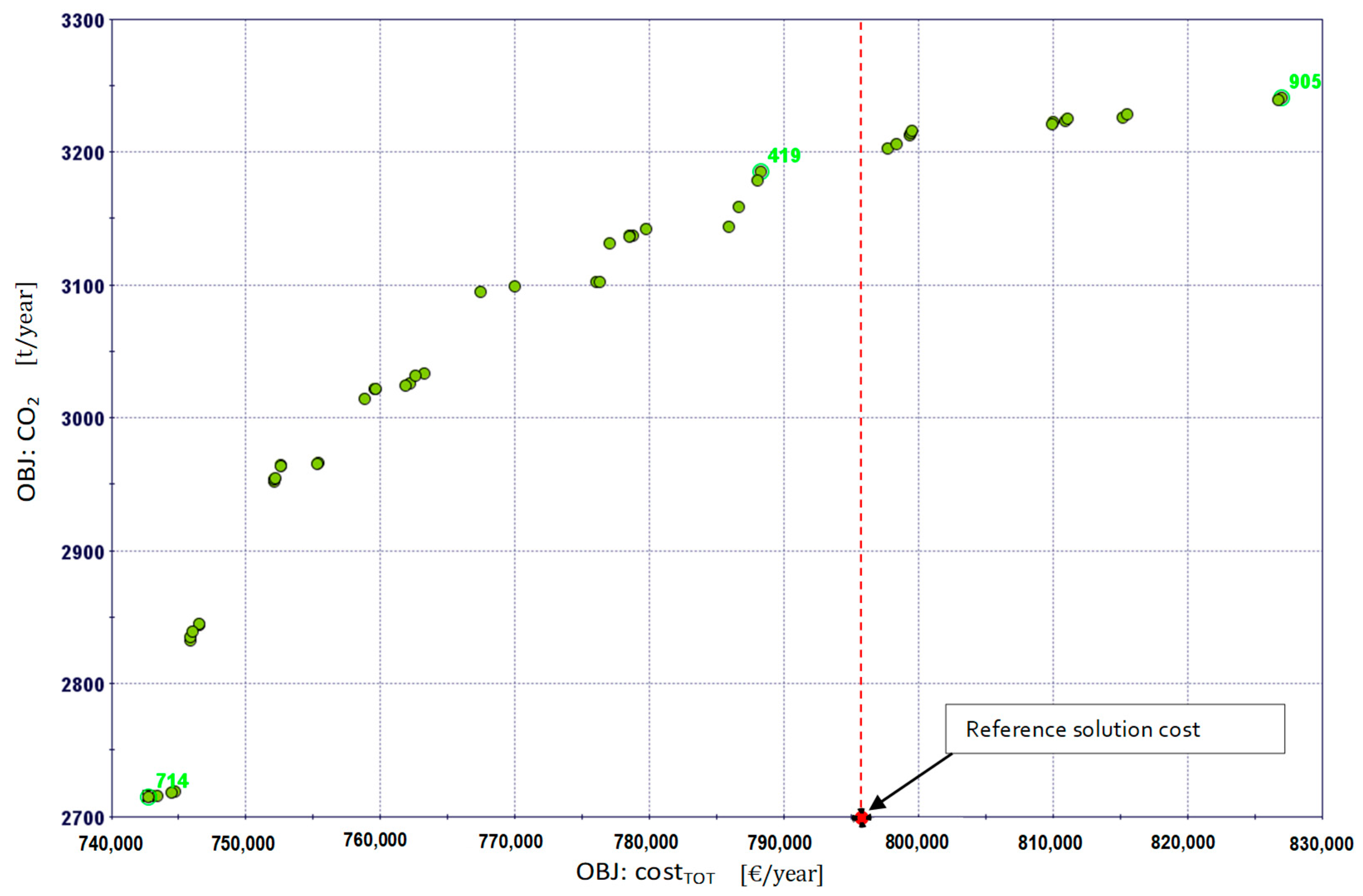
The final Pareto front obtained for the case study is shown on the Scatter Chart in Figure 8. The cost objective (to be minimized) is plotted on the x axis whereas the avoided CO₂ emissions (to be maximized) are plotted on the y axis. The Pareto solutions, displayed as green circles, are well distributed in the design space. The reference solution is represented as a red dot at the bottom of the chart with cost value of 796,064 €/year. However, for the sake of clarity of the comparison it was placed on the x axis even though the CO₂ saving is actually 0 t/year. The solution with ID 905 brings about a CO₂ saving of approximately 3241 t/year with a cost of 826,940 €/year, which is only 30,876 €/year more than the reference solution. For this reason this solution is regarded as the most environmentally friendly (see Table 3). This optimal solution includes the ICE and the maximum number of micro-gas turbine (11) and pipelines (5) among all solutions of the Pareto front. Notice that a different preliminary choice of a bigger ICE, or of allowing two or more ICE to be installed, is expected to reduce the number of mTG in the optimal solution, but this option has been not considered in this study because of the nature of the users which generally requires small and quiet operating cogenerators.

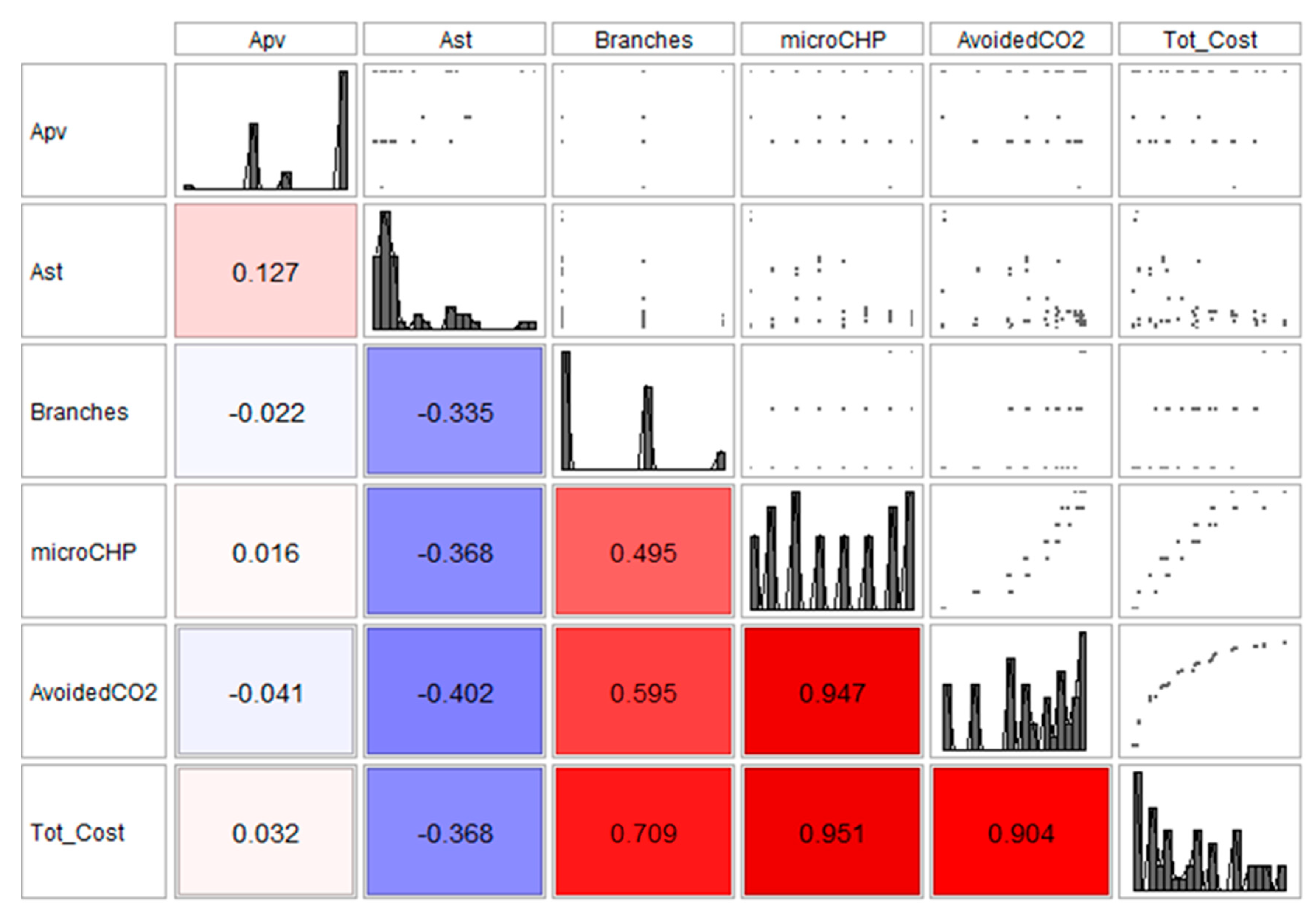
The Scatter Matrix chart available in modeFRONTIER^® (Figure 9) deals in detail with the solutions on the Pareto front and helps us understand the behavior of outer level variables, how they influence each other and how their values are distributed [49]. All input variables of the outer level and the two objectives are plotted on both axes; in the chart, the bottom-left triangular matrix shows the Pearson coefficient for correlations and each colored square shows the strength and the type of correlation (positive or negative) between a variable pair (one plotted on the x axis and the other on the y axis). The up-right triangular matrix shows the same information in graphic form: the higher Pearson coefficients correspond to a more evident correlation in the small picture between two variables in the symmetric position inside the Scatter Matrix. The main diagonal of the Scatter Matrix shows the probability density function for the distribution of variable values in the solutions on the Pareto front, commented in the following.

The two objectives (total annual cost and avoided CO₂ emissions) are strongly positively correlated, as expected, but even more so with the number of micro-CHP units. It is perfectly plausible that the more the CHP components in the plant to be purchased and maintained, the higher the cost, but on the other hand this helps to reduce the CO₂ emissions. These three variables (total cost in particular) are also highly positively correlated with the number of branches (pipelines) of the DHN, but with a lower value of the Pearson coefficient.

A moderate inverse correlation can be observed between the thermal collector surface (A_ST) and all the above mentioned variables. In fact, the more the branches and CHP units in the plant, the less the usefulness of the thermal collectors to satisfy the energy demand of the buildings. On the other hand, the use of solar energy implies a reduction of CHP units and therefore a lower total cost, but also less avoided CO₂ emissions because additional power has to be purchased from the grid.

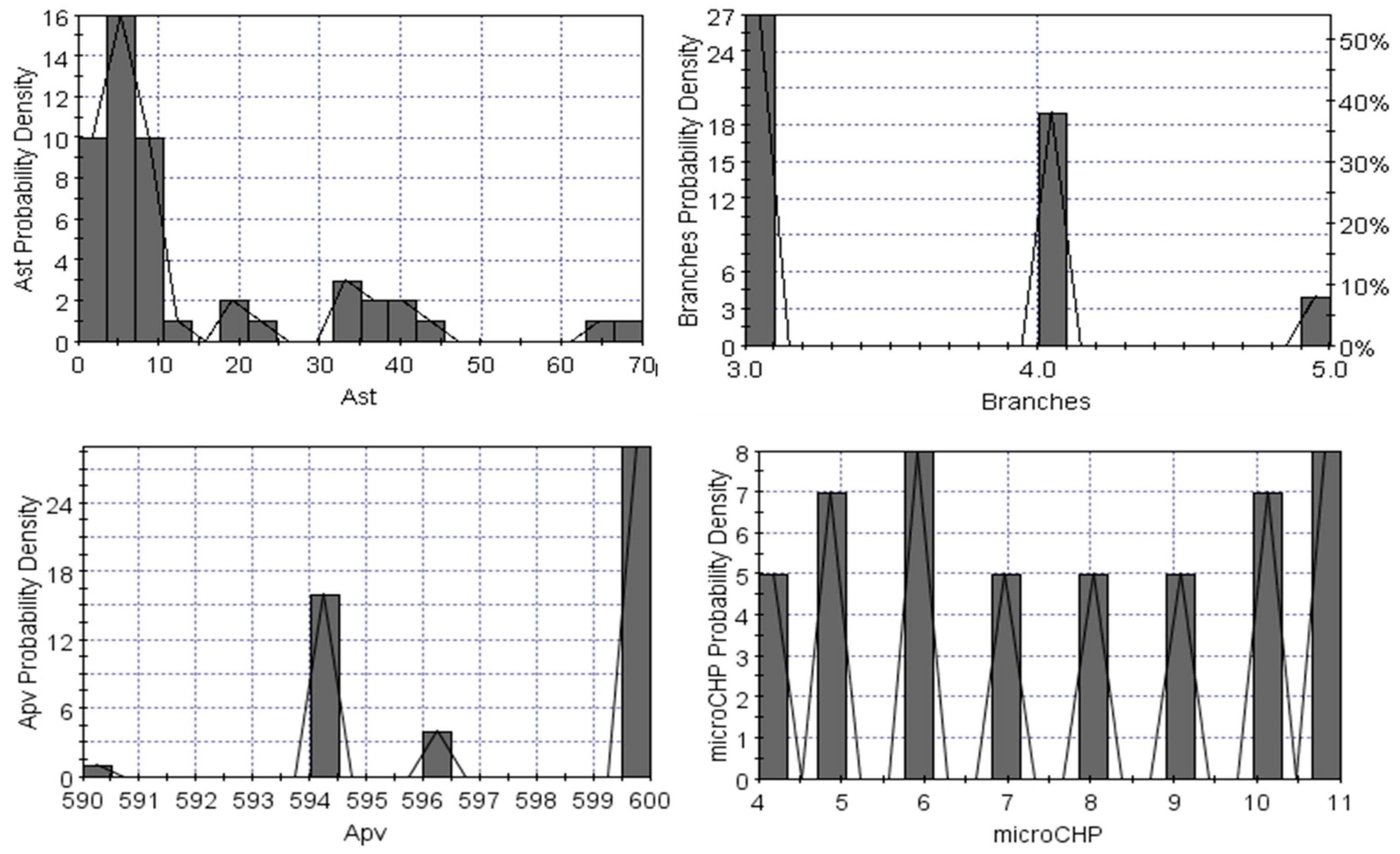
The probability density function charts (Figure 10) reveal that the number of branches is in most cases limited to two mid values, i.e., 3 and 4. In no case has an optimal solution been found for the minimum (i.e., 0) and the maximum (i.e., 8) number of branches.

A significant variability can be observed in the total surface of thermal collectors A_ST (between 0 and 70 m²), although the majority of solutions have the lowest values. Few solar thermal collectors are installed in all optimal solutions because of the high investment costs.

On the contrary, the PV panel range of values is quite restricted: between 590 and 600 m², with more than half optimal configurations having the highest value, because of the strong reduction of costs occurred in recent years for this kind of components.

Finally, we can consider the number of micro-CHP units as the most relevant outer level variable due to their rather uniform distribution on the Pareto front, as shown in Figure 10. From the Pareto front (Figure 8) it can be noted that the solution allowing the maximum CO₂ saving and, at the same time, a reduction of the total cost compared to the reference solution, is ID 419. The main results for this compromise solution are shown in Table 3.

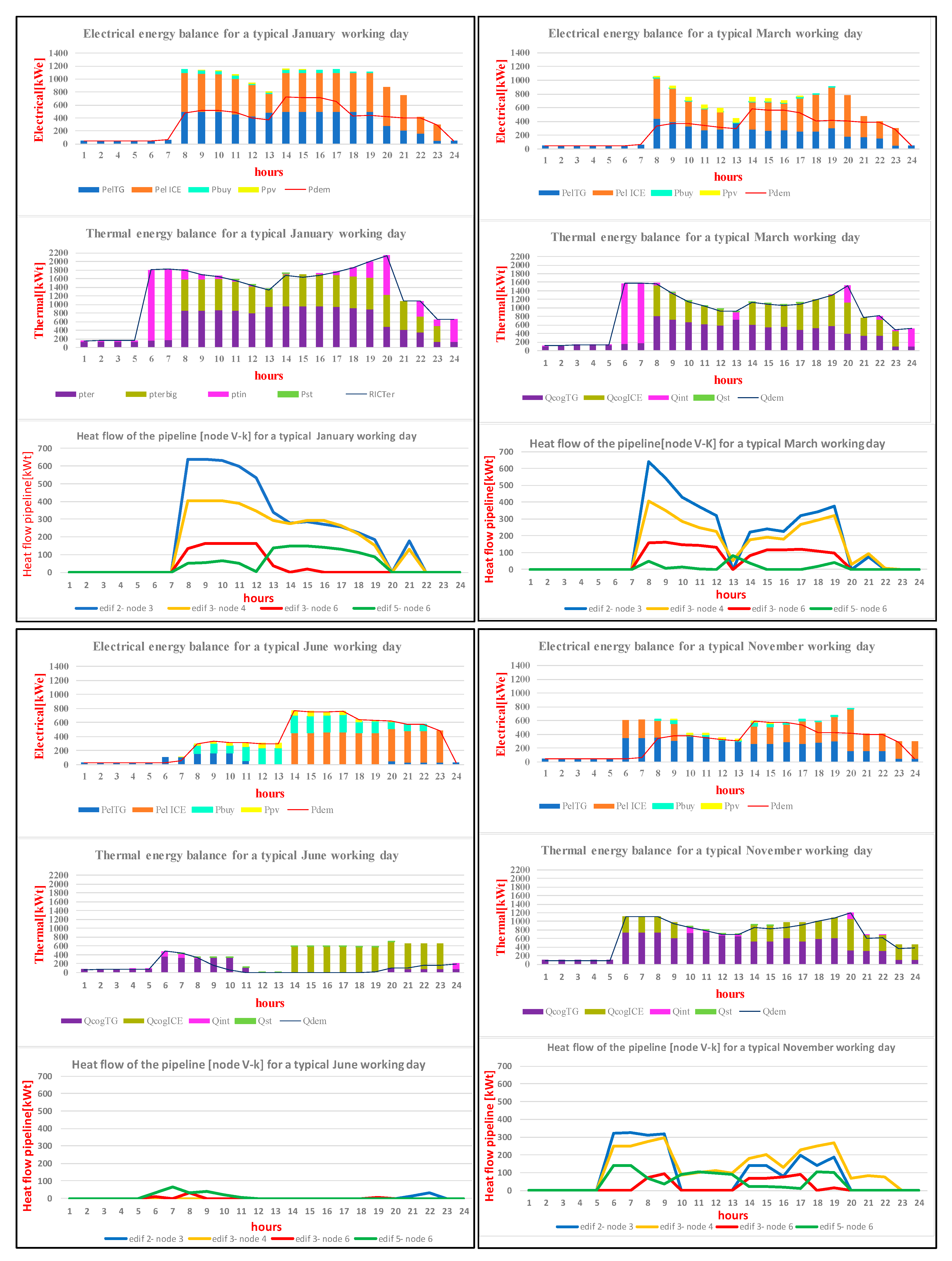
Once one solution has been identified in the Pareto front, the output of the optimization model contains complete information about the optimal structure and operation of the energy system. As an example, Figure 11 shows the electricity, heat and pipelines optimal hourly schedules in 4 typical working days, for the compromise optimal solution ID 419.

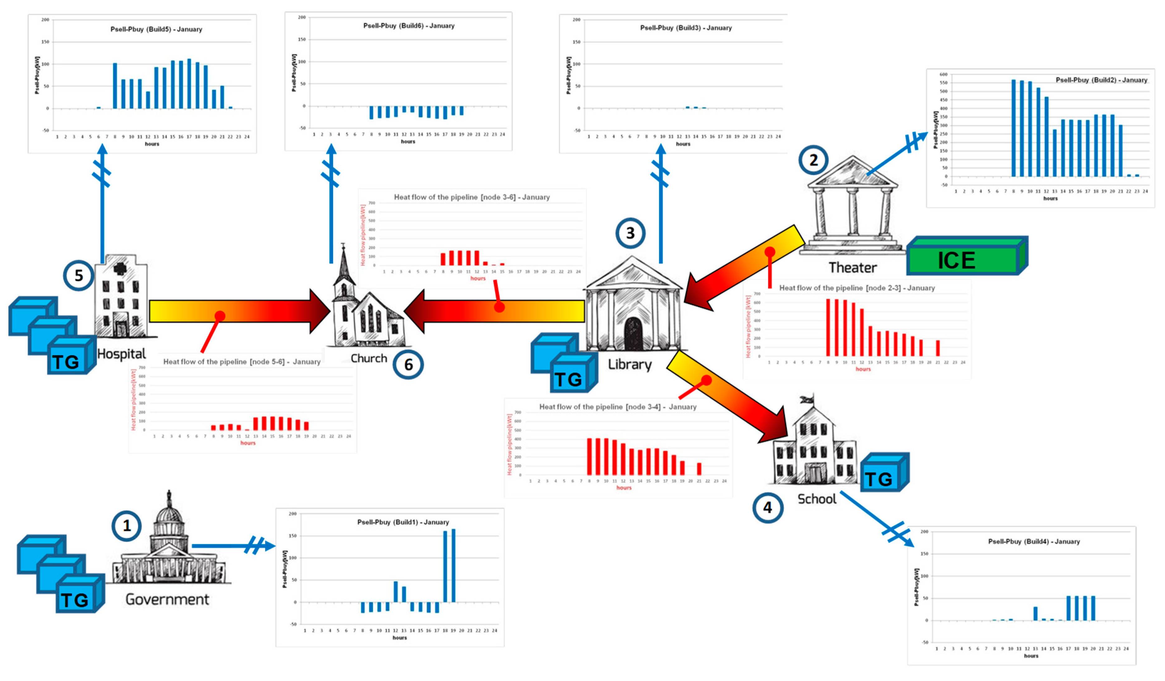
Notice that the electrical and thermal energy values have been aggregated at global system level, even if the solution contains the values of all energy flows exchanged by each building and produced by each cogeneration unit. In Figure 12 the detailed hourly schedules of heat flows through the pipelines and electric energy exchanged with the grid is shown for a typical January working day.

By analyzing the electric energy balance in Figure 11, it can be noted that the whole system produces an excess of energy compared to the electric demand, especially during the winter time; nevertheless, some buildings need, at the same time, to buy electric energy from the grid. Figure 12 shows that this happens in buildings 1 and 6 (during the typical January working day).

Looking at the heat balances, it can be noted that the cogeneration units satisfy almost the whole heat demand; in summer time the ICE is operated at partial load for about 10 h per day and the excess heat is dissipated. The optimal solutions also contain the position of the mGTs and of the pipelines, so that the path of the micro district heating grids can be easily inferred. In particular, for the solution considered, there is only one micro district heating grid and one isolated building (Figure 12). The purpose of the grid is to distribute the heat produced by the ICE in building 2 also to buildings 3, 4 and 6, so that a grid bifurcation is required in site 3. Building 6 is connected to the micro district heating grid, so that it can take advantage of the cogenerated heat even if there are no cogeneration units inside it. The micro district heating grid is operated all the time, except in the summer time. This detailed information can be obtained for each identified solution and for each typical day, providing a basis for knowledge for the design of the complex energy system, taking into account in advance the peculiarities of its optimal management.

The optimal configuration and management are generally both affected by the boundary conditions and the preliminary choices made (mainly by the investment and energy prices, the Carbon Intensity factor, the size and technical characteristics of the components). This clearly means that, adopting different values, the optimization process must be repeated, as shown in previous studies conducted by the authors on similar complex cogeneration systems, leading to optimal configurations also strongly different in terms of number and size of cogenerators and heating network layout; in particular, a sensitivity analysis on the capital recovery factor has been analyzed in [25], another sensitivity analysis on the effect of different supporting policies is presented in [24] and the influence of the Carbon Intensity factor has been studied, by comparing two different cases, in [48]. If the objective is instead to evaluate the total cost and CO₂ emissions values obtained for a certain configuration (for example, the one obtained from a previous optimization) in correspondence with new values of the boundary conditions, the proposed bi-level optimization approach allows to use the internal level only, with a considerable saving in the computational effort.

6. Conclusions

The design and operation optimization of integrated multi-component energy systems generally require a binary variable set to be introduced to describe the existence/absence and the on/off operation status of components and energy connections inside the model. Besides these, other continuous variables have to be introduced for modelling the energy and material flows exchanged among components, as well as other possible design options. In these kinds of optimization problems the decomposition approach, often suggested in literature [15,19,20], may be not best suited, because the discontinuous nature of variables present in many sub-problems can prevent the convergence of the whole problem.

In the case study there are many binary variables in all sub-systems. It is a distributed cogeneration and district heating system, including a set of micro-cogeneration gas turbines (to be located at the energy user sites), a centralized cogeneration system, photovoltaic panels, solar thermal collectors and various district heating pipelines, potentially connecting the users. The existence of each one of these components is related to a binary variable in the optimization problem.

In this paper an innovative approach is presented that allows to exploit the essential positive characteristics of decomposition, overcoming its difficulties by using a bi-level optimization strategy, which involves an outer and an inner level. The outer level configuration was optimized with a genetic algorithm of the commercial optimization software modeFRONTIER^® [50], whereas the inner level was solved with FICO^® Xpress optimization suite [49]. The outer is concerned with all the structural variables of the whole system, including the distribution of the micro CHP units, at the energy user sites, the district heating pipelines of the network and the surface of thermal collectors and PV panels, leaving at the inner level only the MILP problem of the optimal operation of the whole system. In this approach, a multi objective optimization can be easily performed, by introducing a second objective in the outer level only, and the Pareto front can be obtained. The avoided CO₂ emissions have been introduced as a second, environmental objective, besides the minimum annual cost.

Anyhow, the solutions obtained confirm that CHP systems, optimized for the minimum annual cost, can be favorable from both the economic and environmental standpoints. In the case study, the minimum cost solution allows a monetary saving of about 53,000 €/year and a CO₂ saving of about 2700 t/year. A possible environmental-friendly alternative on the Pareto front allows a maximum CO₂ saving of about 3240 t/year, with an additional cost of only 31,000 €/year, compared to the conventional solution.

The presented optimization strategy highlights an important reduction in the computing time compared to the direct implementation of the whole problem in a single level MILP solver; therefore, the expectation is that it could be applied also to more complex systems, in particular to distributed cogeneration systems with far more users and pipelines in the district heating.

From the data analysis, it can be observed that the evolutionary strategy, implemented in the outer optimization level, allows us to obtain a value very close to the actual optimum after a limited number of iterations. The two objectives are strongly positively correlated and they are mostly influenced (even though to different extents) mainly by the number of micro CHPs, and also by the number of pipelines in the district heating network. This fact highlights how the dislocation of the CHP units is the most critical choice, in order to really obtain the economic and environmental advantages which are expected by the cogeneration technology.

In addition, detailed information can be obtained for each identified solution and for each typical day, providing a knowledge basis for the design of the complex energy system, taking into account in advance the peculiarities of its optimal management.

In summary, the proposed method allows the simultaneous optimization of the distributed cogeneration system and the configuration of micro-district heating networks with multiple users, with an innovative approach, applicable to complex systems, allowing a significant reduction of computing time thanks to the proposed two-level optimization procedure.