Demand-Side Management of Smart Distribution Grids Incorporating Renewable Energy Sources

Abstract

The integration of renewable energy resources (RES) (such as wind and photovoltaic (PV)) on large or small scales, in addition to small generation units, and individual producers, has led to a large variation in energy production, adding uncertainty to power systems (PS) due to the inherent stochasticity of natural resources. The implementation of demand-side management (DSM) in distribution grids (DGs), enabled by intelligent electrical devices and advanced communication infrastructures, ensures safer and more economical operation, giving more flexibility to the intelligent smart grid (SG), and consequently reducing pollutant emissions. Consumers play an active and key role in modern SG as small producers, using RES or through participation in demand response (DR) programs. In this work, the proposed DSM model follows a two-stage stochastic approach to deal with uncertainties associated with RES (wind and PV) together with demand response aggregators (DRA). Three types of DR strategies offered to consumers are compared. Nine test cases are modeled, simulated, and compared in order to analyze the effects of the different DR strategies. The purpose of this work is to minimize DG operating costs from the Distribution System Operator (DSO) point-of-view, through the analysis of different levels of DRA presence, DR strategies, and price variations.

1. Introduction

Sustainable development and climate change mitigation are two of the main challenges facing the energy sector. Energy consumption is intrinsically dependent on fossil fuels, since they serve a major portion of energy demand whether through electricity generation, transportation, or other sectors. If mitigation policies pertaining to environmental problems are not emphasized and effectuated, pollutant emissions could increase by approximately 30% over the next years [1,2].

Thus, to achieve the environmental goals stipulated by worldwide governments, increased integration of renewable energy resources (RES) in electricity generation is one of the most efficient solutions. RES are unlimited, endogenous, and have several benefits compared with conventional energy sources (CES), one of which is the reduction of pollutant emissions in the long-term [3].

However, RES are more uncertain and volatile which in great part are due to the unpredictable behavior associated with their primary sources (e.g., wind flow, solar radiation, etc.).

This leads to loss of flexibility in the power system (PS) and eventually reduces reliability and robustness. Moreover, increased RES penetration is accompanied by gradual replacement of conventional combustion vehicles with electric vehicles (EVs). This allows further reduction of pollutant emissions and may also bring benefits to PS by means of increased flexibility and storage capabilities through proper management and interconnection [4,5,6].

In order to minimize negative impacts related to the stochastic behavior of RES, there is a need to evolve from traditional grids to smart grids (SGs) which enable enhanced energy management. In SG there is, among other features, a two-way communication structure giving consumers the possibility of participating actively in proper functioning of the grid [7].

SG energy management can be extended to the microgrid (MG) concept, which is characterized by independent small-scale energy producers, distributed generation (DG), and storage systems. In DG technologies, unlike their centralized counterparts, electricity generation is distributed over different locations. DG allows reducing costs associated with network infrastructures as well as improvement of system flexibility and reliability. In this paradigm, customers can increasingly function as small individual producers, playing an active role in modern electricity grids [8,9].

SG features enable smart devices to control and communicate between various PS elements (e.g., EVs, energy storage, and home energy management systems), enabling the consumers to participate in demand response (DR) programs [10,11].

The main aim of DR is for consumers to adjust their demand according to availability of supply as part of demand-side management (DSM) strategies. Consumers can adjust their electricity consumption either in response to a price change or in return for an incentive. Thus, by introducing DR programs into PS management, system flexibility is improved as well. In this way, consumers become key elements of the network by performing the management from the demand side [12].

In hours of peak demand, DR programs drive customers to reduce their consumption when the electricity market price is substantially high. DR programs can be classified into price-based DR (PBDRs) or incentive-based DR (IBDRs) [13]. PBDRs are voluntary programs in which customers reduce or change their electricity consumption in response to changes in their electricity price. When the difference in price between different periods is significant, customers can shift their loads to periods when the rates are lower or reduce their consumption altogether.

Examples of PBDR include: time-of-use (TOU), real-time pricing (RTP), critical peak pricing (CPP), peak tariff reduction (PTR), variable peak prices (VPP), extreme-day critical peak-price, and extreme-price prices programs [11]. In the case of PTR programs, customers can receive discounts by reducing energy demand during critical peak periods. Moreover, RTP programs are deeply intertwined with the wholesale market price, varying in real-time throughout the day [13].

TOU and RTP are continuously operational, unlike CPP and other programs which are applied during some days of the year under special conditions [14]. For instance, in reference [15], an elasticity-based model was developed on the demand side, where the incentives and penalties of certain DR programs were considered. It was determined that the consumption of each customer varied according to the elasticity of tariffs. The proposed model allowed significant improvement of the load profile and, consequently, customer satisfaction, due to consideration of their benefits.

IBDRs are involuntary programs in which consumers are driven to change their demand by giving an aggregator or operator the power to partially or fully control their load; or signing agreements/commitments to do it themselves when requested, in exchange for some specific incentive payment. IBDR programs include direct load control (DLC), emergency demand response programs (EDRP), capacity market programs (CAP), and interruptible/curtailable (I/C) services. Two others are included in IBDR market clearing programs: demand bidding/buyback (DB), and ancillary services (A/S) market [14].

In CAP, commitments are made in advance that allow the reduction of load and the Independent System Operator (ISO) can use this tool when required. In A/S agreements, customers can make offers to the market. If accepted, they should always be prepared to reduce their load, since the ISO can request the order on short notice. Compliance is rewarded by the payment of incentives [16].

Moreover, demand elasticity is another challenge to overcome in PS with great potential. An example of this is expressed for instance in reference [17], where the concept of demand elasticity as an opportunity in the retail market environment for devising a new bid instrument was investigated. The proposed work was modeled as a Markov decision problem and the implemented search algorithm considered a machine learning technique in order to analyze the price elasticity of demand by predicting the price.

In reference [18], the authors proposed an energy scheduling problem for a household dotted with photovoltaic (PV) systems, considering an online event-triggered energy management algorithm. For scheduling controllable loads, a Lyapunov optimization method was used and a comprehensive analysis was carried out for the minimization of household bill cost.

In reference [19], an approach to connect market-driven DR programs with current demand-driven energy management systems was proposed. A multi-agent system approach was considered and the concept of an energy flexometer was introduced. To this end, a fundamental agent was proposed, considering three different functional blocks based on an Internet-of-Things (IoT) infrastructure.

In previous references the concept of transactive energy was expressed in DR strategies and in the incentives which are necessary to provide to costumers and other PS players. In reference [20], a detailed state-of-the-art review on transactive energy was presented. Moreover, reference [21] also discussed industrial DR practices and transactive energy methodologies. It was expressed that strategies of transaction mechanisms should be supported by both individual behavior and collective interest of the entire system.

Demand response aggregators (DRA) subsequently appear as new entities in electricity markets, acting as intermediaries between consumers and the ISO/distribution system operator (DSO).

With this, ISOs/DSOs play a key role in the peak-load reduction process and contribute to improved PS safety, reducing the negative effects associated with RES uncertainty. From the consumers perspective, DRA are buyers, first assessing their potential demand reduction, and accordingly, offering different contracts (associated with the various aforementioned DR programs), which consumers choose whether or not to accept.

From the ISO/DSO perspective, after assessing DR potential available, DRA submit their bids/proposals [22,23,24,25].

For instance, in reference [22] a DRA model was proposed for the wholesale electricity market. The ISO/DSO initializes DR programs in the day-ahead market and sends the information to DRA who accordingly submit their offers. As such, DRA rely on information provided by both the ISO/DSO and the consumers, in order to maximize DSM services provided.

After reviewing the state-of-the-art literature, this work proposes a DSM model to improve efficiency and reliability with increased integration of RES in electricity distribution systems. The problem is addressed from the DSO point-of-view, unlike most existing approaches in the scientific literature which consider the ISO point-of-view.

In addition, a large portion of existing studies only consider wind power generation, while this work takes into account both wind power and PV. A two-stage stochastic management model was developed with the objective of minimizing the network operational costs from the DSO point-of-view.

DRA are considered, allowing active consumer participation in the day-ahead electricity market, making reduction of costs feasible. For the interpretation and analysis of the results obtained in the modeling of the proposed problem, nine cases studies (with a different number of DRAs, DR programs, and tariffs) are considered for an extensive comparative analysis in order to analyze the effects of different DR strategies.

The manuscript is organized as follows: Section 2 presents the mathematical formulation considered in the proposed model; Section 3 presents the case studies and the results analysis; and Section 4 lists the conclusions and recommendations for future work.

2. Methodology

In this section, the mathematical formulation of the proposed two-stage stochastic model is presented based on a combination of different methods and underlying concepts from references [9,12,26,27,28,29]. RES stochastic parameters are modeled by taking into account several possible scenarios, in order to simulate the different events in real time. DRA are considered, which work as independent entities offering incentives to the consumers and submitting the best consumers’ DR offers to the DSO. Consequently, the DSO chooses the best offers on the day-ahead electricity market. In this process, the main goal of DRA is to provide DR options to consumers, making them aware of their potential flexibility by maximizing their participation in the electricity market. Three strategies are considered for different types consumers change their load demand: LC, LS, and LR. The proposed problem is solved from the DSO point-of-view, whose objective is the minimization of the DG operating costs.

2.1. Objective Function

Minimization of operational costs from the DSO point-of-view is modeled by Equation (1), which is divided into two summation expressions, corresponding to two distinct stages. The first stage incorporates variables related to the day-ahead market, in which decisions made do not change in the next stage. The second stage variables are related to decisions made in the market in real-time which are affected by stochastic variables.

With this, the value of the variables is not always the same, unlike what happens in the first stage, since different scenarios are used to model stochastic behavior. Thus, the probability of occurrence of each scenario varies due to the uncertainty associated with RES (wind and PV). Equation (1) is expressed as follows:

$$\begin{array}{ll}minimize \{F_{cost}=& {\displaystyle {\displaystyle \sum }_{t\in NT}}\left[{\displaystyle {\displaystyle \sum }_{n\in NN}}\left(MC{P}_t·P_{tn}^{PCC}+C_{tn}^{DG}·P_{tn}^{DG}+C_t^{reg}·re{g}_{tn}^{PCC}+CL{R}_{tn}^{LC}+CL{R}_{tn}^{LS}\right)\right]\\ & +{\displaystyle {\displaystyle \sum }_{s\in S}}pro{b}_s\left(C{s}_{ts}^{reg}·reg{s}_{tns}^{PCC}\right)\}\end{array}$$

(1)

2.2. Problem Restrictions

2.2.1. First-Stage Restrictions

In this stage only the restrictions associated with the day-ahead market are considered. The decisions that are taken at this stage do not change in the following one, just as the different RES scenarios are not represented. Equations (2) and (3) represent the active and reactive power balance of the distribution system, respectively. Those are the equilibrium equations for the day-ahead market. $P_{tn}^{PV}$, $Q_{tn}^{PV}$, $P_{tn}^{WF}$ and $Q_{TN}^{WF}$ correspond to the active and reactive PV and wind power, respectively. $L{D}_{tn}^{Act}$ and $L{D}_{tn}^{Rct}$ represent the expected active and reactive load, respectively.

$P_{tnn}^{+}$, $Q_{tnn}^{+}$, $P_{tnn}^{-}$ and $Q_{tnn}^{-}$ correspond to the active and reactive power flow, in the downstream and upstream directions (of the transmission line), respectively. Equation (3) also contains the total reduced load $L{R}_{tn}^{LC}$ and $L{R}_{tn}^{LS}$ considering the LC and LS options, respectively; as well as the total recovered load $L{R}_{tn}^{LR}$.

Equation (4) refers to the voltage balance in the network bus. Equation (5) corresponds to the linearized constraints of active and reactive power, while Equations (6)–(10) represent in a more specific way, the linearization of each of active and reactive power constraint.

Constraints, from Equations (11) and (12), correspond to the technical limits imposed for the entire distribution network, namely the restrictions on the active and reactive power, respectively. Equation (13) represents the power factor constraints for any $\overline{U}$. Equations (14)–(17) correspond to the grid constraints, where limits are set for the power as well as voltage and current in the bus.

$$\begin{array}{ll}{P}_t^{PCC}+{\displaystyle {\displaystyle \sum }_{n\in PV}}{P}_{tn}^{PV}+& {\displaystyle {\displaystyle \sum }_{n\in WF}}{P}_{tn}^{WF}+{\displaystyle {\displaystyle \sum }_{n\in DG}}{P}_{tn}^{DG}+{\displaystyle {\displaystyle \sum }_{n^{\prime }\in NN}}\left(P_{tn{n}^{\prime }}^{+}-P_{tn{n}^{\prime }}^{-}\right)-{\displaystyle {\displaystyle \sum }_{n^{\prime }\in NN}}\left[\left(P_{tn{n}^{\prime }}^{+}-P_{tn{n}^{\prime }}^{-}\right)+R_{n{n}^{\prime }}·I{2}_{tn{n}^{\prime }}\right]\\ & +{\displaystyle {\displaystyle \sum }_{n\in NN}}\left(L{R}_{tn}^{LC}+L{R}_{tn}^{LS}\right)=L{D}_{tn}^{Act}+{\displaystyle {\displaystyle \sum }_{n\in NN}}L{R}_{tn}^{LR}, \forall t,\forall n\end{array}$$

(2)

$$\begin{array}{ll}{Q}_t^{PCC}+{\displaystyle {\displaystyle \sum }_{n\in PV}}{Q}_{tn}^{PV}+& {\displaystyle {\displaystyle \sum }_{n\in WF}}{Q}_{tn}^{WF}+{\displaystyle {\displaystyle \sum }_{n\in DG}}{Q}_{tn}^{DG}+{\displaystyle {\displaystyle \sum }_{n^{\prime }\in NN}}\left(Q_{tn{n}^{\prime }}^{+}-Q_{tn{n}^{\prime }}^{-}\right)-{\displaystyle {\displaystyle \sum }_{n^{\prime }\in NN}}\left[\left(Q_{tn{n}^{\prime }}^{+}-Q_{tn{n}^{\prime }}^{-}\right)+X_{n{n}^{\prime }}·I{2}_{tn{n}^{\prime }}\right]\\ & =L{D}_{tn}^{Rct}, \forall t,\forall n\end{array}$$

(3)

$$V{2}_{tn}-2R_{n{n}^{\prime }}.\left(P_{tn{n}^{\prime }}^{+}-P_{tn{n}^{\prime }}^{-}\right)-2X_{n{n}^{\prime }}·\left(Q_{tn{n}^{\prime }}^{+}-Q_{tn{n}^{\prime }}^{-}\right)-\left(R_{n{n}^{\prime }}^2+X_{n{n}^{\prime }}^2\right)·I{2}_{tn{n}^{\prime }}-V{2}_{t{n}^{\prime }}=0, \forall t,\forall n$$

(4)

$$V{2}_{tn}^{Nom}·I{2}_{tn{n}^{\prime }}={\displaystyle \sum }_{\tau }\left(2\tau -1\right)∆S_{tn{n}^{\prime }}∆P_{tn{n}^{\prime }}+\left(2\tau -1\right)∆S_{tn{n}^{\prime }}∆Q_{tn{n}^{\prime }}, \forall t,\forall n$$

(5)

$$P_{tn{n}^{\prime }}^{+}+P_{tn{n}^{\prime }}^{-}={\displaystyle \sum }_{\tau }∆P_{tn{n}^{\prime }}\left(\tau \right), \forall t,\forall n$$

(6)

$$Q_{tn{n}^{\prime }}^{+}+Q_{tn{n}^{\prime }}^{-}={\displaystyle \sum }_{\tau }∆Q_{tn{n}^{\prime }}\left(\tau \right), \forall t,\forall n$$

(7)

$$∆P_{tn{n}^{\prime }}\left(\tau \right)\le ∆S_{tn{n}^{\prime }}, \forall t,\forall n$$

(8)

$$∆Q_{tn{n}^{\prime }}\left(\tau \right)\le ∆S_{tn{n}^{\prime }}, \forall t,\forall n$$

(9)

$$∆S_{tn{n}^{\prime }}=\frac{V^{Nom}·I_{n{n}^{\prime }}^{Max}}{\tau }, \forall t,\forall n$$

(10)

$$P_{tn{n}^{\prime }}^{+}+P_{tn{n}^{\prime }}^{-}\le V^{Nom}·I_{n{n}^{\prime }}^{Max}, \forall t,\forall n$$

(11)

$$Q_{tn{n}^{\prime }}^{+}+Q_{tn{n}^{\prime }}^{-}\le V^{Nom}·I_{n{n}^{\prime }}^{Max}, \forall t,\forall n$$

(12)

$$P_{tn}^{\overline{U}}.tan\left({cos}^{-1}\left(-\theta \right)\right)\le Q_{tn}^{\overline{U}}\le P_{tn}^{\overline{U}}·tan\left(co{s}^{-1}\left(\theta \right)\right), \forall t,\forall n$$

(13)

$$0\le P_{tn}^{\overline{U}}\le P_{tn}^{\overline{U},Max}, \forall t,\forall n$$

(14)

$${\left(V^{Min}\right)}^2\le V2\le {\left(V^{Max}\right)}^2, \forall t,\forall n$$

(15)

$$V{2}_{tn}^{nom}={\left(V^{Nom}\right)}^2, \forall t,\forall n$$

(16)

$$I{2}_{tm{n}^{\prime }}\le {\left(I_{n{n}^{\prime }}^{Max}\right)}^2, \forall t,\forall n$$

(17)

2.2.2. Demand Response Strategies

As mentioned earlier, DRA can provide three different strategies (LC, LS, and LR) to the consumers, in order to manage their demand and for the DSO to minimize the PS operating costs. In this section, the equations implemented in this model for load reduction and recovery are presented.

For the LC strategy, the consumers reduce their consumption during peak hours, namely between 09:00 and 14:00, and from 18:00 and 22:00. Each LC contract includes different prices $p_{tk}^{LC}$ and different quantity of load $q_{tk}^{LC}$ that consumers can reduce, which vary depending on the contract $k$ and the time $t$ under analysis. These prices act as an incentive that is given to consumers in exchange for modifying their energy demand.

Equation (18) represents the total reduced load using the LC option, where the binary variable $u_{tnk}^{LC}$ takes the value of 1 if the LR is scheduled by the DRA. Equation (19) represents the cost associated with the LC strategy, and this cost is imposed on the DSO. Equations (20) and (21) represent the maximum and minimum duration of the load reduction, where $y_{tnk}^{LC}$ and $z_{tnk}^{LC}$ are binary variables that assume the value of 1 when contract $k$ starts and finishes, respectively.

Equation (22) corresponds to the maximum number of load reductions allowed in one day. Equation (23) represents the start and finish of the provided contract $k$, and Equation (24) ensures that the binary variables are not all equal to 1 simultaneously, preventing a contract to start and finish simultaneously:

$$L{R}_{tn}^{LC}={\displaystyle \sum }_{k\in NK}{q}_{tk}^{LC}·u_{tnk}^{LC}, \forall t,\forall n,\forall k$$

(18)

$$CL{R}_{tn}^{LC}={\displaystyle \sum }_{k\in NK}{q}_{tk}^{LC}·u_{tnk}^{LC}·p_{tk}^{LC}, \forall t,\forall n,\forall k$$

(19)

$${\displaystyle \sum }_{t\in NT}^{t+LR{D}_{nk}^{min, LC}-1}{z}_{tnk}^{LC}\ge y_{tnk}^{LC}, \forall t,\forall n, \forall k$$

(20)

$${\displaystyle \sum }_{t\in NT}^{t+LR{D}_{nk}^{min, LC}-1}{u}_{tnk}^{LC}\ge LR{D}_{nk}^{min, LC}{y}_{tnk}^{LC}, \forall t,\forall n, \forall k$$

(21)

$${\displaystyle \sum }_{t\in NT}{y}_{tnk}^{LC}\le M{N}_{nk}^{LC}, \forall t,\forall n,\forall k$$

(22)

$$y_{tnk}^{LC}-z_{tnk}^{LC}=u_{tnk}^{LC}-u_{nk\left(t-1\right)}^{LC}, \forall t,\forall n,\forall k$$

(23)

$$y_{tnk}^{LC}-z_{tnk}^{LC}\le 1, \forall t,\forall n, \forall k$$

(24)

For the LS strategy, consumers reduce their load in peak hours, however their consumption can be shifted to other times of the day. With this, the load reduced in peak hours can be recovered in the off-peak and valley hours by using the LR strategy.

The LS contract models are similar to LC, since each include several $p_{tk}^{LS}$ prices and quantities of load that can be reduced and shifted to other hours $q_{tk}^{LS}$ according to contract $k$ and time $t$; $T_{tk}^{LS}$ corresponds to a time intervals sets where the load can be shifted to another period, namely from peak periods to off-peak periods.

Equations (25) and (26) correspond to the load that is reduced at peak-hours and that can be shifted to other periods and to the cost associated with that reduction for the DSO, respectively. The binary variable $u_{tnk}^{LS}$ act as an indicator i.e., if there is a load reduction this assumes the value 1. Equation (27) assures to the DRA that the LS contracts are only offered to the consumers in periods where the load can be moved to other hours.

Inequalities (28), (29) represent the maximum and minimum duration of the contracts $k$ and the binary variables $y_{tnk}^{L}S$ and $z_{tnk}^{LS}$ indicate when the contract is started and finished, respectively. Equation (30) corresponds to the maximum number of times that LS contracts may be used in one day. Equations (31) and (32) represent the relations between the binary variables:

$$L{R}_{tn}^{LS}={\displaystyle \sum }_{k\in NK}{q}_{tk}^{LS}·u_{tnk}^{LS}, \forall t,\forall n,\forall k$$

(25)

$$CL{R}_{tn}^{LS}={\displaystyle \sum }_{k\in NK}{q}_{tk}^{LS}·u_{tnk}^{LS}·p_{tk}^{LS}, \forall t,\forall n,\forall k$$

(26)

$$u_{tnk}^{LS}=0, \forall t\notin T_{tk}^{LS}$$

(27)

$${\displaystyle \sum }_{t\in NT}^{t+LR{D}_{nk}^{min, LS}-1}{z}_{tnk}^{LS}\ge y_{tnk}^{LS}, \forall t,\forall n, \forall k$$

(28)

$${\displaystyle \sum }_{t\in NT}^{t+LR{D}_{nk}^{min, LS}-1}{u}_{tnk}^{LS}\ge LR{D}_{nk}^{min, LS}{y}_{tnk}^{LS}, \forall t,\forall n, \forall k$$

(29)

$${\displaystyle \sum }_{t\in NT}{y}_{tnk}^{LS}\le M{N}_{nk}^{LS}, \forall t,\forall n,\forall k$$

(30)

$$y_{tnk}^{LS}-z_{tnk}^{LS}=u_{tnk}^{LS}-u_{nk\left(t-1\right)}^{LS}, \forall t,\forall n,\forall k$$

(31)

$$y_{tnk}^{LS}-z_{tnk}^{LS}\le 1, \forall t,\forall n, \forall k$$

(32)

With regards to the LR strategy, Equation (33) represents the load provided by the LS contracts and is recovered in the off-peak and valley periods, where the binary variable $u_{tnk}^{LR}$ assumes the value 1 if the load is recovered. In addition, $T_{tk}^{LR}$ represents the time intervals set where the load transferred by the LS contracts can be retrieved, and this varies according to contract $k$ and time $t$. In this way, Equation (34) implies that the displaced load of the LS contracts can only be recovered in these periods. Inequality (35) ensures that the LS and LR options do not occur at the same time.

$$L{R}_{tn}^{LR}={\displaystyle \sum }_{k\in NK}{q}_{tk}^{LS}·u_{tnk}^{LR}, \forall t,\forall n,\forall k$$

(33)

$$u_{tnk}^{LR}=0, \forall t\notin T_{tk}^{LR}$$

(34)

$$u_{tnk}^{LR}-u_{tnk}^{LS}\le 1, \forall t,\forall n, \forall k$$

(35)

2.2.3. Second-Stage Restrictions

In the second stage the restrictions are related to the real-time market and the several scenarios used to consider RES uncertainty. Equations (36) and (37) represent the equilibrium for the real-time market corresponding to active and reactive power balance, respectively, and considering the scenarios involved. In the second stage the electricity produced from CES is not considered (only RES). $P{s}_{tns}^{PV}$, $Q{s}_{tns}^{PV}$, $P{s}_{tns}^{WF}$, and $Q{s}_{tns}^{WF}$ represent the active and reactive power of PV and wind farms, respectively. In Equation (36), the market regulation $reg{s}_{tns}^{PCC}$ compensates for RES fluctuations.

Like the first-stage of the problem, in the second-stage the voltage balance in the buses is considered, represented by Equation (38). Equation (39) corresponds to the linearization of active and reactive power. Equations (40)–(43) represent the constraints from the linearization process. Equations (44) and (45) represent the technical limitations of the PS, in particular the limits of active and reactive power, respectively. Equation (46) indicates the limits of the power factor, and Equations (47) and (48) correspond to the grid constraints related with voltage and current in the buses, respectively:

$$\begin{array}{ll}reg{s}_{tns}^{PCC}+& {\displaystyle {\displaystyle \sum }_{n\in PV}}\left(P{s}_{tns}^{PV}-P_{tn}^{PV}\right)+{\displaystyle {\displaystyle \sum }_{n\in WF}}\left(P{s}_{tns}^{WF}-P_{tn}^{WF}\right)+{\displaystyle {\displaystyle \sum }_{n^{\prime }\in NN}}\left(P{s}_{tn{n}^{\prime }s}^{+}-P{s}_{tn{n}^{\prime }s}^{-}\right)-\left(P_{tn{n}^{\prime }}^{+}-P_{tn{n}^{\prime }}^{-}\right)\\ & -{\displaystyle {\displaystyle \sum }_{n^{\prime }\in NN}}\left[\left(P{s}_{tn{n}^{\prime }s}^{+}-P{s}_{tn{n}^{\prime }s}^{-}\right)+R_{n{n}^{\prime }}·I2s_{tn{n}^{\prime }s}\right]-\left[\left(P_{tn{n}^{\prime }}^{+}-P_{tn{n}^{\prime }}^{-}\right)+R_{n{n}^{\prime }}·I{2}_{tn{n}^{\prime }}\right]=0, \forall t,\forall n, \forall s\end{array}$$

(36)

$$\begin{array}{ll}Q{s}_{tns}^{PCC}+& {\displaystyle {\displaystyle \sum }_{n\in PV}}\left(Q{s}_{tns}^{PV}-Q_{tn}^{PV}\right)+{\displaystyle {\displaystyle \sum }_{n\in WF}}\left(Q{s}_{tns}^{WF}-Q_{tn}^{WF}\right)+{\displaystyle {\displaystyle \sum }_{n^{\prime }\in NN}}\left(Q{s}_{tn{n}^{\prime }s}^{+}-Q{s}_{tn{n}^{\prime }s}^{-}\right)-\left(Q_{tn{n}^{\prime }}^{+}-Q_{tn{n}^{\prime }}^{-}\right)\\ & -{\displaystyle {\displaystyle \sum }_{n^{\prime }\in NN}}\left[\left(Q{s}_{tn{n}^{\prime }s}^{+}-Q{s}_{tn{n}^{\prime }s}^{-}\right)+X_{n{n}^{\prime }}·I2s_{tn{n}^{\prime }s}\right]-\left[\left(Q_{tn{n}^{\prime }}^{+}-Q_{tn{n}^{\prime }}^{-}\right)+X_{n{n}^{\prime }}·I{2}_{tn{n}^{\prime }}\right]=0, \forall t,\forall n, \forall s\end{array}$$

(37)

$$\begin{array}{ll}V2s_{tns}& -2R_{n{n}^{\prime }}·\left(P{s}_{tn{n}^{\prime }s}^{+}-P{s}_{tn{n}^{\prime }s}^{-}\right)-2X_{n{n}^{\prime }}·\left(Q{s}_{tn{n}^{\prime }s}^{+}-Q{s}_{tn{n}^{\prime }s}^{-}\right)\\ & -\left(R_{n{n}^{\prime }}^2+X_{n{n}^{\prime }}^2\right)·I2s_{tn{n}^{\prime }s}-V2s_{t{n}^{\prime }s}=0, \forall t,\forall n, \forall s\end{array}$$

(38)

$$V{2}_{tn}^{Nom}·I2s_{tn{n}^{\prime }s}={\displaystyle \sum }_{\tau }\left(2\tau -1\right)∆S_{tn{n}^{\prime }}∆P{s}_{tn{n}^{\prime }s}+\left(2\tau -1\right)∆S_{tn{n}^{\prime }}∆Q{s}_{tn{n}^{\prime }s}, \forall t,\forall n, \forall s$$

(39)

$$P{s}_{tn{n}^{\prime }s}^{+}+P{s}_{tn{n}^{\prime }s}^{-}={\displaystyle \sum }_{\tau }∆P{s}_{tn{n}^{\prime }s}\left(\tau \right), \forall t,\forall n, \forall s$$

(40)

$$Q{s}_{tn{n}^{\prime }s}^{+}+Q{s}_{tn{n}^{\prime }s}^{-}={\displaystyle \sum }_{\tau }∆Q{s}_{tn{n}^{\prime }s}\left(\tau \right), \forall t,\forall n, \forall s$$

(41)

$$∆P{s}_{tn{n}^{\prime }s}\left(\tau \right)\le ∆S_{tn{n}^{\prime }}, \forall t,\forall n, \forall s$$

(42)

$$∆Q{s}_{tn{n}^{\prime }s}\left(\tau \right)\le ∆S_{tn{n}^{\prime }}, \forall t,\forall n, \forall s$$

(43)

$$P{s}_{tn{n}^{\prime }s}^{+}+P{s}_{tn{n}^{\prime }s}^{-}\le V^{Nom}·I_{n{n}^{\prime }}^{Max}, \forall t,\forall n, \forall s$$

(44)

$$Q{s}_{tn{n}^{\prime }s}^{+}+Q{s}_{tn{n}^{\prime }s}^{-}\le V^{Nom}·I_{n{n}^{\prime }}^{Max}, \forall t,\forall n, \forall s$$

(45)

$$P{s}_{tns}^{\overline{U}}·tan\left({cos}^{-1}\left(-\theta \right)\right)\le Q{s}_{tns}^{\overline{U}}\le P{s}_{tns}^{\overline{U}}·tan\left(co{s}^{-1}\left(\theta \right)\right), \forall t,\forall n, \forall s$$

(46)

$${\left(V^{Min}\right)}^2\le V2s\le {\left(V^{Max}\right)}^2, \forall t,\forall n, \forall s$$

(47)

$$I2s_{tm{n}^{\prime }s}\le {\left(I_{n{n}^{\prime }}^{Max}\right)}^2, \forall t,\forall n, \forall s$$

(48)

3. Case Studies and Results Analysis

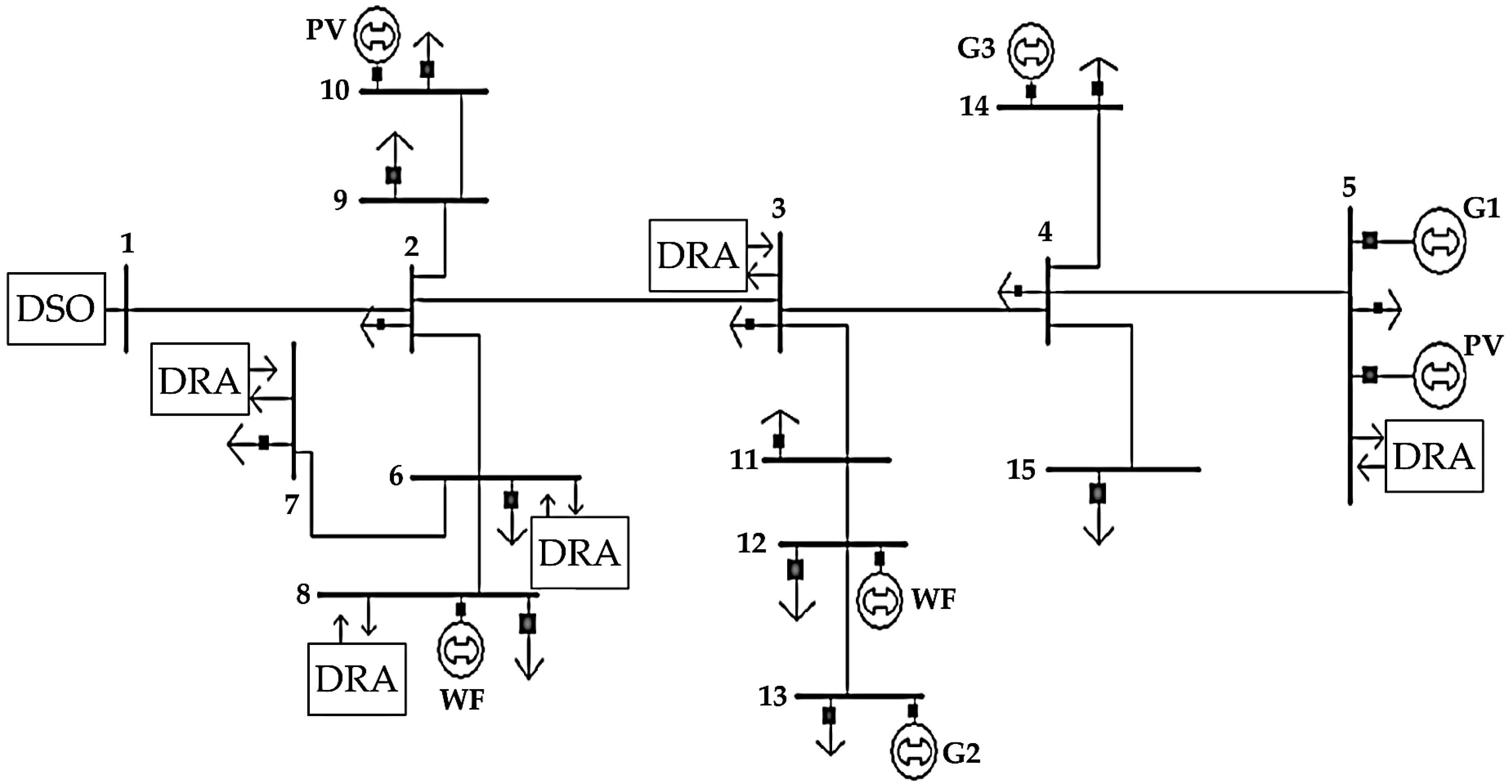
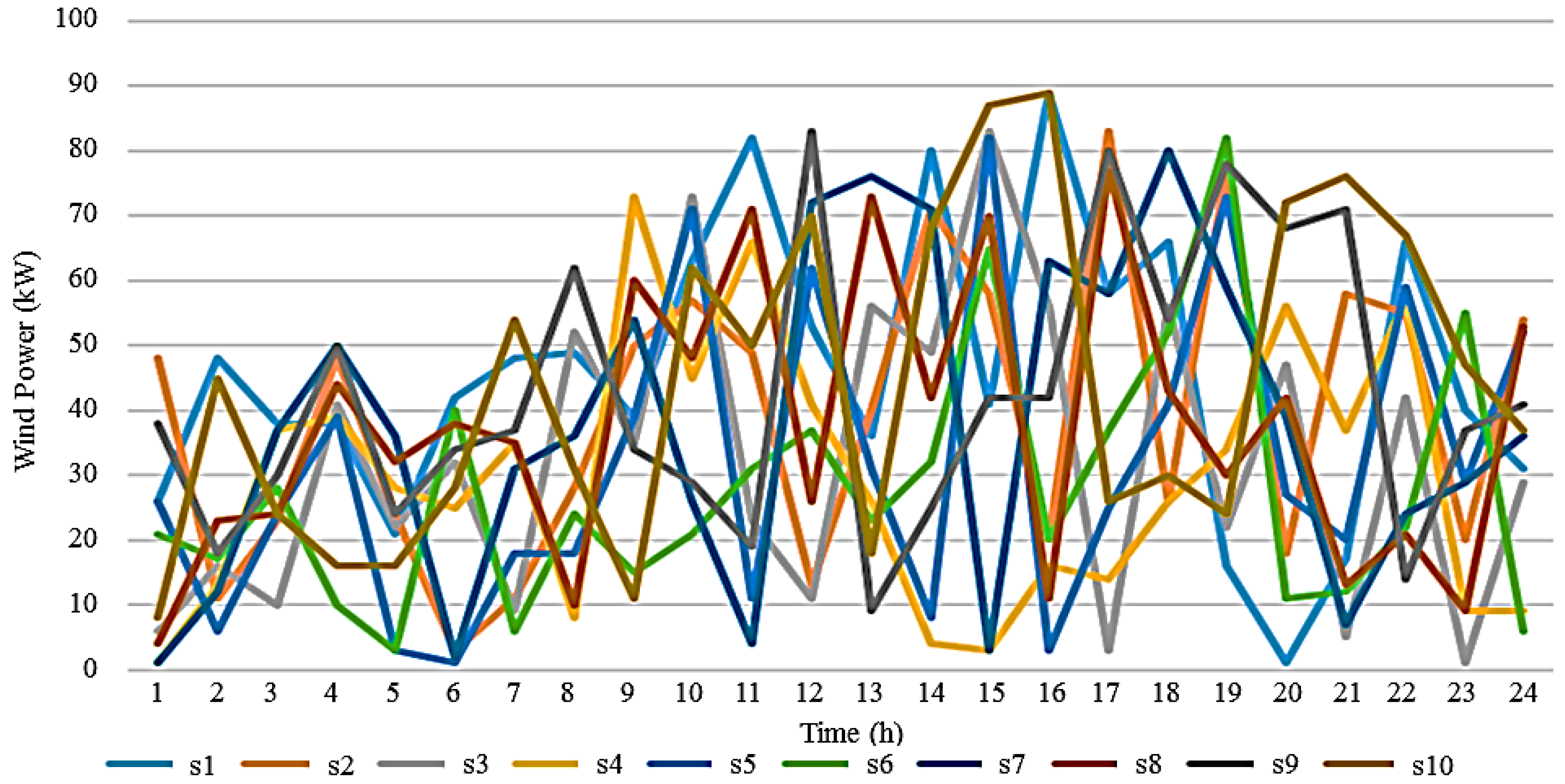
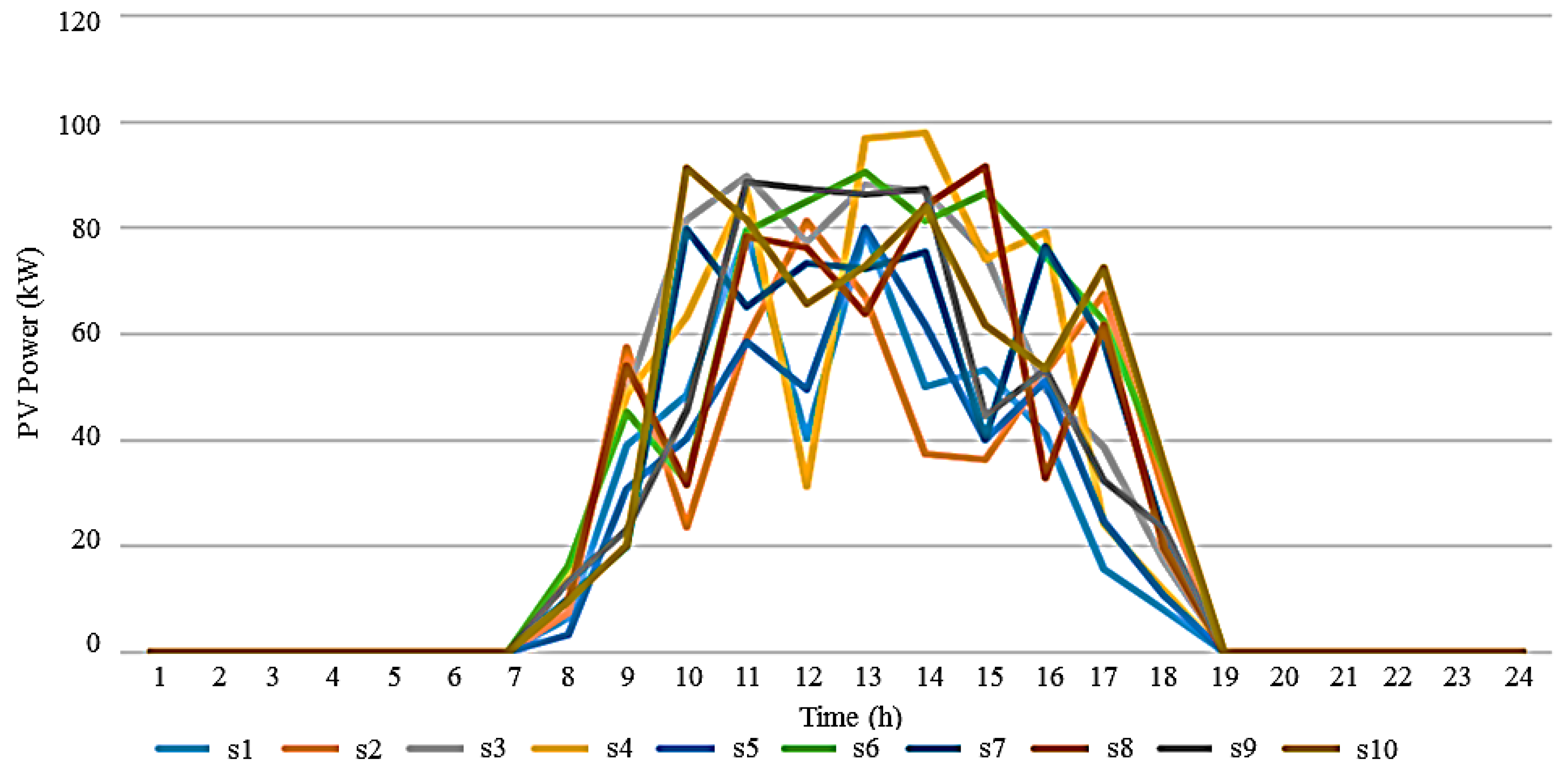
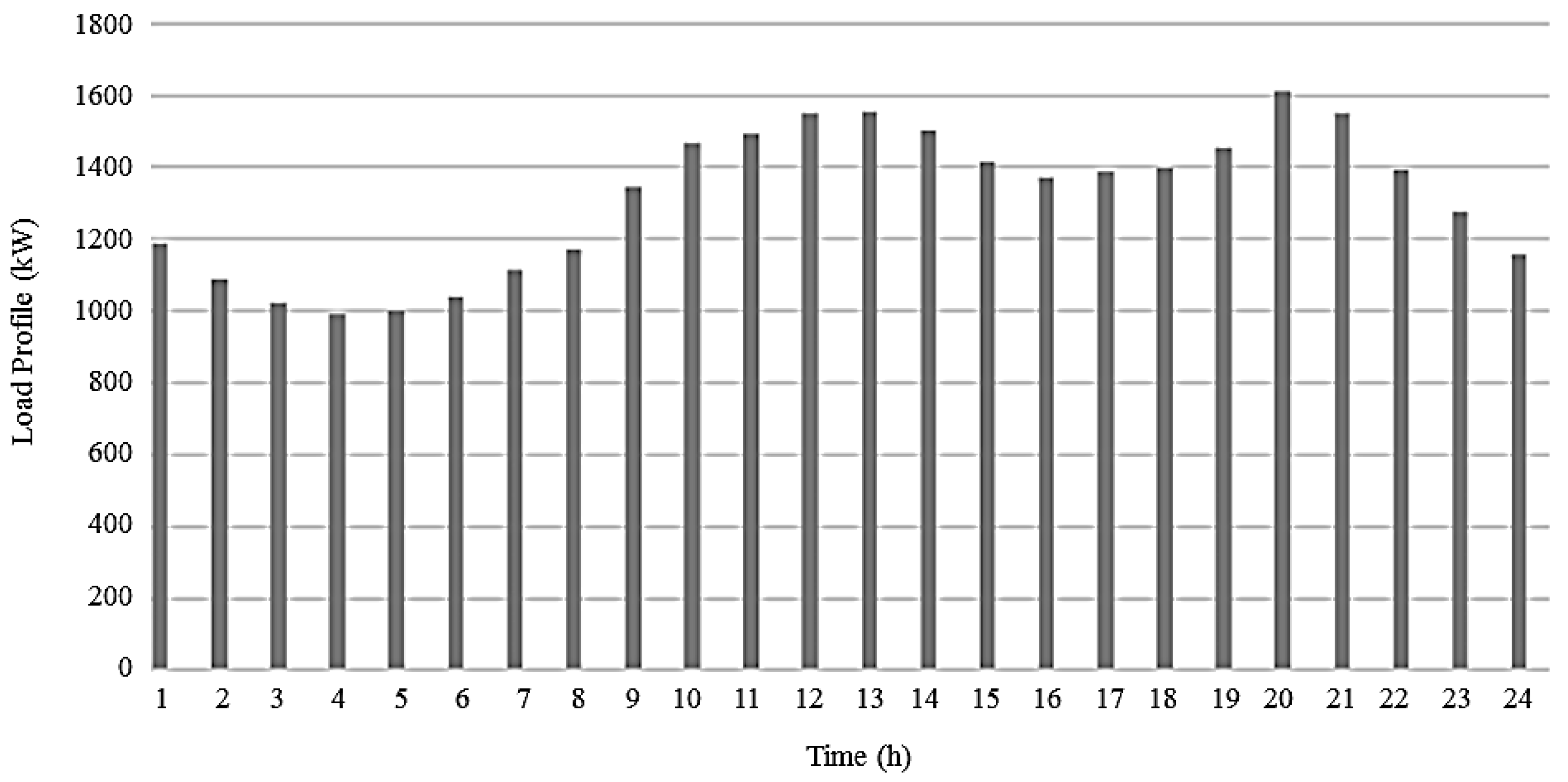
3.1. Details, Data, and System Considered

The model proposed in the previous section was implemented using the General Algebraic Modeling System (GAMS) which uses the mixed-integer linear programming (MILP) package CPLEX (Version 12, IBM ILOG, Sunnyvale, CA, USA). [30] The implementation was performed on a common PC (8 GB RAM, Intel Core i5 2.7 GHz, Windows 7 OS). Compilation time required was less than 3 s. Pre- and post-processing of the results was performed in MS Excel.

The proposed model was tested on the 15-bus distribution grid shown in Figure 1. The distribution grid includes three CES units (micro-turbines), two wind farms and two PV systems. The upstream grid (DSO/ISO operation) is connected to bus 1, from which purchase of electricity is possible in the case of failure in local production (e.g., CES unit failure or RES sudden fluctuation). CES units (listed in

Table 1. Characteristics of conventional generation units.

CES Unit (Bus #)	Power (kW)
	${\mathit{P}}^{\mathit{M}\mathit{i}\mathit{n}}$	${\mathit{P}}^{\mathit{M}\mathit{a}\mathit{x}}$
1 (Bus 05)	23.00	230.00
2 (Bus 13)	69.00	690.00
3 (Bus 14)	46.00	460.00

) are connected to buses 5, 13, and 14. Wind farms are connected to buses 8 and 12.

The Weibull distribution was used assumed for wind speed and afterwards a computational model of the stochastic variables is used to obtain expected wind speeds for each hour and assigning then to a Rayleigh distribution function. Thus, a probability distribution function (PDF) for each of the scenarios is obtained. Finally, the number of scenarios was reduced to 10 (corresponding to the second-stage stochastic problem), which are shown in Figure 2.

Each scenario has a different probability as expressed in

Table 2. Probability of each wind power scenario considered.

Scenario	1	2	3	4	5	6	7	8	9	10
Probability (%)	10.90	9.60	12.40	14.40	2.80	6.40	5.20	17.70	17.80	2.80

, from which the corresponding expected hourly values of wind power generation (used in the first-stage problem) can be calculated and are shown in Figure 3. Those are the values used by the DSO for decision-making and day-ahead electricity market offerings. It should be noted that the historical data used in the PV and wind power production modeling were extracted from [31].

PV systems are connected to buses 5 and 10. As with wind farms, PV are also associated with uncertainties due to the variation of solar energy (e.g., radiation variation, clouds, etc.). For PV power modeling, a Beta distribution was used for solar irradiance. The resulting data was saved in the computation module of the stochastic variables, where various scenarios are created taking into account the historical data collected.

Ten different PV power scenarios were considered with their respective probabilities, in order to model the stochasticity, which are represented in Figure 4 and

Table 3. Probability of each PV power scenario considered.

Scenario	1	2	3	4	5	6	7	8	9	10
Probability (%)	13.30	6.70	4.60	8.10	16.30	14.20	9.40	14.20	4.20	9.00

, respectively. Like wind power, the scenarios were considered in the second-stage of the stochastic model and the expected PV power production was used in the first-stage of the problem, which is shown in Figure 5.

For incorporation of DRA, two distinct cases were modeled. The first case considered three DRA located in the buses 3, 7 and 8. The second case was considered 5 DRA, located in the buses 3, 5, 6, 7, and 8. In this sense, the PS network shown previously in Figure 1 corresponds to the second case. The load curve is divided into different periods: valley period, off-peak period, and peak-period. The valley period corresponds to the time interval between 01:00 and 08:00, and 23:00 and 24:00.

The off-peak period corresponds to the time interval between 15:00 and 17:00. Finally, the peak-periods refer to the intervals between 09:00 and 14:00, and 18:00 and 22:00. The peak load corresponds to 1609 kW. The load curve considered in this study is shown Figure 6.

The electricity prices are shown in Figure 7. As expected, the electricity prices are higher during peak-hours (i.e., when the demand is higher), while in the valley periods the electricity prices are lower. The most expensive electricity tariff is 0.53 €/kWh and corresponds to the interval between 19:00 and 22:00. The cheapest tariff is 0.26 €/kWh between 3:00 and 5:00. In off-peak periods, namely between 15:00 and 17:00, the electricity price is about of 0.42 €/kWh.

3.2. Case Studies

In order to verify the influence of the DRA in the proposed model, different case studies are considered with DRA distributed in three and five buses. Different DR strategies are tested, where contract prices have a 30% of variation between each other. Case 1, which corresponds to the modeling of the problem without the presence of DRA (i.e., without DR strategies) is considered as a base-case for the comparison with the remaining ones. The load curve is shown in Figure 6.

Cases 2 and 3 consider the use of DRA in three and five buses, respectively, with LC contracts offered to the consumers. For cases 4, 5 and 6, DRA are used in three buses, with LS contracts offered to consumers without price changes (case 4), with a 30% increase (case 5) and a 30% reduction (case 6). The cases 7, 8, and 9 follow the same order as 4, 5, and 6 but with DRA used in five buses instead of three.

The different cases are detailed in

Table 4. Summary of case studies analyzed.

Case	Case Description	DR Contract Type	Tariffs	DRA Buses
1	No DR (Base Case)	-	-	-
2	DRA in 3 buses with LC contracts.	LC	+0%	3
3	DRA in 5 buses with LC contracts.	LC	+0%	5
4	DRA in 3 buses with LS contracts and normal electricity tariffs.	LS	+0%	3
5	DRA in 3 buses with LS contracts and 30% electricity tariffs higher.	LS	+30%	3
6	DRA in 3 buses with LS contracts and 30% electricity tariffs lower.	LS	−30%	3
7	DRA in 5 buses with LS contracts and normal electricity tariffs.	LS	+0%	5
8	DRA in 5 buses with LS contracts and 30% electricity tariffs higher.	LS	+30%	5
9	DRA in 5 buses with LS contracts and 30% electricity tariffs lower.	LS	−30%	5

and the respective costs for the various cases studies are shown in

Table 5. Operation and DR Costs for each case study.

Case	Total Operation Cost (€)	DR Cost (€)
1	1014.30	0
2	1053.40	67.80
3	1307.30	107.90
4	1046.50	90.20
5	1064.90	71.90
6	1016.60	69.90
7	1023.50	146.80
8	1055.70	105.70
9	977.50	117.70

. In this manner, the cases where there is no modification of prices are used to compare with the cases where there is an increase or decrease of 30%. This is done in order to verify the influence of price variation on the load profile.

Thus, through the analysis of the different cases and the various comparisons made between them, it is possible to observe how the DSO responds to the use of DRA in three or five buses, as well as to the price variation of the contracts provided by the DRA. The information about the LC contract is shown in

Table 6. LC contract information to DRA distributed in 3 and 5 buses.

Contract	LC Period (h)	Quantity (kW)	Price (€/kW)
K1	09:00–14:00 18:00–22:00	16.10 18.40	0.02 0.03
K2	09:00–14:00 18:00–22:00	18.40 21.85	0.03 0.04
K3	09:00–14:00 18:00–22:00	21.85 23.00	0.04 0.05

and

Table 7. Additional LC contract information.

Contract	Maximum LC per Day	Maximum Time of Load Reduction (h)	Minimum Time of Load Reduction (h)
K1	1	9	4
K2	1	9	4
K3	1	9	4

.

In Table 6, the quantity of load and the respective price for each period are described for each contract. Meanwhile, Table 7 shows the maximum and minimum time duration reduction of the load as well as the maximum number of contracts assigned per day for each consumer. Moreover, the data of the LS contracts are shown in

Table 8. LS contract information to DRA distributed in 3 and 5 buses.

Contract	K1	K2	K3
LS period (h)	09:00–14:00 18:00–22:00	09:00–14:00 18:00–22:00	09:00–14:00 18:00–22:00
LR period (h)	02:00–07:00	15:00–17:00 23:00–00:00	02:00–07:00 15:00–17:00
Quantity (kW)	16.10	18.40	20.70
Normal Price (€/kW)	0.020	0.030	0.040
Price 30% higher (€/kW)	0.026	0.039	0.052
Price 30% lower (€/kW)	0.014	0.021	0.028
Maximum LS per day	1	1	1
Maximum time of load reduction (h)	9	9	9
Minimum time of load reduction (h)	4	4	4

, where the LS and LR periods are presented as well as the quantity of load and the prices considered in the different cases.

3.3. Results Analysis

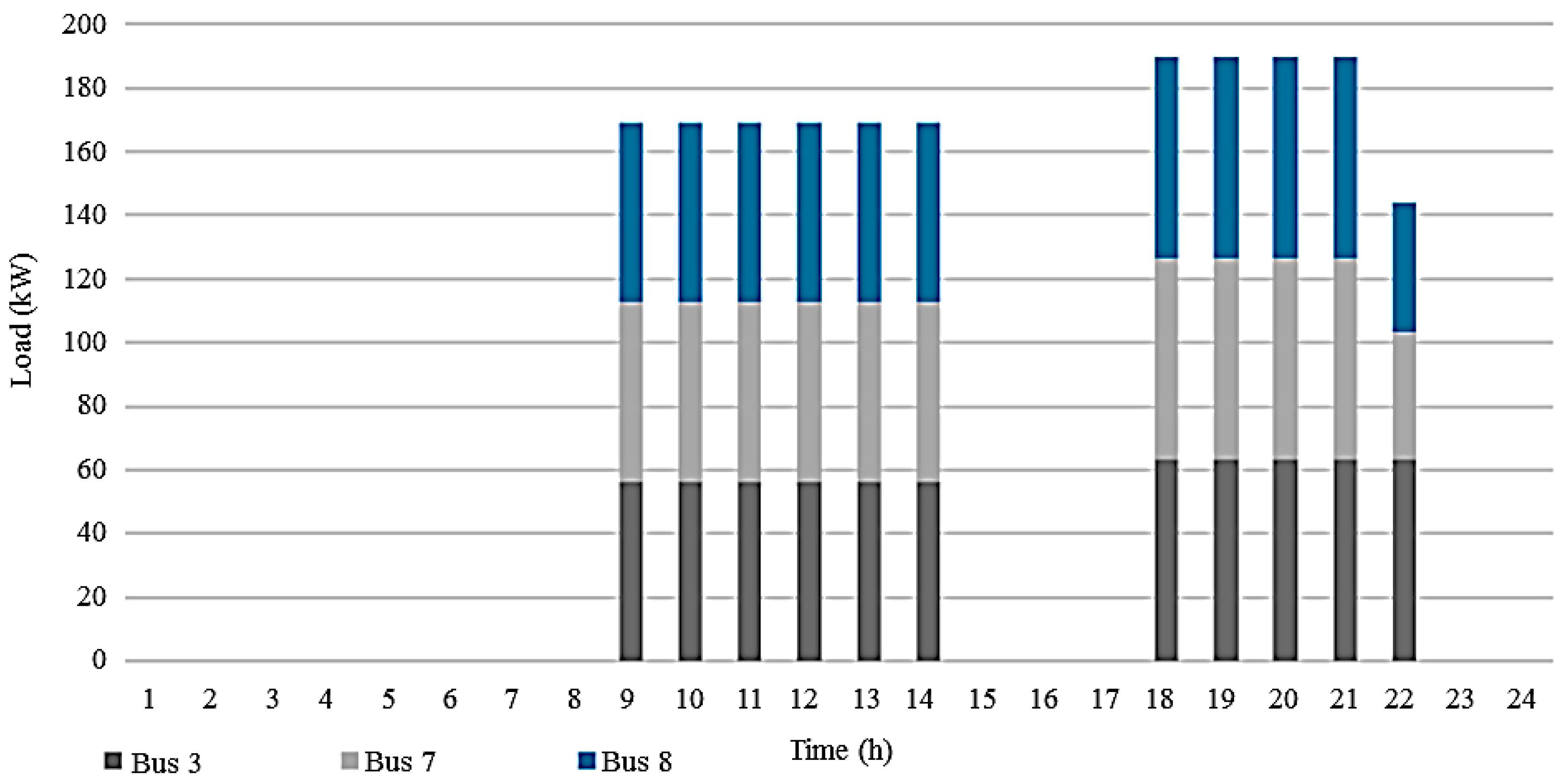
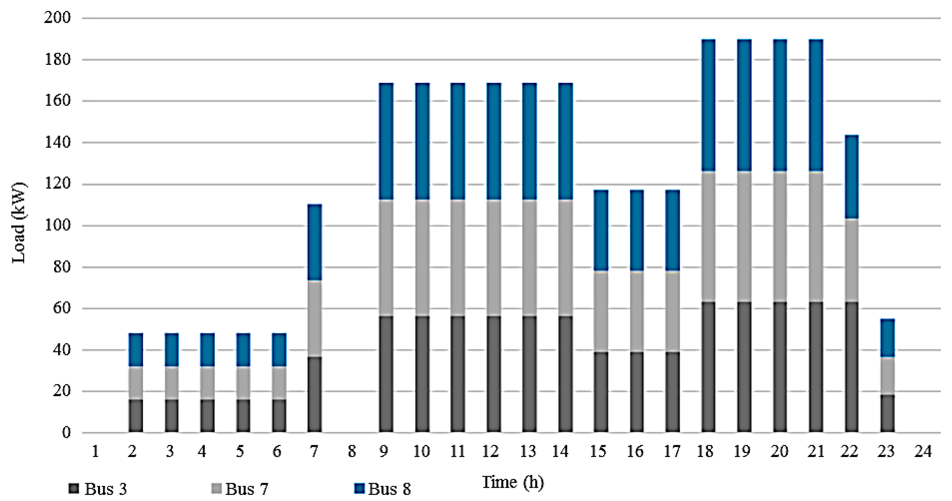
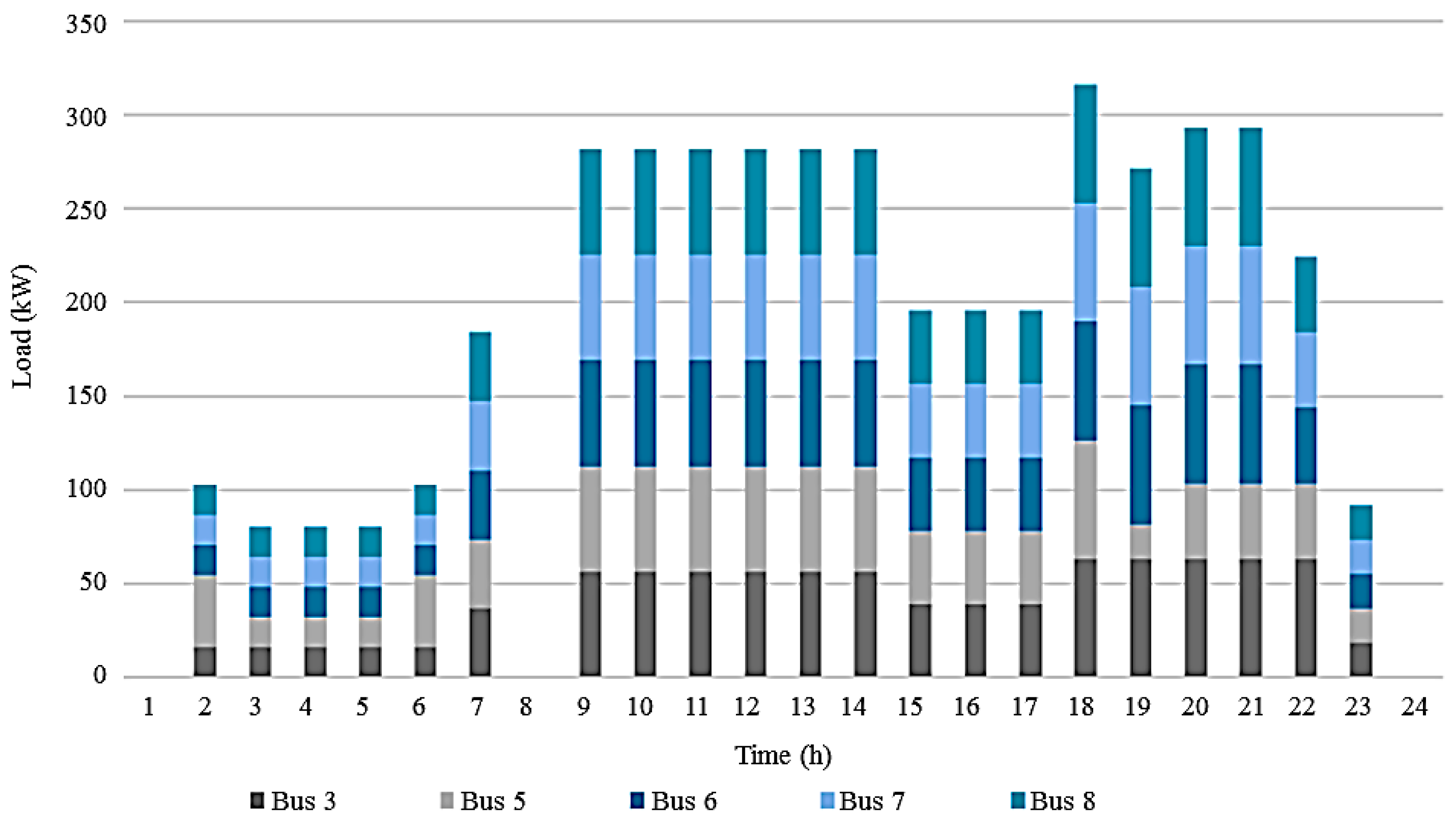
3.3.1. Base Case Comparison with Cases 2 and 3

In this section the base case load profile is compared with the cases where only LC contracts are provided to the consumers (Cases 2 and 3). The consumers using these contracts reduce the load at peak times, namely, from 9:00 to 14:00 and from 18:00 to 22:00. Each DRA contract signed with consumers has a certain amount of load that consumers can reduce. This depends on the period in question (between 18:00 and 22:00 this amount is higher).

In addition, in each contract there is a price associated with the quantity of load transferred, which varies according to the period in question. This price translates to a cost for the DSO. However, from the consumers’ point-of-view, it acts as an incentive in exchange for reducing their load in those periods. Incentive values are proportional to the amount of load offered to consumers.

Figure 8 shows the comparison between the base case and Cases 2 and 3, where DRA are used in three and five buses, respectively. Figure 9 and Figure 10 represent the load that has been reduced at each hour and on each bus for Cases 2 and 3, respectively.

It can be observed the reduced total load in comparison with the base case and it is also possible to notice the differences between Cases 2 and 3. By comparing the peak periods, DRA used in five buses results in a higher demand reduction than when used only in three. For Case 2 there is a reduction of 170 kW between 9:00 and 14:00 and 180 kW during the 18:00 and 22:00, in comparison with the base case.

In Case 3, the mean of reduced load at the various time intervals is about 280 kW, and between 18:00 and 22:00 there is a highest reduction of load. It should be noted that the operational costs of the network, from the DSO point-of-view, is higher in Case 2: In Case 2 the costs are 1053.40 € and in Case 3 the costs are 1037.30 €. In addition, the cost associated with DR in Cases 2 and 3 are 67.80 € and 107.90 €, respectively.

Thus, when DRA are used in five buses, the cost associated with load reduction is higher, compared to the use of DRA in three buses. Hence, it is observed that the decrease in demand is higher when considering DRA in five buses, which makes the load profile more uniform, optimizing the DSM.

3.3.2. Base Case Comparison with Cases 4, 5, and 6

In this section a comparison of the base case is performed with the cases where DRA were implemented in three buses and consumers are offered LS contracts. In Case 4 the prices do not change, which serves as the comparison term for the remaining cases. In turn, in Cases 5 and 6 there is an increase and reduction of the price by 30%, respectively. The LS contracts allow consumers to reduce the load in the peak periods and consequently shift the reduced load to other periods, namely for the valley and off-peak periods.

Thus, the load is shifted from the $T_{tk}^{LS}$ periods (9:00–14:00, 18:00–22:00) to the periods $T_{tk}^{LR}$ (02:00–07:00, 15:00–17:00, and 23:00–00:00). In this way, the LS contracts have different time intervals to which the load can be shifted. In Figure 11, it is observed that in peak periods there is a decrease in demand in Cases 4, 5 and 6 in comparison with the Base-Case. However, this demand increases during the valley and off-peak periods. Thus, it is verified that in these cases there is a load recovery between 02:00 and 07:00, 15:00 and 17:00 and 23:00. In addition, it is observed that when there is a 30% price increase (Case 5 in comparison with Case 4), during the period 02:00 and 08:00 the load profile remains similar. The same happens at 23:00. However, from 09:00 to 14:00 and from 18:00 to 22:00 the demand in Case 4 is 44 kW and 63 kW lower when compared with Case 5, respectively.

This is due to the fact that the contracts with higher prices (Case 5) are associated with higher total operational costs of the grid since the incentives granted to consumers are also higher. Thus, it can be seen that the total cost of the operation and the cost of DR in Case 5 are 1064.90 € and 71.90 €, respectively; while in Case 4 they are 1046.60 € and 90.20 €. In this way, the DSO prefers to choose the contracts that carry a lower cost and to optimize the DSM. Moreover, when there is a reduction of 30% of the price (Case 6), it is verified that (at 02:00, 17:00 and 18:00) there is an increase in demand by 62 kW when compared with Case 4. In the remaining hours the demand remains similar in both cases. In turn, the operational costs and the DR cost in Case 6 are 1016.60 € and 69.90 €, respectively, which are lower values than those obtained in Case 4.

Thus, it is verified that the costs associated with load reduction are higher when contract prices are not modified and lower when they exhibit a 30% reduction. Hence, it is noted that increasing or reducing the price of DR does not substantially influence consumers’ energy demand when DSO considered DRA in three buses. The differences analyzed between the various cases are not significant, since at most a 63 kW oscillation occurred which is a small value to cause an impact on the network. Despite this, the use of DRA in three buses providing LS contracts allows obtaining a more uniform load profile compared to the base case.

3.3.3. Base Case Comparison with Cases 7, 8, and 9

In this section a comparison is made between the base case and the cases which consider DRA in 5 buses. As in the previous section, DRA offers LS contracts to the consumers. The details of these contracts are the same as in the previous section (shown in Table 8). Figure 12 shows a decrease in the demand between 09:00–14:00, and 18:00–22:00 for cases 7, 8 and 9 compared with the base case. Moreover, it is found that between 02:00–07:00; 15:00–17:00; and 23:00–00:00, the demand increases in all of the three cases compared to the base case.

Comparing Cases 7 and 9 with the base case, it is observed that between 09:00–14:00 the load profile is the same for both cases, however, there is a reduction of 280 kW in relative to the base case. Moreover, between 18:00–22:00 the load profile is similar for both cases, since for Case 9 there is an average reduction of 316 kW and for the case 7 it is 280 kW relative to the base case.

During valley hours (from 02:00–19:00) the demand increase is higher in Case 9 than in Case 7 in relative to the base case: in Case 7 it is 157 kW and in case 9 it is 105 kW. At 23:00 the recovered load was the same for both cases (90 kW) relative to the base case. During the off-peak periods (between 15:00–17:00) the load profile is the same for cases 7 and 9, where the load increment is equal to 196 kW, relative to the base case.

Comparing Cases 7 and 8 with the base case, it is verified that between 02:00–06:00 and at 23:00–00:00, the recovered load in these cases is quite similar, being on average 90 kW. However, in Case 7 at 07:00 the recovered load corresponds to 184 kW, while in Case 8 the recovered load is 102 kW. The same happens between 15:00–17:00, where in Cases 7 and 8 the recovered load values are 196 kW and 92 kW, respectively.

Likewise, during the peak periods the load in Case 8 is less reduced when compared with Case 7. Namely, between 09:00–14:00, the difference is 88 kW; while from 18:00–22:00 the average is 120 kW. For all Cases 7, 8, and 9, there is an increase in the demand during the valley and off-peak hours, as well as a decrease in the demand during peak-hours. However, when the DR price increases by 30% the results obtained are not as favorable when comparing Cases 7 and 9 (in-line with the results in the previous section).

It should be noted that Case 9 results correspond to a higher variation of the demand relative to the base case. However, when compared with Case 7, it is observed that the differences between them are significant considering the order of magnitude of the PS grid under study, i.e., at maximum of 50 kW oscillation occurs between the load profiles of both cases. The differences between Cases 7 and 8 are more significant, since in peak periods there is a variation of values higher than 100 kW.

When comparing the operational costs of the grid (shown in Table 5), it is observed that the base case presents a cost of 1014.30 €, while in Cases 7, 8 and 9 these same costs are 1023.50 €, 1055.70 €, and 977.50 €, respectively. Thus, it is observed that when contract prices are reduced by 30%, the operations costs are lower than those of the base case. Moreover, in Cases 7 and 8 the operating costs are higher than the base case. However, both cases are favorable to the DSO relative to the base case, since DSO is enhancing the DSM either way. It should be noted that the higher the incentives given to consumers, the higher is the grid operating costs from the DSO point-of-view. The DR costs for Cases 7, 8, and 9 are 146.80 €, 105.70 €, and 117.70 €, respectively. Thus, when there is no change in the contract prices, these costs are higher than in other cases.

This happens, since in Case 8, with the increase of the incentives, the load reduction is not so significant, so the DR cost is lower than the other cases. In Case 9 when the prices are reduced by 30%, the associated cost is also lower. However, this case is characterized by the high reduction of load, which does not allow the DR cost to be lower than that of Case 8. It is noted that the use of DRA in five buses allows a more uniform load profile compared with the base case in addition as reducing the operating costs, increasing the flexibility of the PS.

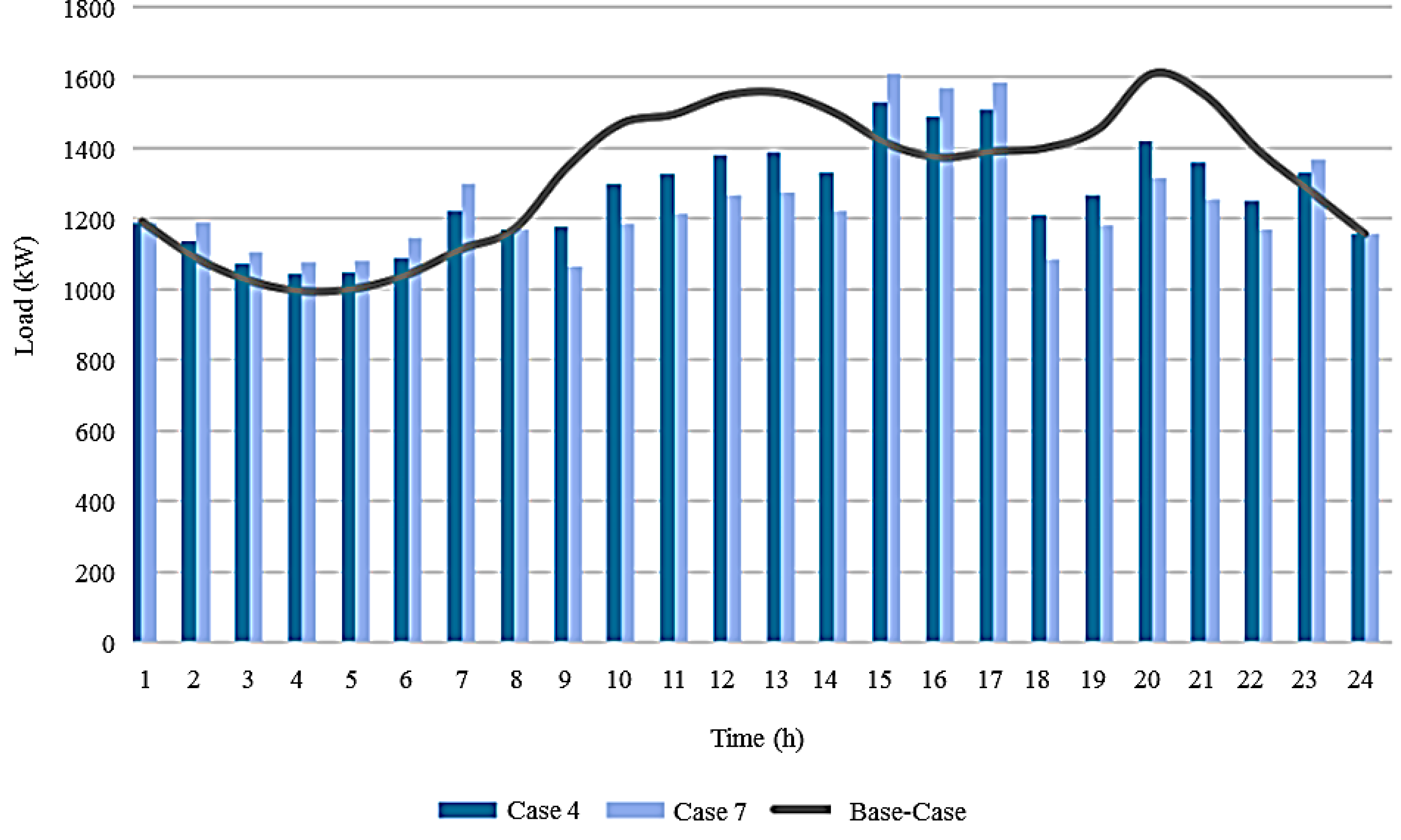
3.3.4. Comparison between Case 4 and Case 7

In this section a comparison is made between Cases 4 and 7 in order to verify the differences between having DRA in three or in five buses, considering the cases whose contracts do not present changes in their prices. In Figure 13 it is possible to verify that, when DRA is used in the five buses, during the peak hours, a higher reduction of the demand is observed in comparison with the case where three buses are considered.

Between 09:00–14:00 there is a load difference of 115 kW and between 08:00-22:00 the load difference is 100 kW. During the valley periods the difference is not significant, since in Case 7 there is an increase of 46 kW of recovered load compared with Case 4. During off-peak periods, namely between 15:00–17:00, the load value is 79 kW.

The recovered and reduced load on each bus for Cases 4 and 7 are shown in Figure 14 and Figure 15, respectively. From the figures it is possible to verify the influence of each bus on the energy demand. Also, it is possible to observe the total reduced load and recovered load relative to the base case in each hour. It is verified that the relevance of the various buses in the modified load profile is similar for each hour.

The differences between the presence of DRA in three or five buses are only significant during the peak-hours. In addition, from Table 5 it is verified that when DRA is used in five buses, the total operation cost is 1023.50 € and the DR cost is 146.80 €, while when considering the DRA in three buses the operating cost is 1046.50 € and DR cost is 90.20 €.

In this way, is verified that when considering aggregators in more buses it is possible to reduce the operational costs of the grid under study, even when the associated cost with the load reduction is higher.

4. Conclusions

In this work, a distribution system management model was proposed in the form of a two-stage stochastic problem with the integration of RES (wind and PV power) in order to deal with associated uncertainties (10 different scenarios were modeled for each RES). The proposed model considers DSM in order to increase the flexibility of the PS and the various scenarios of RES production were modeled as stochastic parameters. Several DRA integration options were considered which provide different types of DR options to consumers (LC, LS, and LR). The proposed model was tested using a distribution grid with 15 buses. Nine case studies were modeled considering different levels of DRA integration (i.e., in three and five buses), DR options, and contract prices (variation of ±30%).

The results obtained show that when DRA offer LC contracts to consumers, there is a reduction in demand during peak-hours. However, when LS contracts are provided, in addition to peak demand reduction, there is an increase in load recovered during valley and off-peak hours, resulting from the LR option. Thus, the LS strategy allows obtaining a more uniform load profile compared to the LC option. When comparing the cases where DRA are present in three vs. five buses (regardless of variations in DR prices), it is observed that with DRA in five buses the optimization of DSM is more significant since DSO operation costs are lower.

When DR prices sold to consumers have a 30% of reduction, a higher reduction in peak-hours demand and an increase in recovered load during the valley and off-peak hours were observed compared to cases where prices remain unchanged. Moreover, when the prices increase by 30%, DSM is not as effective compared with other cases.

This is because the use of higher incentives translates into higher operating costs, and vice versa. Therefore, the DSO selects the contracts that carry a lower cost and consequently allows the improvement of the PS flexibility. It should be noted that DR prices variations when DRA are present in three buses, are not significant compared to when DRA are considered in five buses. In addition, in the various case studies, the operating costs were higher than the base case (no DR) except in the case with DRA in five buses and 30% in the incentives reduction.

However, although the operational costs of almost all cases studies are higher than the base case, even such differences are not significant. DRA are shown to have benefits for the DSO, since they guarantee the demand-side optimization, increasing the PS reliability and efficiency. Finally, the incorporation of DRA in the PS, together with RES integration as considered in this study, ensures efficient DSM where consumers play an active role in the system. The demand is adapted to be supplied, system flexibility increases, total operation costs from the DSO point-of-view can be minimized, and electricity costs for the consumers are reduced.

For future remarks more studies should be conducted considering the internet of thing concepts together with further analysis around the concept of transactive energy. Such concepts may increase the benefits and strategies between householders, DSO and retailers, flattening the load profile.