A Holistic Review on Biomass Gasification Modified Equilibrium Models


1
CT2M—Centre for Mechanical and Materials Technologies, Mechanical Engineering Department of Minho University, 4804-533 Guimarães, Portugal
2
VALORIZA-Research Center for Endogenous Resource Valorisation, Polytechnic Institute of Portalegre, 7300-555 Portalegre, Portugal
3
CIENER-LAETA/Faculty of Engineering, University of Porto, 4200-465 Porto, Portugal
*
Author to whom correspondence should be addressed.
Energies 2019, 12(1), 160; https://doi.org/10.3390/en12010160
Submission received: 2 December 2018
/
Revised: 24 December 2018
/
Accepted: 26 December 2018
/
Published: 3 January 2019
(This article belongs to the Collection Bioenergy and Biofuel)
Abstract
:Biomass gasification is realized as a settled process to produce energy in a sustainable form, between all the biomass-based energy generation routes. Consequently, there are a renewed interest in biomass gasification promoting the research of different mathematical models to enlighten and comprehend gasification process complexities. This review is focused on the thermodynamic equilibrium models, which is the class of models that seems to be more developed. It is verified that the review articles available in the literature do not address non-stoichiometric methods, as well as an ambiguous categorization of stoichiometric and non-stoichiometric methods. Therefore, the main purpose of this article is to review the non-stoichiometric equilibrium models and categorize them, and review the different stoichiometric equilibrium model’s categorization available in the literature. The modeling procedures adopted for the different modeling categories are compared. Conclusion can be drawn that almost all equilibrium models are modified by the inclusion of empirical correction factors that improves the model prediction capabilities but with loss of generality.
1. Introduction
Gasification occupies a preponderant position from both economic and efficiency perspectives [1]. It is considered an important route to convert biomass and waste materials into useful gas products that can be converted into energy by several technological options—boilers, engines, turbines and fuel cells—or used as raw material to produce value-added fuels, hydrogen gas or chemicals [2,3].
Some technological problems remain unresolved in gasification for a robust market penetration [4]. The main challenge is related with the optimization and understanding of the reactor behavior, which is the lowest efficiency component of a gasification plant [5]. Its design and operation encompass the comprehensive knowledge of the gasification process and how the design, biomass, and the operating parameters influence the overall performance [6].
Another challenge is the development of gas cleaning systems in an efficient and cost-effective way for downstream application of biomass gasification technology for power, biofuels and chemicals production [7,8]. Gas cleaning must be applied to prevent erosion, corrosion and environmental problems in downstream application [7]. Tars are mostly heavy hydrocarbons resulting from a biomass gasification process that can block engine valves or cause fouling of a turbine leading to higher maintenance costs and lower performance. In addition, tars interfere with the synthesis of fuels and chemicals [8,9].
The development and implementation of mathematical models is essential to understand and predict the process behavior and to analyze effects of different variables on the process performance.
These numerical models have also the advantage of avoiding the high experimenting costs and allow us to study different scenarios with different levels of complexity, avoiding time consuming and costly procedures [10].
It is not surprising that different types of models have been developed over the years, from complex three-dimensional models, to the simplest zero-dimensional models. Models have been published using different classifications, designations and categories. The most general classification of the gasification models is: thermodynamic equilibrium, kinetic, computational fluid dynamics (CFD) and artificial neural networks (ANN) [6]. Although there are variations on the modeling approaches, one can conclude from the literature that the above classification is well accepted by the scientific community [11,12,13,14].
Mathematical modeling is usually founded on the laws of mass, energy and momentum conservation. Fluid dynamics and chemical reactions are taken into consideration in more complex models. The simplest models consider mass and energy balances throughout all the reactor to predict the composition of the produced gas, not considering particular processes and chemical reactions. They consist of global mass and heat balances of the entire reactor and are named equilibrium models. For equilibrium modeling, one may use stoichiometric or non-stoichiometric methods [12,13,14]. The mathematical model used in the stoichiometric method includes a set of chemical reactions for which the equilibrium constants are defined. Contrarily, in the non-stoichiometric method, there is no need of knowing the reaction mechanism to resolve the problem. The equilibrium condition is attained by minimization of Gibbs free energy. This method needs only as input, the elemental composition of the feedstock. Therefore, this method is mostly appropriate for biomasses, which the chemical formula is not evident but can be obtained from ultimate analysis [6].
Kinetic models are typically used to describe kinetic mechanisms of the thermal pyrolysis and gasification. In these models the various chemical reactions and transfer phenomena between phases are considered [15,16,17]. The kinetic models are able to predict the produced gas composition, temperature and the overall reactor efficiency. The kinetic models are more appropriate and precise at relatively low operating temperatures due to required long residence time for complete conversion [18]. The kinetic models are a powerful and more accurate tool in the investigation of the gasifier behavior, but they also need more computational resources [19].
A CFD model offers the study and analysis of fluid flow, heat transfer, mass transfer, chemical reaction and related phenomena systems solving a set of mathematical equations that describe these processes and using numerical methods in computer-based simulations [20]. In a gasification scenario, the CFD model usually includes various sub-models related to the biomass particle such as vaporization, pyrolysis, secondary pyrolysis, and char oxidation [6,21]. Other advances have been achieved like the fragmentation of fuels during gasification and combustion [22]. This refined approach is generally accomplished using commercial software, which have been practiced by several authors [23,24,25,26,27]. In order to explore the several geometries and operating conditions of a reactor CFD is seen as an economical option to investigate the ideal configuration considering the project specifications. In the CFD model the fluid mechanics is treated in detail, and this is the crucial distinction when CFD is compared with the other kind of models [11].
ANN models use a pure mathematical modeling approach that correlates input and output data to create a mathematical prediction model. An ANN model imitates the working of the human brain to process information fast and efficiently through a system of neural networks given to the model some human characteristics. The use of ANN models for biomass gasification are very limited [28], being the signal processing and function approximation its main applications [14]. Input data sets are the only inlet required in ANN. No mathematical description of the process is necessary, so they are more appropriated for scaling-up and simulation of a process. Consequently, it can be considered that ANN are not a feasible option for biomass gasification due to the restricted number of experimental data available [14].
From the above exposition, the selection of the most appropriate model to a given application depends on the goals defined and the experimental data available. Sophisticated models are more useful, because they allow obtaining more information on the process. However, this option is dependent upon the availability of reliable input data. Otherwise, simpler models may be more appropriate for certain applications as long as their limitations are known. In certain cases, such as preliminary studies, constrained equilibrium models are sufficient.
This review is focused on the modified equilibrium models specially in the non-stoichiometric method where the review literature is inexistent. A problem that arises from these modified equilibrium models is that they are receiving several different designations that are needed to be clarified. The following subsections depict the opportunity and a justification for this review.
1.1. Existing Reviews
There are various relevant reviews on modeling of biomass gasification, mostly recently [11,12,13,14,15,22,29]. The majority of this literature is focus on all categories of models [11,12,13,14]. Other available reviews are oriented towards fixed [15] or fluidized beds [11,15,22]. As far as thermodynamic equilibrium modeling is concerned, the literature is very scarce, being the recent review of Villetta et al. [29] with a focus in the stoichiometric method the sole example. Table 1 summarizes the existing reviews on biomass gasification models and their objectives.
Gómez-Barea and Leckner [11] review the biomass fluidized bed gasification modeling. Bubbling and circulating fluidized beds modeling are discussed with focus on comprehensive fluidization models. The work emphasizes the prediction of the bubbling fluidized bed gasification models in terms of gas composition, solid conversion and gasification efficiency. It is also reviewed the main CFD tools applied to biomass gasification in fluidized beds. The equilibrium models are categorized as black-box or zero-dimension models. The designation black-box model comes from the fact that the processes inside the reactor are not determined. In the black-box models the authors includes the simple mass and heat balances; the equilibrium models; pseudo-equilibrium models, that are modified equilibrium models supplemented by empirical correlations; zone models, that divide the gasifier into black-box regions; empirical or fitting-data models, that use empirical correlations obtained from fitting experimental data in a specific reactor.
From these different equilibrium model types, it is possible to verify the great variety of equilibrium models that have been developed. The first type of models consists of overall mass (species) and heat balances over the entire gasifier supported by assumptions to determine the material distribution in the reactor. This type of models does not include the equilibrium relationships and hence are out of the scope of the present review. Equilibrium models and equilibrium models enhanced by empirical correlations obtained from experimental data, classified by the authors as pseudo-equilibrium models, will be the main focus of the present review. However, the designation pseudo-equilibrium models should rather fall into the modified equilibrium model’s category in order to avoid possible misunderstandings with the thermodynamic pseudo-equilibrium process. In the so-called zone models, the reactor is divided into black-box zones where different gasification phases are considered and different models can be used. This type of models is still an equilibrium model; therefore, it should also fall in the modified equilibrium model category. Finally, other researchers simply use empirical correlations to improve the model predictions of specific gasifiers. These models are classified by Gómez-Barea and Leckner [11] as empirical or fitting-data models. This class of models is similar to the pseudo-equilibrium models only differ in the amount of data considered. Therefore, it should also be included into the category of modified equilibrium models.
Puig-Arnavat et al. [12] divided the models into thermodynamic equilibrium, kinetic rate, and ANN models. Regarding the thermodynamic equilibrium models, they identified two classic methods - stoichiometric and non-stoichiometric. All the equilibrium models departing from these two classical approaches are refereed as modified and corrected equilibrium models. Equilibrium models are founded on common assumptions suitable for some types of reactors for which equilibrium models have better predictive capabilities. Owing to these assumptions, equilibrium models have wide divergence under specific conditions. Common drawbacks at relatively low temperatures are the overestimation of hydrogen and carbon monoxide yields and the underestimation of carbon dioxide, methane, tars and char. For these reasons, numerous researchers have developed modified equilibrium models or used the quasi-equilibrium temperature approach. Besides the excellent description of the equilibrium models, the mathematical formulation is not shown and the intensive development of equilibrium models in the literature are not classified.
Baruah and Baruah [13] categorized the approaches for gasification modeling into thermodynamic equilibrium, kinetic and ANN. They reviewed the biomass gasification modeling approaches classifying the thermodynamic equilibrium models as thermodynamic models, modified thermodynamic models or thermodynamic models incorporating empirical parameters. Equilibrium models are additionally categorized as stoichiometric and non-stoichiometric models. Besides the effort to categorize the recent equilibrium modeling works, the mathematical formulation is not shown.
Loha et al. [22] investigated different modeling approaches classified as follows: equilibrium models, rate based or kinetic models and fluid dynamics. Regarding the equilibrium models they are subcategorized into stoichiometric and non-stoichiometric equilibrium models. The equilibrium models including different improvements towards better agreement against experimental data are referred as modified equilibrium models. Mathematical formulations for fluidized bed gasification was discussed, as well as their merits and demerits. A detailed review of different models used by different researchers and the main results obtained are presented, whereas a special focus is given to CFD models.
Patra and Sheth [14] discuss different modeling approaches for downdraft gasifiers. The models were divided into equilibrium, combined transport and kinetic, CFD, ANN and ASPEN Plus models. Regarding the equilibrium models they are also further subcategorized as stoichiometric and non-stoichiometric models. Although, the review is oriented to the downdraft gasifiers a general mathematical formulation of the equilibrium model is given. This approach is independent of the gasifier geometry; hence it can be applied to other reactors. When reviewing the equilibrium models, they implicitly recognize the existence of another category of equilibrium models that are referred as modified models. However, the formulation of these modified models is not explicitly shown and a formal categorization of the equilibrium models is also missing.
Recently, Villetta et al. [29] reviewed the gasification models highlighting those based on the stoichiometric method. They considered stoichiometric models as an evaluation of the equilibrium constants for an independent set of reactions, which may also be associated with Gibbs free energy. Non-stoichiometric modeling approach is presented as a developed based on the direct minimization of the Gibbs free energy of reaction, therefore it is also referred as “Gibbs free energy minimization approach”. Detailed mathematical formulation for the stoichiometric equilibrium model is presented and several developed models of this category are described. However, the non-stoichiometric model description is not on the scope of their review.
1.2. Motivation and Objective of the Review
The aim of this work is to review the biomass gasification modified equilibrium models with emphasis on the non-stoichiometric method and on the categorization of both equilibrium modeling approaches. Comparisons are made of the modeling procedures for each model category.
The inclusion of the equilibrium modeling approaches categorization is crucial and is motivated by the several examples found in the scientific literature showing different and somewhat hermetic designations of the developed model that needs clarification. For example, Kangas et al. [30] perform a categorization of the equilibrium models as shown in Table 2.
Kangas et al. [30] categorize the equilibrium models into four categories: equilibrium, modified equilibrium, quasi-temperature and constrained free energy. From the description of the models, it is possible to determine that the first category (thermodynamic equilibrium) is in the reality the pure equilibrium approach being the other three categories all modified equilibrium models. The modified equilibrium models are defined as an extended thermodynamic equilibrium model by dividing the model in two parts. One part of the gasified biomass bypasses the equilibrium reactor and is converted into tar, char and light hydrocarbons. The other part of the biomass is modeled using thermodynamic equilibrium.
In the quasi-temperature model approach, the reaction temperature is lowered to estimate the formation of light hydrocarbons, tars and char. The constrained free energy method is an upgrading to Gibbs free energy method by introducing additional immaterial constraints. As the additional constraints are related to physical entities without material content such as extent of reaction, electrochemical potential and surface area or volume, they have been designated as immaterial [31]. The distinct advantage of this method is settled in the calculation of constrained chemical reactions, state properties and enthalpic effects simultaneous and interdependently.
Vakalis et al. [32] presented a multi-stage and two-phase thermodynamic gasification model. This model was designated as multi-box model. The basic idea of the multi-box model is to improve the black-box thermodynamic model (or single stage model) by developing multiple transitional boxes that compute two phase (solid-gas) equilibrium. Biagini et al. [33] developed a so-called bi-equilibrium model for biomass gasification in a downdraft reactor. According to the authors this multizonal model is based on non-stoichiometric equilibrium modeling features. Lim and Lee [34] presented a so-called quasi-equilibrium thermodynamic model for biomass gasification. This designation of the model was advanced solely based on the introduction of empirical factors preventing the model to reach the equilibrium.
From the previous paragraphs it is possible to verify that there are different approaches with several designations and classifications for the thermodynamic models. Apparently, some entropy can be generated with so many designations and classifications. The main purpose of this paper is to review the modified thermodynamic equilibrium models used in biomass gasification and elucidate about the designations, there complexity and the different assumptions.
2. Gasification Process
Gasification is a thermochemical conversion process at high temperatures involving partial oxidation of the fuel components [6,35]. From the gasification process a fuel gas is obtained (synthesis gas or syngas), which composition depends on various factors such as the type of biomass, reactor design and operational conditions (temperature, pressure and gasifying agent) [36].
The produced gas is a mixture of carbon monoxide, carbon dioxide, methane, hydrogen, water vapor, nitrogen and light hydrocarbons, such as propane and ethane, and heavy hydrocarbons, such as tars [35,36]. Small amounts of hydrochloric acid (HCl) and hydrogen sulfide (H2S) can also be found in the produced gas [37]. Gasification takes place in four phases: drying, pyrolysis, oxidation and reduction that can be described as follows [38,39]:
- Drying—where moisture is transformed into steam at temperatures around 100–200 °C. At these temperatures no chemical reaction takes place; the biomass is not decomposed. For a produced gas with high calorific value, the vast majority of gasification systems use biomass with moisture content in-between 10 to 20%;
- Pyrolysis—is the thermal decomposition (devolatilization) of the dry biomass in the absence of oxygen at temperatures in-between 150–700 °C releasing the volatiles components and a residue containing char and ash. The volatiles produced are a mixture comprising mostly carbon monoxide, hydrogen, carbon dioxide, light hydrocarbons, tar (liquid fraction) and water vapor;
- Oxidation—various oxidation chemical reactions take place in a gasification scenario releasing the heat needed for the endothermic reactions. The reaction between the char and oxygen, forming carbon dioxide. The hydrogen in the biomass is oxidized to generate water. The oxygen is present in sub-stoichiometric amounts; partial oxidation of carbon might occur, resulting in the production of carbon monoxide;
- Reduction—various chemical reactions mainly endothermic occur without the presence of oxygen due to its consumption in the oxidation reactions. The main products of the reduction reactions are hydrogen, carbon monoxide and methane.
Although these steps are often described and modeled in series as depicted in Figure 1, in a real gasification scenario there is no clear boundary between them and they often occur simultaneously.
In a biomass gasification scenario, the biomass is primary dried and then it experiences thermal degradation in the pyrolysis step. Pyrolysis products can react between themselves, as well as with the gasifying agent, to form the ultimate gasification products. The char produced is a product containing unconverted carbon, some hydrocarbons and ash [37]. While the quantity of char largely depends on the reactor and operational conditions, the amount of ash depends on the biomass used.
The following list shows the most relevant chemical reactions that occur in a gasification process:
Carbon Reactions
Boudouard:
Water-gas or steam
Hydrogasification
Oxidation Reactions
Shift Reaction
Methanation Reactions
Steam Reforming Reactions
As is possible to verify, the gasification process is globally endothermic being the required heat obtained by two possible ways. When the heat required is produced outside the reactor, gasification is called allothermal (or indirect). When the heat is produced inside the reactor due to exothermic reactions, gasification is called autothermal (or direct) [40].
3. Gasification Equilibrium Models
At chemical equilibrium conditions, a reacting system is at its most stable composition, a condition achieved maximizing the entropy and minimizing the Gibbs free energy. As we have seen previously, there are several approaches to model the gasification processes, being equilibrium modeling one of them. There are two general approaches for equilibrium modeling: stoichiometric equilibrium model (based on the equilibrium constants of gasification reactions) and non-stoichiometric equilibrium model (based on the minimization of the Gibbs free energy) [12,13,14,22,29].
The chemical reactions and species involved in the model are required for the stoichiometric approach whereas the non-stoichiometric method is based on Gibbs free energy minimization [6,12,29]. Smith and Missen [41] shown that these approaches are essentially equivalent, and that is corroborated by others authors that considered both approaches conceptually similar [42,43]. The stoichiometric approach might also employ free energy data to determine the equilibrium constants of a predefined set of reactions [12,44].
The main equilibrium models available in the literature considers several simplifying assumptions that are comprehensively resumed by Villetta et al. [29]:
- Steady state;
- Reactions reach the equilibrium state (infinite residence time);
- Homogeneous mixing with uniform pressure and temperature;
- Kinetic and potential energies are neglected;
- Perfect gas behavior of the gas phase;
- Pyrolysis is considered a single step reaction producing gas, tar and char;
- Gasifying medium is enough to convert all carbon of the biomass;
- The gasifier operates at constant pressure and temperature;
- The reactor is considered adiabatic;
- The produced gas does not contain oxygen;
- Nitrogen is considered as inert;
- Solely major species compose the produced gas (CO, H2, CO2, CH4, N2 and H2O);
- Tar is not modeled or modeled in the gas phase;
- Ashes are not considered in energy balances.
Due to the above assumptions, pure equilibrium models yield large divergences under certain conditions. Characteristic drawbacks at relatively low temperatures are the overestimation of hydrogen and carbon monoxide yields and the underestimation of carbon dioxide, methane, char and tar [45].
When developing a gasification model, the first step is the definition of a system of equations representing the gasification process. The number of equations is defined as a function of the number of unknowns. In the side of the reactants the unknown is only the oxidant, while in the products side there are only unknowns [46].
In the following subsections, different approaches and conditions for stoichiometric and non-stoichiometric equilibrium will be presented concerning the definition of the system of equations, which generally are all developed based on a global gasification reaction.
3.1. Stoichiometric Modeling
As mentioned before, in the stoichiometric method, the algorithm that predicts the gas composition is subjected to chemical equilibrium among the different species. To discuss this matter, the gasification process of a mole of biomass in m moles of air can be represented by the following global gasification reaction:
where n1 to n6 are the stoichiometric coefficients. CHxOyNz represents the biomass feed material and x, y, and z represent numbers of atoms of hydrogen, oxygen, and nitrogen per number of atoms of carbon present in the biomass and w, is molar moisture amount in the biomass. All these quantities can be obtained from the ultimate analysis. It is possible to find several modeling studies in the literature where the global gasification reaction includes other terms as will be seen in the next section.
The material balance equations for C, H, O and N are presented below:
The next step in the model formulation is the equilibrium constants definition. In this step special care must be taking in order to select independent chemical reactions [6,47]. From the computational point of view, the independence concept is relevant. If there is a non-independent group of reactions the model will be computing repeated information. This happens when a reactions group can be written as a combination of at least two of the others. The most important gasification reactions to determine independent combinations are the Boudouard reaction (Equation (1)), the endothermic water-gas (Equation (2)), the exothermic methane formation (Equation (3)), the water-gas shift reaction (Equation (9)) and methane reforming reaction (Equation (11)). There are ten possible combinations, eight combinations are independent and two dependents, specifically the combinations of Equations (1), (2) and (9) and Equations (2), (3) and (11). Two independent equilibrium reactions are sufficient to model the gasification process, for example Equations (3) and (9) (methanation and water gas reactions); the equilibrium constants for those gasification reactions are:
These two sets of equations (mass balance and equilibrium constants) can be solved simultaneously to obtain the composition of produced gas at steady state. Resolving the equations system (16)–(21) we find six unknowns (n1 through n6), allowing to obtain the composition and yield of the produced gas for a given equivalence ratio.
The following step is the energy balance given by Equation (22) from which the gasification temperature can be obtained considering that the process is adiabatic:
Thus, and considering the biomass reaction with air, Equations (15) and (22) can be expressed as:
Since , are zero at ambient temperature, Equation (23) reduces to:
, and represent the biomass enthalpy of formation for the different chemical species, the enthalpy of vaporization of water, and the specific heat, respectively. refers to the temperature difference between the gasification temperature and the biomass feed temperature.
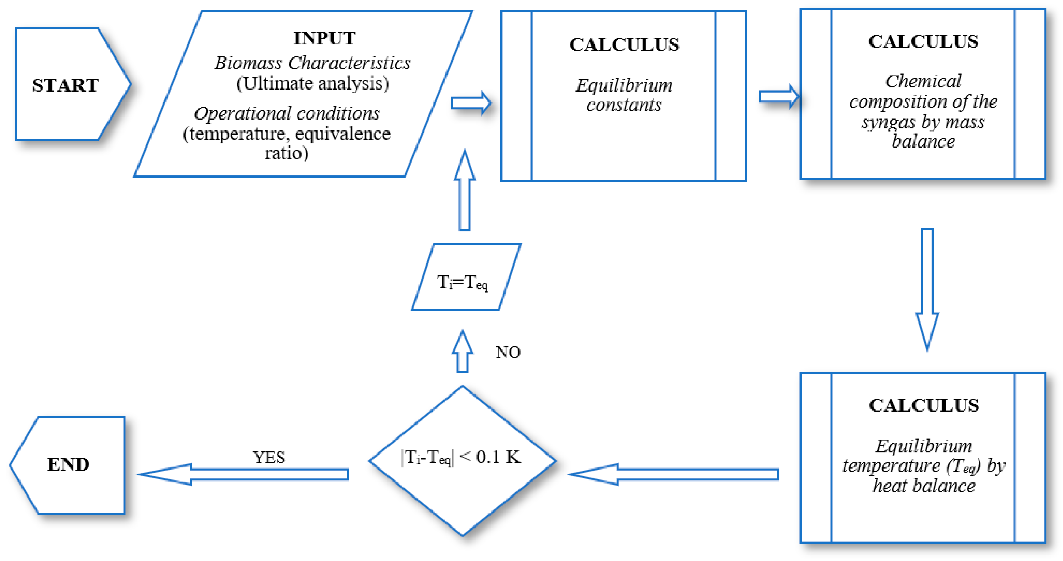
The system of equations is general solved using the iterative Newton-Raphson method, although other possibilities are available. The flowchart of a stoichiometric equilibrium model is shown in Figure 2.
3.2. Non-Stoichiometric Modeling
The non-stoichiometric equilibrium modeling method involves the minimization of the Gibbs free energy of the system [6,12]. This approach is termed non-stoichiometric due to the absence of any specific chemical reaction, other than the assumed global gasification reaction. Therefore, there is only one input required, the elemental composition, obtainable by ultimate analysis. For this reason, non-stoichiometric models are particularly suitable for cases in which all the possible reactions that can occur in the system are not fully known as is the case of gasification. As these methods are based on atom balance of reactants, particular cases like biomass, with unknown molecular formula can also be handled.
The Gibbs free energy, Gtotal, of the gasification product involving N species (i = 1, …, N) is given by:
is the standard Gibs free energy of formation of species i, at the normal pressure. Equation (25) must be solved for the ni unknown values to minimize Gtotal, keeping in mind that it is subject to the overall mass balance of the individual elements. For each element j, we can write:
Aj is defined as the total number of atoms of the jth element reaction mixture, ai,j is the number of atoms of the jt,h element in a mole of the it,h species.
Notwithstanding existing several possibilities to minimize the Gibbs free energy, the Lagrange multipliers yield satisfactory results [44,48], hence consider here. Other alternatives will be discussed in the next section.
The Lagrangian function (L) is formed through the Lagrange multipliers λj = λ1, …, λk, and can be defined as:
Dividing Equation (27) by RT and setting the partial derivatives equal to zero, we find the extreme point.
Finally, replacing the value of Gtotal from Equation (25) in Equation (27) and taking its partial derivatives the Gibbs free energy can be expressed as follows:
Equation (29) can be formed in terms of a matrix with i rows and can be solved simultaneously by some iteration technique.
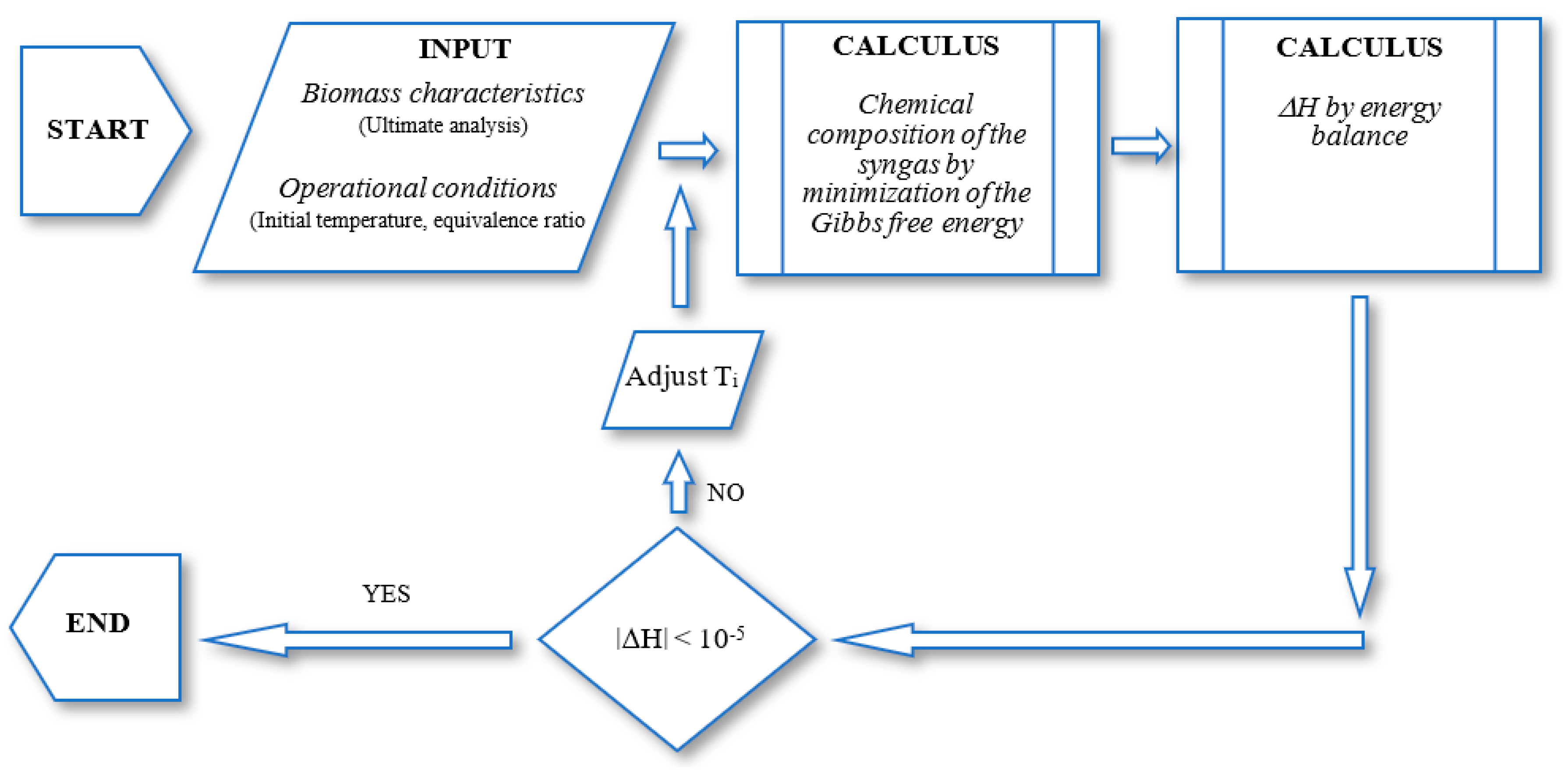
As in the stoichiometric equilibrium models, several approaches/modifications can be found to non-stoichiometric equilibrium models. These approaches and modifications will be comprehensively described in the next section. The algorithm shown in the Figure 3 requires the assignment of a process temperature. Therefore, in the first iteration, an initial guess for the temperature is established and used to estimate the gas composition.
4. Modified Equilibrium Models
Thermodynamic equilibrium models are often assumed to be a guideline, especially for high temperatures (more than 800 °C), being useful for several engineering applications predicting the maximum conversion obtained for a given reaction condition. However, equilibrium conditions may not be reached in practice at low temperatures (less than 800 °C). Several authors report that thermodynamic results deviate from experimental data due to the presence of non-equilibrium factors in the reactor.
It is frequently pointed out the underestimation of CH4 and CO2 and the overestimation of CO and H2 in the gas produced [30,45]. It is also reported that during biomass gasification also tar, char, ammonia and light hydrocarbons can be formed [49,50,51]. Those deviates take us into the discussion of the different approaches of the equilibrium models that tends towards the minimization of those limitations. The most pertinent equilibrium models are described in the next subsections respecting the chronological order of appearance.
4.1. Stoichiometric Method
Table 3 shows the most relevant equilibrium models in a chronological order in order to demonstrate the evolution and the trend of the modeling approaches. The list is not exhaustive but long enough to draw conclusions on techniques that are being used.
Only the main aspects of the models are shown, such as the global gasification reaction, the equilibrium conditions, and other specific features such as the treatment of the tar, char and ash. From Table 3 it is possible to inquire that many efforts were applied since the work of Zainal et al. [46] with the objective of approximate the simulated syngas composition to the experimental measured syngas composition. It is also possible to conclude that the pure equilibrium models were abandoned being all modified in some sort of features.
The predicting capabilities of the models were not directly included in Table 3 in order to keep it with reasonable dimensions. Nevertheless, the predicting capabilities of the different models are indicated by the products of the global gasification reaction as well as the temperature needed for the heat balance. There are different approaches to modify the pure equilibrium models in order to improve their prediction capabilities. The most common is the use of correction factors that are multiplied by equilibrium constants for the reactions (most common: methane formation, homogeneous water-gas reaction, and methane reforming) used in modeling of syngas composition. The simplest correction factors are calculated in an empirical manner (attempt and error) on different researches regarding modeling of syngas composition for a specific reactor type, which does not allow the general use for other type of gasifiers. Although the modifications increase the accuracy of the model predictions, the lack of a correlation with the gasification conditions makes these models less reliable. The more sophisticated correction factors use computer algorithms for the error minimization and are generally more complex than a simple constant. In this regard, these correction factors may assume different forms since a simple constant [42,62,66,67,70] to a more or less complex functions of equivalence ratio [34,65,71,74], gasification temperature [63,74] and equilibrium temperature [68,74].
Other approaches have been made such as the use of the carbon boundary temperature [53,62,67]. The carbon boundary temperature (or carbon boundary point, as is also known) is the temperature obtained when exactly enough gasifying agent is supplied to attain complete gasification. This approach is also considered as a two-stage model being the first stage below the carbon boundary temperature, where only heterogeneous reactions occurs, and a second stage, where only homogeneous reactions take place. The main advantage of using the carbon boundary point is the fact it represents the optimal conditions for gasification considering both the energy and exergy efficiencies as was demonstrated by Desrosiers [75], Double and Bridgwater [76] and Prins et al. [77]. Energy and exergy in the syngas have a pronounced maximum at the carbon boundary point. That is the reason why the gasification parameters at the carbon boundary point are considered the ideal conditions for a gasifier to operate [77].
Approaches that are more sophisticated are also being implemented such as the three-stage model of Ngo et al. [63]. The idea of dividing the model into three stages is based on the fact of pyrolysis is the most significant step of biomass gasification, since it remarkably influences the final produced gas composition [78,79]. Therefore, a detailed knowledge of devolatilization is crucial for an accurate prediction of the model.
The mathematical modeling of the gasification departs from a proposed global reaction. On the reactants side the biomass is usually represented by a molecule comprising C, H, O and N [34,42,59,62,66,67,71,72]. Some authors consider also sulfur (S) in the biomass molecule [55,56,58,68,71], and others neglected the nitrogen content in the biomass molecule [46,52,53,65,74]. Biomass moisture is usually represented by a specific term in the global gasification equation. The main gasifying agents used in the modeling works are air, air and steam [64,65,66,71], just steam [63], oxygen and steam [54] and oxygen enriched air [67].
Considering the side of the products, the principal species presented in syngas are H2, CH4, CO, CO2, H2O, and N2. These six gases leaving the gasifier are considered by few authors [37,41]. In addition, the unconverted carbon (C) is included by several authors [34,52,56,58,62,65,69,70,71,74]. Instead, some authors consider tars [59,66], others char [63,67], tar and char [72] and ashes [68]. Other gases can also be found, such as H2S [58], SO2 [55,56,68] as resulting products of the inclusion of the sulfur in the biomass molecule.
The particular case of the ashes comprising chemical compounds such as SiO2, CaO, Al2O3, MgO, KO2, among others [47], are neglected in the major part of the modeling studies. The ash present in the biomass is considered as inert in the modeling studies or chemically represented solely as SiO2 [68], due to its higher content in many biomass ashes [47].
Tar is an unwanted product of biomass gasification due to the various problems of slugging and fouling in the downstream equipment [79]. Although there are hundreds of species in a tar sample it is commonly treated by the single major component benzene (C6H6) [80,81]. This is the case of model studies [59,70,71,73], but other possibilities are also being used such as a tar molecule of CH1.003O0.33 implemented by Barman et al. [66], or a tar molecule of C6H6.2O0.2 implemented by Gagliano et al. [72]. Various correlations for tar yield are implemented assuming different forms since a simple mass percentage [72] to complex temperature functions [59,70,71].
In a real biomass gasification scenario, the carbon conversion is not possible to completely accomplish so the presence of char can be seen at the end of the process. At this moment is pertinent to remember that char is a mixture of unconverted organic fraction, mainly comprising carbon and ash [11]. This biomass gasification product has been considered into two forms in numerous modeling studies, mainly as unconverted carbon (C) in [34,52,56,58,59,65,68,69,70,71,74] and as char in [67,72]. However, this last two modeling works further simplifies the char considering to be only carbon with the same thermochemical properties as graphite as suggested by Di Blasi [82]. Various correlations for the carbon conversion were developed. These correlations may assume the form of a simple percentage of biomass carbon content [59,72] or functions of equivalence ratio [34,65,74] and temperature [71].
4.2. Non-Stoichiometric Method
Table 4 shows the most relevant non-stoichiometric equilibrium models following a chronological order in order to demonstrate the evolution and the trends of the modeling approaches. The list is not exhaustive but long enough to draw conclusions on techniques that are being used. Only the main aspects of the models are shown, such as the global gasification reaction, the equilibrium conditions, and other specific features such as the treatment of the carbon conversion efficiency, gasification efficiency and heat losses.
From Table 4 it is possible to conclude that all the non-stoichiometric models of the gasification process are developed based on a proposed global gasification reaction, although not always provided.
As in the stoichiometric equilibrium models, the biomass is generally represented by a molecule containing C, H, O and N [18,30,31,32,83,84], some authors did not consider N in the biomass molecule [85], and others consider also S [85,86,87]. Other elements such as chlorine (Cl) can be found when considering wastes or algae as feedstock [49,88,89]. Biomass moisture is usually represented by a specific term in the global gasification equation. The main gasifying agent used in the modeling works are the air [18,30,31,32,33,83,84,85,86,90,91], a mixture of air and steam [30,82,86,92], just steam [93] and oxygen and steam [30,49].
Contrarily to the stoichiometric method there is no need for an independent set of chemical reactions in the non-stoichiometric method. Therefore, the number of species considered on the side of the products can be much larger. Vakalis et al. [32] considered 860 chemical species, Li et al. [90] considered 44 species and Materazzi et al. [49] considered 43 species. Nevertheless, some authors consider only the main species on the syngas (CO, H2, CH4, CO2, N2) as in [18] or considering unconverted carbon as in [84,86,88] or tar in [30,84,85].
There are also different approaches to modify the non-stoichiometric equilibrium models in order to obtain more accurate results. Because there is no chemical reaction set, the constraints are applied to specific product species instead of chemical reactions. Global constraints are introduced such as carbon conversion efficiency, gasification efficiency and heat losses.
To define the amounts of constrained species, a model is needed. Generally, different methods can be used to define the constraints, which can be methods based on values obtained by direct measurement, or by multi-faceted mechanistic models. Constant values are generally prescribed for unconverted carbon [83,86,91] and tar production [35,84]. More complex functions of ER were implemented in [84,85,90,96] for the unconverted carbon or carbon conversion efficiency. Particularly, Kangas et al. [30] applied temperature dependent constraints for char and various hydrocarbons including methane also applied by Mendiburu et al. [86].
Another substantial difference for the stoichiometric equilibrium models, where the reactor is generally considered adiabatic; in the non-stoichiometric equilibrium models, thermal losses are considered in the heat balances. This heat loss is usually considered as a fixed percentage of the thermal power entering with the biomass. 1% were considered by Altafini et al. [18] and Jarungthammachote and Dutta [91], while Biagini et al. [37] considered 5% and Materazi et al. [49] 10%.
The assumption of ideal gas behavior for gas mixtures and the associated computation of cold gas efficiencies and heating values are not realistic. Therefore, a more realistic model based on the real gas concept was presented by Sreejith et al. [93] and Yakaboylu et al. [89].
In the optimization procedures found in the literature relating to equilibrium modeling, it is gathered that a method for obtaining the global minima is inevitable for the performance analysis of the system. However, relatively few effective methods are available to treat the form most often encountered in the non-stoichiometric equilibrium modeling, the nonlinear constrained optimization problem. The solution of a constrained optimization problem can often be found by using the so-called Lagrangian method. A suitable method, which is generally used for the minimization of the Gibbs free energy, is the Lagrange multipliers subject to equality constraints provided by the mass (or elemental) balances [85,90,91] and inequality constraints provided by the non-negativity condition [86,88,93]. For these reasons, also different optimization methods have been applied for the Gibbs free energy minimization. The most used is the Lagrange multipliers method with satisfactory results and the generalized reduced gradient method in [49,88], based on the use of the constraints to eliminate variables hence considered a more robust optimization method [96]. Other advanced optimization methods have been applied like the simulating annealing in [93]. Simulating annealing is a general, iterative algorithm for finding a global minimum for a continuous function. It is also a popular probabilistic Monte Carlo algorithm for any optimization problem [97]. This technique is independent of the initial conditions and solutions are close to the global minimum. From this procedure, a set of non-linear equations is created that must be solved by an iteration technique. The Newton–Raphson method is generally used for this purpose.
5. Conclusions
A holistic review on biomass gasification modified equilibrium models is made with special emphasis on the non-stoichiometric method. The non-stoichiometric method minimizes the Gibbs free energy of the system based on mass balance of individual elements and non-negativity constraints. It is also considered a differential chemical equilibrium approach. Essentially, almost all non-stoichiometric equilibrium models are modified. There are different approaches to modify the non-stoichiometric equilibrium models in order to obtain more accurate results. Because there is no chemical reaction set, the constraints are applied to specific product species instead of chemical reactions as in the stoichiometric method. Global constraints are introduced such as carbon conversion efficiency and heat losses. Generally, different methods can be used to define the constraints. Constant values are usually prescribed for unconverted carbon and tar production. More complex functions of the ER or temperature were implemented for the carbon conversion efficiency. The non-stoichiometric method requires an optimization procedure for the minimization of the Gibbs free energy that can be classified as a nonlinear constrained optimization problem. The most used method is the Lagrange multipliers subject to equality constraints provided by the mass balances and inequality constraints provided by the non-negativity condition of species. However, other methods are being applied such as the generalized reduced gradient method or the advanced optimization method simulated annealing considered to be more robust.
The stoichiometric approach is conceptually easiest to understand and it is based on the simultaneous calculation of equilibrium constants for a given set of chemical reactions. It is also considered an algebraic chemical equilibrium approach. Basically, almost all stoichiometric equilibrium models are modified in order to obtain more accurate results than a pure equilibrium model. The most common modification is the use of correction factors that are multiplied by equilibrium constants for the reactions of methane formation, homogeneous water-gas reaction, and methane reforming. The more sophisticated correction factors use computer algorithms for the error minimization and are generally more complex than a simple constant assuming functions of equivalence ratio, gasification temperature or equilibrium temperature.
Generally, the modified equilibrium models have a major drawback that is the use of empirical correction factors or correlations that are reactor dependent, which improves the model prediction but with loss of generality. Nevertheless, equilibrium models continue to be important in predicting the thermodynamic limits of the chemical reactions describing the gasification process and extremely relevant for prediction of produced gas compositions in relation to variations in the operating conditions, providing an irreplaceable instrument for process design and development purposes before attempting experimental investigations.
Effort is still required in order to improve the accuracy of the equilibrium models. The most recent approaches to equilibrium modeling are considering the multi-phase nature of the gasification process. Therefore, considering the kinetic modeling features (reaction kinetics and reactor hydrodynamics), especially in pyrolysis phase will remarkable improve the accuracy of the model. Regarding the stoichiometric method further developments can be made by considering more gasification chemical reactions than the necessary to the number of unknowns. This will result in an overdetermined nonlinear equation system that can be solved by the gradient method. This will approximate the stoichiometric method to the non-stoichiometric method features.
Author Contributions
Conceptualization, S.F. and E.M.; methodology, S.F. and E.M.; investigation, S.F.; writing—original draft preparation, S.F.; writing—review and editing, E.M., P.B. and C.V.; supervision, E.M., P.B. and C.V.
Funding
This research was funded by FUNDATION FOR SCIENCE AND TECHNOLOGY (FCT), grant number SFRH/BD/91894/2012.
Conflicts of Interest
The authors declare no conflict of interest.
References
- Faaij, A.P.C. Bio-energy in Europe: Changing technology choices. Energy Policy 2006, 34, 322–342. [Google Scholar] [CrossRef]
- Maniatis, K. Progress in biomass gasification: An overview. In Progress in Thermochemical Biomass Conversion; Editor Bridgwater, A.V., Ed.; Blackwell Science: London, UK, 2001; pp. 1–31. ISBN 9780632055333. [Google Scholar]
- Bartocci, P.; Zampilli, M.; Bidini, G.; Fantozzi, F. Hydrogen-rich gas production through steam gasification of charcoal pellet. Appl. Therm. Eng. 2018, 132, 817–823. [Google Scholar] [CrossRef]
- Kirkels, A.; Verbong, G. Biomass Gasification: Still promising? A 30-year global overview. Renew. Sustain. Energy Rev. 2011, 15, 471–481. [Google Scholar] [CrossRef]
- Ahmad, A.A.; Zawawi, N.A.; Kasim, F.H.; Inayat, A.; Khasri, A. Assessing the gasification performance of biomass: A review on biomass gasification process conditions, optimization and economic evaluation. Renew. Sustain. Energy Rev. 2016, 53, 1333–1347. [Google Scholar] [CrossRef]
- Basu, P. Biomass Gasification and Pyrolysis: Practical Design and Theory, 2nd ed.; Elsevier: Oxford, UK, 2013; ISBN 978-970-12-3964885. [Google Scholar]
- Paethanom, A.; Bartocci, P.; D’Alessandro, B.; D’Amico, M.; Testarmata, F.; Moriconi, N.; Slopiecka, K.; Yoshikawa, K.; Fantozzi, F. A low-cost pyrogas cleaning system for power generation: Scaling up from lab to pilot. Appl. Energy 2013, 111, 1080–1088. [Google Scholar] [CrossRef]
- Molino, A.; Larocca, V.; Chianese, S.; Musmarra, D. Biofuels production by biomass gasification: A review. Energies 2018, 11, 811. [Google Scholar] [CrossRef]
- Chang, K.-H.; Lou, K.-R.; Ko, C.-H. Potential of bioenergy production from biomass wastes of rice paddies and forest sectors in Taiwan. J. Clean. Prod. 2019, 206, 460–476. [Google Scholar] [CrossRef]
- Couto, N.; Silva, V.; Monteiro, E.; Brito, P.; Rouboa, A. Modeling of fluidized bed gasification: Assessment of zero-dimensional and CFD approaches. J. Therm. Sci. 2015, 24, 378–385. [Google Scholar] [CrossRef]
- Gómez-Barea, A.; Leckner, B. Modeling of biomass gasification in fluidized bed. Prog. Energy Combust. Sci. 2010, 36, 444–509. [Google Scholar] [CrossRef]
- Puig-Arnavat, M.; Bruno, J.C.; Coronas, A. Review and analysis of biomass gasification models. Renew. Sustain. Energy Rev. 2010, 14, 2841–2851. [Google Scholar] [CrossRef]
- Baruah, D.; Baruah, D.C. Modeling of biomass gasification: A Review. Renew. Sustain. Energy Rev. 2014, 39, 806–815. [Google Scholar] [CrossRef]
- Patra, T.K.; Sheth, P.N. Biomass gasification models for downdraft gasifier: A state-of-the-art review. Renew. Sustain. Energy Rev. 2015, 50, 583–593. [Google Scholar] [CrossRef]
- Fantozzi, F.; Frassoldati, A.; Bartocci, P.; Cinti, G.; Quagliarini, F.; Bidini, G.; Ranzi, E.M. An experimental and kinetic modeling study of glycerol pyrolysis. Appl. Energy 2016, 184, 68–76. [Google Scholar] [CrossRef]
- Mahinpey, N.; Gomez, A. Review of gasification fundamentals and new findings: Reactors, feedstock, and kinetic studies. Chem. Eng. Sci. 2016, 148, 14–31. [Google Scholar] [CrossRef]
- Karmakar, M.K.; Datta, A.B. Generation of hydrogen rich gas through fluidized bed gasification of biomass. Bioresour. Technol. 2011, 102, 1907–1913. [Google Scholar] [CrossRef]
- Altafini, C.R.; Wander, P.R.; Barreto, R.M. Prediction of the working parameters of a wood waste gasifier through an equilibrium model. Energy Convers. Manag. 2003, 44, 2763–2777. [Google Scholar] [CrossRef]
- Sharma, A.K. Equilibrium and kinetic modelling of char reduction reactions in a downdraft biomass gasifier: A comparison. Sol. Energy 2008, 52, 918–928. [Google Scholar] [CrossRef]
- Versteeg, H.K.; Malalasekera, W. An Introduction to Computational Fluid Dynamics, 2nd ed.; Prentice Hall: London, UK, 2007; ISBN 978-970-13-127498-3. [Google Scholar]
- Di Blasi, C. Modeling chemical and physical processes of wood and biomass pyrolysis. Prog. Energy Combust. Sci. 2008, 34, 47–90. [Google Scholar] [CrossRef]
- Loha, C.; Gu, S.; De Wilde, J.; Mahanta, P.; Chatterjee, K. Advanced in mathematical modeling of fluidized bed gasification. Renew. Sustain. Energy Rev. 2014, 40, 688–715. [Google Scholar] [CrossRef]
- Gerber, S.; Behrendt, F.; Oevermann, M. An Eulerian modeling approach of wood gasification in a bubbling fluidized bed reactor using char as bed material. Fuel 2010, 89, 2903–2917. [Google Scholar] [CrossRef]
- Couto, N.; Silva, V.; Monteiro, E.; Brito, P.S.D.; Rouboa, A. Experimental and numerical analysis of coffee husks biomass gasification in a fluidized bed reactor. Energy Procedia 2013, 36, 591–595. [Google Scholar] [CrossRef]
- Couto, N.; Monteiro, E.; Silva, V.; Rouboa, A. Hydrogen-rich gas from gasification of Portuguese municipal solid wastes. Int. J. Hydrogen Energy 2016, 41, 10619–10630. [Google Scholar] [CrossRef]
- Ismail, T.M.; Abd El-Salam, M.; Monteiro, E.; Rouboa, A. Fluid Dynamics Model on Fluidized Bed Gasifier Using Agro-Industrial Biomass as Fuel. Waste Manag. 2018, 73, 476–486. [Google Scholar] [CrossRef] [PubMed]
- Monteiro, E.; Ismail, T.M.; Ramos, A.; Abd El-Salam, M.; Brito, P.; Rouboa, A. Experimental and modeling studies of Portuguese peach stone gasification on an autothermal bubbling fluidized bed pilot plant. Energy 2018, 142, 862–877. [Google Scholar] [CrossRef]
- Sikarwar, V.S.; Zhao, M.; Clough, P.; Yao, J.; Zhong, X.; Memon, M.Z.; Shah, N.; Anthony, E.J.; Fennell, P.S. An overview of advances in biomass gasification. Energy Environ. Sci. 2016, 9, 2939–2977. [Google Scholar] [CrossRef] [Green Version]
- La Villetta, M.; Costa, M.; Massarotti, N. Modelling approaches to biomass gasification: A review with emphasis on the stoichiometric method. Renew. Sustain. Energy Rev. 2017, 74, 71–88. [Google Scholar] [CrossRef]
- Kangas, P.; Hannula, I.; Koukkari, P.; Hupa, M. Modelling super-equilibrium in biomass gasification with the constrained Gibbs energy method. Fuel 2014, 129, 631–653. [Google Scholar] [CrossRef]
- Pajarre, R.; Koukkari, P.; Kangas, P. Constrained and extended free energy minimisation for modelling of processes and materials. Chem. Eng. Sci. 2016, 146, 244–258. [Google Scholar] [CrossRef]
- Vakalis, S.; Patuzzi, F.; Baratieri, M. Thermodynamic modeling of small scale biomass gasifiers: Development and assessment of the “Multi-Box” approach. Bioresour. Technol. 2016, 206, 173–179. [Google Scholar] [CrossRef]
- Biagini, E.; Barontini, F.; Tognotti, L. Development of a bi-equilibrium model for biomass gasification in a downdraft bed reactor. Bioresour. Technol. 2016, 201, 156–165. [Google Scholar] [CrossRef]
- Lim, Y.-I.; Lee, U.-D. Quasi-equilibrium thermodynamic model with empirical equations for air–steam biomass gasification in fluidized-beds. Fuel Process. Technol. 2014, 128, 199–210. [Google Scholar] [CrossRef]
- Higman, C.; Burgt, M. Gasification; Elsevier Science: New York, NY, USA, 2003; ISBN 0-7506-7707-7704. [Google Scholar]
- Couto, N.; Rouboa, A.; Silva, V.; Monteiro, E.; Bouziane, K. Influence of the biomass gasification processes on the final composition of syngas. Energy Procedia 2013, 36, 596–606. [Google Scholar] [CrossRef]
- Molino, A.; Chianese, S.; Musmarra, D. Biomass gasification technology: The state of the art overview. J. Energy Chem. 2016, 25, 10–25. [Google Scholar] [CrossRef]
- Demirbaş, A. Hydrogen Production from Biomass by the Gasification Process. Energy Sources 2002, 24, 59–68. [Google Scholar] [CrossRef]
- Salem, A.M.; Paul, M.C. An integrated kinetic model for downdraft gasifier based on a novel approach that optimises the reduction zone of gasifier. Biomass Bioenergy 2018, 109, 172–181. [Google Scholar] [CrossRef]
- Milhé, M.; Steene, L.; Haube, M.; Commandré, J.-M.; Fassinou, W.-F.; Flamant, G. Autothermal and allothermal pyrolysis in a continuous fixed bed reactor. J. Anal. Appl. Pyrolysis 2013, 103, 102–111. [Google Scholar] [CrossRef]
- Smith, R.W.; Missen, W.R. Chemical Reaction Equilibrium Analysis: Theory and Algorithms; Wiley Interscience: New York, NY, USA, 1983; ISBN 978-0471093473. [Google Scholar]
- Jarungthammachote, S.; Dutta, A. Thermodynamic equilibrium model and second law analysis of a downdraft waste gasifier. Energy 2007, 32, 1660–1669. [Google Scholar] [CrossRef]
- Rodrigues, R.; Secchi, A.R.; Marcilio, N.R.; Godinho, M. Modeling of biomass gasification applied to a combined gasifier-combustor unit: Equilibrium and kinetic approaches. Comput. Aided Chem. Eng. 2009, 27, 657–662. [Google Scholar] [CrossRef]
- Lan, C.; Lyu, Q.; Qie, Y.; Jiang, M.; Liu, X.; Zhang, S. Thermodynamic and kinetic behaviors of coal gasification. Thermochim. Acta 2018, 666, 174–180. [Google Scholar] [CrossRef]
- Puig Arnavat, M. Performance Modelling and Validation of Biomass Gasifiers for Trigeneration Plants. Ph.D. Thesis, Universitat Rovira I Virgili, Tarragona, Spain, 2011. [Google Scholar]
- Zainal, Z.A.; Ali, R.; Lean, C.H.; Seetharamu, K.N. Prediction of performance of a downdraft gasifier using equilibrium modeling for different biomass materials. Energy Convers. Manag. 2001, 42, 1499–1515. [Google Scholar] [CrossRef]
- Souza-Santos, M.L. Solid Fuels Combustion and Gasification, 2nd ed.; CRC Press: Boca Raton, FL, USA, 2010; ISBN 9781420047493. [Google Scholar]
- Talebi, G.; Goethem, M.W.M. Synthesis Gas from Waste Plasma Gasification for Fueling Lime Kiln. Chem. Eng. Trans. 2014, 37, 619–624. [Google Scholar] [CrossRef]
- Materazzi, M.; Lettieri, P.; Mazzei, L.; Taylor, R.; Chapman, C. Thermodynamic modelling and evaluation of a two-stage thermal process for waste gasification. Fuel 2013, 108, 356–369. [Google Scholar] [CrossRef] [Green Version]
- Hernández, J.J.; Ballesteros, R.; Aranda, G. Characterisation of tars from biomass gasification: Effect of the operating conditions. Energy 2013, 50, 333–342. [Google Scholar] [CrossRef]
- Nguyen, H.; Berguerand, N.; Thunman, H. Applicability of a kinetic model for catalytic conversion of tar and light hydrocarbons using process-activated ilmenite. Fuel 2018, 231, 8–17. [Google Scholar] [CrossRef]
- Mountouris, A.; Voutsas, E.; Tassios, D. Solid waste plasma gasification: Equilibrium model development and exergy analysis. Energy Convers. Manag. 2006, 47, 1723–1737. [Google Scholar] [CrossRef]
- Prins, M.J.; Ptasinski, K.J.; Janssen, G. From coal to biomass gasification: Comparison of thermodynamic efficiency. Energy 2007, 32, 1248–1259. [Google Scholar] [CrossRef]
- Gumz, W. Gas Producers and Blast Furnaces: Theory and Methods of Calculation; John Wiley & Sons: New York, NY, USA, 1950. [Google Scholar]
- Melgar, A.; Pérez, J.F.; Laget, H.; Horillo, A. Thermochemical equilibrium modelling of a gasifying process. Energy Convers. Manag. 2007, 48, 59–67. [Google Scholar] [CrossRef]
- Sharma, S.; Sheth, P.N. Air-steam biomass gasification: Experiments, modeling and simulation. Energy Convers. Manag. 2016, 110, 307–318. [Google Scholar] [CrossRef]
- Wang, Y.; Kinoshita, C.M. Kinetic model of biomass gasification. Sol. Energy 1993, 51, 19–25. [Google Scholar] [CrossRef]
- Huang, H.-J.; Ramaswamy, S. Modeling Biomass Gasification Using Thermodynamic Equilibrium Approach. Appl. Biochem. Biotechnol. 2009, 154, 193–204. [Google Scholar] [CrossRef]
- Abuadala, A.; Dincer, I.; Naterer, G.F. Exergy analysis of hydrogen production from biomass gasification. Int. J. Hydrogen. Energy 2010, 35, 4981–4990. [Google Scholar] [CrossRef]
- Fryda, L.; Panopoulos, K.D.; Karl, J.; Kakaras, E. Exergetic analysis of solid oxide fuel cell and biomass gasification integration with heat pipes. Energy 2008, 33, 292–299. [Google Scholar] [CrossRef]
- Sadaka, S.; Ghaly, A.E.; Sabbah, M.A. Two phase biomass air—Steam gasification model for fluidized bed reactors: Part I—Model development. Biomass Bioenergy 2002, 22, 439–462. [Google Scholar] [CrossRef]
- Karamarkovic, R.; Karamarkovic, V. Energy and exergy analysis of biomass gasification at different temperatures. Energy 2010, 35, 537–549. [Google Scholar] [CrossRef]
- Ngo, S.I.; Nguyen, B.; Lim, Y.-I.; Song, B.-H.; Lee, U.-D.; Choi, Y.-T.; Song, J.-H. Performance evaluation for dual circulating fluidized-bed steam gasifier of biomass using quasi-equilibrium three-stage gasification model. Appl. Energy 2011, 88, 5208–5220. [Google Scholar] [CrossRef]
- Puig-Arnavat, M.; Bruno, J.C.; Coronas, A. Modified Thermodynamic Equilibrium Model for Biomass Gasification: A Study of the Influence of Operating Conditions. Energy Fuels 2012, 26, 1385–1394. [Google Scholar] [CrossRef]
- Azzone, E.; Morini, M.; Pinelli, M. Development of an equilibrium model for the simulation of thermochemical gasification and application to agricultural residues. Renew. Energy 2012, 46, 248–254. [Google Scholar] [CrossRef]
- Barman, N.S.; Ghosh, S.; Sudipta, D. Gasification of biomass in a fixed bed downdraft gasifier—A realistic model including tar. Bioresour. Technol. 2012, 107, 505–511. [Google Scholar] [CrossRef]
- Silva, V.; Rouboa, A. Using a two-stage equilibrium model to simulate oxygen air enriched gasification of pine biomass residues. Fuel Process. Technol. 2013, 109, 111–117. [Google Scholar] [CrossRef]
- Mendiburu, A.Z.; Carvalho, J.A.; Coronado, C.J.R. Thermochemical equilibrium modeling of biomass downdraft gasifier: Stoichiometric models. Energy 2014, 66, 189–201. [Google Scholar] [CrossRef]
- Ratnadhariya, J.K.; Channiwala, S.A. Experimental studies on molar distribution of CO/CO2 and CO/H2 along the length of downdraft wood gasifier. Energy Convers. Manag. 2010, 51, 452–458. [Google Scholar] [CrossRef]
- Costa, M.; La Villetta, M.; Massarotti, N. Optimal tuning of a thermo-chemical equilibrium model for downdraft biomass gasifiers. Chem. Eng. Trans. 2015, 43, 439–444. [Google Scholar] [CrossRef]
- Rupesh, S.; Muraleedharan, C.; Arun, P. A comparative study on gaseous fuel generation capability of biomass materials by thermo-chemical gasification using stoichiometric quasi-steady-state model. Int. J. Energy Environ. Eng. 2015, 6, 375–384. [Google Scholar] [CrossRef] [Green Version]
- Gagliano, A.; Nocera, F.; Patania, F.; Brun, O.M.; Castaldo, D.G. A robust numerical model for characterizing the syngas composition in a downdraft gasification process. C. R. Chim. 2016, 19, 441–449. [Google Scholar] [CrossRef]
- Adams, T.N. A simple fuel bed model for predicting particulate emissions from a wood-waste boiler. Combust. Flame 1980, 39, 225–239. [Google Scholar] [CrossRef]
- Aydin, E.S.; Yucel, O.; Sadikoglu, H. Development of a semi-empirical equilibrium model for downdraft gasification systems. Energy 2017, 130, 86–98. [Google Scholar] [CrossRef]
- Desrosiers, R. Thermodynamics of gas-char reactions. In A Survey of Biomass Gasification; Reed, T.B., Ed.; Solar Energy Research Institute: Golden, CO, USA, 1979. [Google Scholar]
- Double, J.M.; Bridgwater, A.V. Sensitivity of theoretical gasifier performance to system parameters. In Energy from Biomass, 3rd E.C. Conference, Venice, Italy, 25–29 March; Coombs, J., Hall, D.O., Eds.; Elsevier: London, UK, 1985; pp. 915–919. [Google Scholar]
- Prins, M.J.; Ptasinski, K.J.; Janssen, F.J.J.G. Thermodynamics of gas-char reactions first and second law analysis. Chem. Eng. Sci. 2003, 58, 1003–1011. [Google Scholar] [CrossRef]
- Wurzenberger, J.C.; Wallner, S.; Raupenstrauch, H.; Khinast, J.G. Thermal conversion of biomass: Comprehensive reactor and particle modeling. AICHE J. 2002, 48, 2398–2411. [Google Scholar] [CrossRef]
- Zhang, L.; Xu, C.; Champagne, P. Overview of recent advances in thermo-chemical conversion of biomass. Energy Convers. Manag. 2010, 51, 969–982. [Google Scholar] [CrossRef]
- Jablonski, W.; Gaston, K.R.; Nimlos, M.R.; Carpenter, D.L.; Feik, C.J.; Phillips, S.D. Pilot scale gasification of corn stover, switchgrass, wheat straw, and wood: 2. Identification of global chemistry using multivariate curve resolution techniques. Ind. Eng. Chem. Res. 2009, 48, 10691–10701. [Google Scholar] [CrossRef]
- Park, H.J.; Park, S.H.; Sohn, J.M.; Park, J.; Jeon, J.-K.; Kim, S.-S.; Park, Y.-K. Steam reforming of biomass gasification tar using benzene as a model compound over various Ni supported metal oxide catalysts. Bioresour. Technol. 2010, 101, 101–103. [Google Scholar] [CrossRef] [PubMed]
- Di Blasi, C. Dynamic behaviour of stratified downdraft gasifiers. Chem. Eng. Sci. 2000, 55, 2931–2944. [Google Scholar] [CrossRef]
- Buragohain, B.; Mahanta, P.; Moholkar, V.S. Performance correlations for biomass gasifiers using semi-equilibrium non-stoichiometric thermodynamic models. Int. J. Energy Res. 2012, 36, 590–618. [Google Scholar] [CrossRef]
- Ghassemi, H.; Shahsavan-Markadeh, R. Effects of various operational parameters on biomass gasification process: A modified equilibrium model. Energy Convers. Manag. 2014, 79, 18–24. [Google Scholar] [CrossRef]
- Baratieri, M.; Pieratti, E.; Nordgreen, T.; Grigiante, M. Biomass Gasification with Dolomite as Catalyst in a Small Fluidized Bed Experimental and Modelling Analysis. Waste Biomass Valorization 2010, 1, 283–291. [Google Scholar] [CrossRef]
- Mendiburu, A.Z.; Carvalho, J.A.; Zanzi, R.; Coronado, C.R.; Silveira, J.L. Thermochemical equilibrium modeling of a biomass downdraft gasifier: Constrained and unconstrained non-stoichiometric models. Energy 2014, 71, 624–637. [Google Scholar] [CrossRef]
- Gambarotta, A.; Morini, M.; Zubani, A. A non-stoichiometric equilibrium model for the simulation of the biomass gasification process. Appl. Energy 2018, 227, 119–127. [Google Scholar] [CrossRef]
- Barba, D.; Prisciandaro, M.; Salladini, A.; Celso, M.G. The Gibbs Free Energy Gradient Method for RDF gasification modeling. Fuel 2011, 90, 1402–1407. [Google Scholar] [CrossRef]
- Yakaboylu, O.; Harinck, J.; Smit, K.G.; Jong, W. Testing the constrained equilibrium method for the modeling of supercritical water gasification of biomass. Fuel Process. Technol. 2015, 138, 74–85. [Google Scholar] [CrossRef]
- Li, X.T.; Grace, J.R.; Lim, C.J.; Watkinson, A.P.; Chen, H.P.; Kim, J.R. Biomass gasification in a circulating fluidized bed. Biomass Bioenergy 2004, 26, 171–193. [Google Scholar] [CrossRef]
- Jarungthammachote, S.; Dutta, A. Equilibrium modeling of gasification: Gibbs free energy minimization approach and its application to spouted bed and spout-fluid bed gasifiers. Energy Convers. Manag. 2008, 49, 1345–1356. [Google Scholar] [CrossRef]
- Matsui, I.; Kunii, D.; Furusawa, T. Study of fluidized bed steam gasification of char by thermogravimetrically obtained kinetics. J. Chem. Eng. Jpn. 1985, 18, 105–113. [Google Scholar] [CrossRef]
- Sreejith, C.C.; Arun, P.; Muraleedharan, C. Thermochemical Analysis of Biomass Gasification by Gibbs free energy minimization model—Part: I (optimization of pressure and temperature). Int. J. Green Energy 2013, 10, 231–256. [Google Scholar] [CrossRef]
- Linjewile, T.M.; Agarwal, P.K. The product CO/CO2 ratio from petroleum coke spheres in fluidized bed combustion. Fuel 1995, 74, 5–11. [Google Scholar] [CrossRef]
- Curran, H.J.; Gaffuri, P.; Pitz, W.J.; Westbrook, C.K. A comprehensive modeling study of iso-octane oxidation. Combust. Flame 2002, 129, 253–280. [Google Scholar] [CrossRef] [Green Version]
- Himmelblau, D.M. Applied Nonlinear Programming; McGraw-Hill Book Company: New York, NY, USA, 1972; ISBN 978-0070289215. [Google Scholar]
- Kalivas, J.H. Adaptation of Simulated Annealing to Chemical Optimization Problems; Elsevier Science B.V.: Amsterdam, The Netherlands, 1995; ISBN 9780080544748. [Google Scholar]
Figure 1.
Possible routes for gasification. Adapted from [6].
Figure 1.
Possible routes for gasification. Adapted from [6].
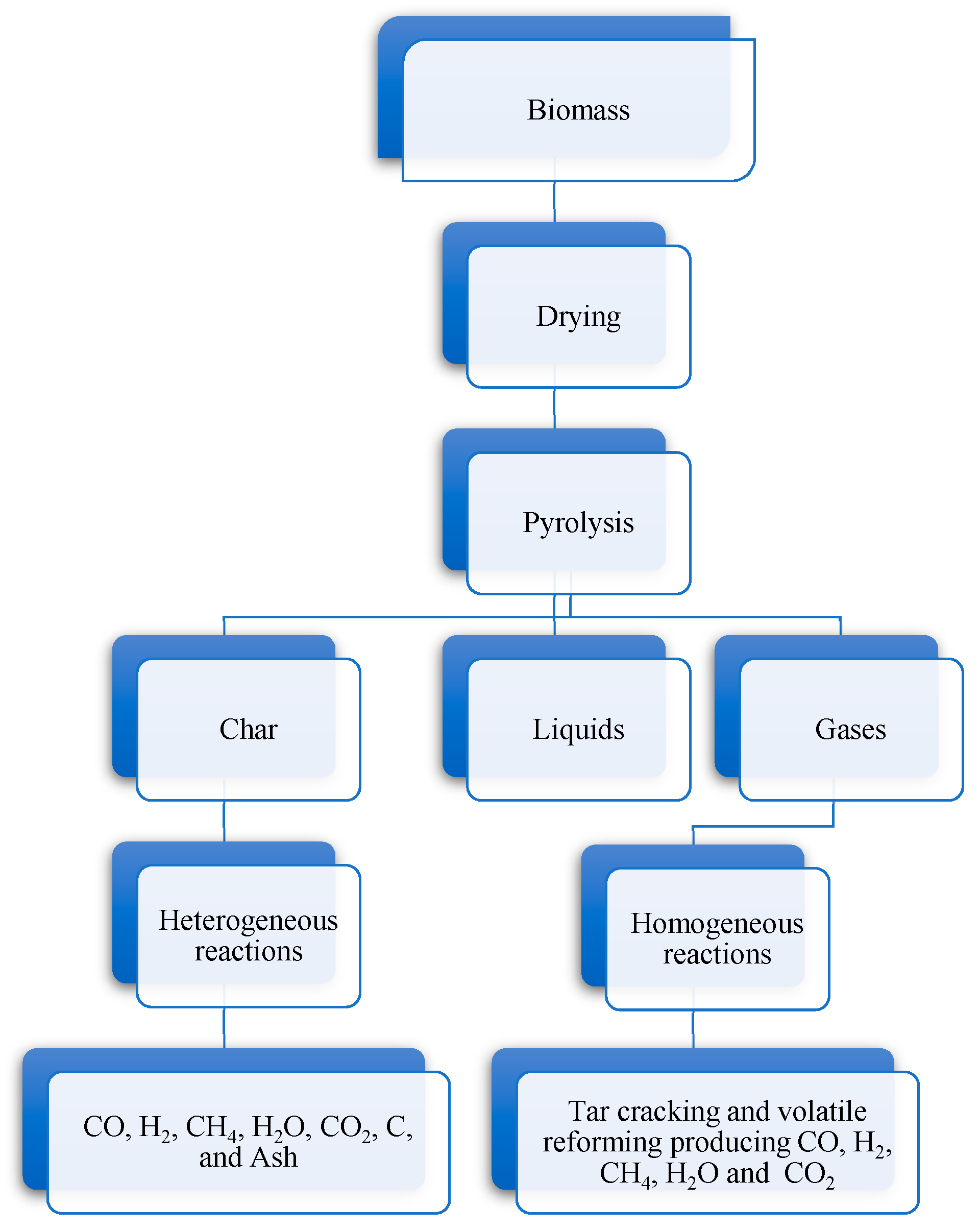
Figure 2.
General flowchart of a stoichiometric model.

Figure 3.
General flowchart of a non-stoichiometric model.


Table 1.
Summary of existing reviews on biomass gasification models.
| Authors | Review | Objectives |
|---|---|---|
| Gómez-Barea and Leckner (2010) [11] | Modeling of biomass gasification in fluidized bed | The objective of this article is to review the modeling of fluidized bed gasification of biomass and wastes. The work emphasizes the prediction of the performance of a fluidized bed biomass gasification in terms of gas composition, carbon conversion and gasification efficiency. |
| Puig-Arnavat et al. (2010) [12] | Review and analysis of biomass gasification models | The objective of this article is to review gasification process modelling in order to underline the role of gasification models. This review purposes to compare and analyze various biomass gasification models available in the literature. |
| Baruah and Baruah (2014) [13] | Modeling of biomass gasification: A review | The objective of this article is to review and compare some biomass gasification models available in the literature. A comparative study of the developed models is performed with emphasis on their applicability and limitations. |
| Loha et al. (2014) [22] | Advances in mathematical modeling of fluidized bed gasification | The objective of this article is to review the fluidized bed gasification models. Advantages and disadvantages of the modeling approaches and major results obtained are discussed. |
| Patra and Sheth (2015) [14] | Biomass gasification models for downdraft gasifier: A state-of-the-art review | The objective of this article is to review the current state-of-the- art of modeling of biomass gasification in fixed beds. A review of the gasification process is offered as departing point for the description of the gasification models. |
| Villetta et al. (2017) [29] | Modelling approaches to biomass gasification: A review with emphasis on the stoichiometric method | The objective of this article is to present a general overview of gasification models, highlighting those based on the stoichiometric method. The aim is to discuss the effect of biomass moisture content, equivalence ratio, pressure variations and oxygen enrichment on the quality of the produced gas. |
Table 2.
Thermodynamic modeling structures applied in biomass gasification. Adapted from [30].
Table 2.
Thermodynamic modeling structures applied in biomass gasification. Adapted from [30].
| Model Designation | Features |
|---|---|
| Thermodynamic equilibrium |
|
| Modified equilibrium models |
|
| Quasi-temperature model |
|
| Constrained free energy method |
|
Table 3.
Stoichiometric equilibrium models.
| Author(s) (Year) | Model’s Designation | Model Features |
|---|---|---|
| Zainal et al. (2001) [46] | Equilibrium model based on equilibrium constants | Global gasification reaction: Equilibrium is calculated by two independent reactions (3) and (9), three partial mass balances for C, H and O and one heat balance. The gasification temperature is fixed. Oxygen content and the produced gas composition are the unknowns. |
| Mountouris et al. (2006) [52] | Equilibrium model based on equilibrium constants | Global gasification reaction: Equilibrium is calculated using three independent reactions (2), (9) and (14), three partial mass balances (C, H and O) and by a heat balance. This model allows soot formation, as a solid carbon by-product (C) and exergy calculations for the process optimization. |
| Prins et al. (2007) [53] | Quasi-equilibrium model | Global biomass formula: CH1.4O0.6 Equilibrium is calculated by three independent reactions (1), (2), and (3), mass balances and heat balance. The model special feature is the use of the carbon boundary temperature (the temperature achieved when the exact quantity of oxygen is supplied and complete gasification is achieved). The quasi-equilibrium temperature approach was first introduced by Gumz [54], through which the equilibria of the reactions defined in the model are evaluated at a temperature lower than the process temperature. It can be concluded that the gasification efficiency is remarkable affected when the gasification reactions (9) and (10) are kinetically limited and do not contribute enough to the carbon conversion. The equilibrium model thus indicates the maximum efficiency that can be achieved. |
| Jarungthammachote and Dutta (2007) [42] | Thermodynamic equilibrium model based on equilibrium constants | Global gasification reaction: Equilibrium is calculated using two independent reactions (3) and (9), three partial mass balances (C, H and O) and a heat balance. The modification done to improve the model’s performance is the multiplication of equilibrium constants by coefficients. 11.28 and 0.91 are the coefficients used for the methanation and water-gas shift reactions, respectively. |
| Melgar et al. (2007) [55] | Thermochemical equilibrium model | Global gasification reaction: Two independent reactions (3) and (9), five partial mass balances (C, H, O, N, and S) and a heat balance calculate equilibrium. The equilibrium constants are calculated from the Gibbs free energy. This model introduces the sulfur in the biomass global formula and the corresponding formation of SO2 on the products side. |
| Sharma (2008) [56] | Equilibrium model of global reduction reactions | Global gasification reaction: Equilibrium is calculated by five partial mass balances (C, H, O, N and S), five reduction reactions (1), (2), (3), (9) and (14), and two approximations:
The equilibrium constants are calculated from the Gibbs free energy. |
| Huang and Ramaswamy (2009) [58] | Thermodynamic equilibrium model and modified model based on experimental compositions | Global gasification reaction: Equilibrium is calculated by three partial mass balances (C, H and O), and three independent reactions (2), (9) and (14). The equilibrium model is modified by adjusting the equilibrium constants of the reactions (9) and (14) based on experimental data. The coefficient factors were determined by fixing the fraction of CO and CH4 in the syngas from average experimental data values. |
| Abuadala et al. (2010) [59] | None | Global gasification reaction: Equilibrium is calculated by four partial mass balances (C, H, O and N), the independent reactions (3), and the following approximations for char and tar: |
| Karamarkovic and Karamarkovic (2010) [62] | Stoichiometric chemical equilibrium model and modified equilibrium models | The carbon boundary point (CBP) divided the model into two parts:
Equilibrium is calculated by four partial mass balances (C, H, O and N), by three independent reactions (1), (2), and (3) for the first part of the model and the reactions (9) and (11) for the second part of the model. Unknowns of the first part of the model are: temperature, amount of gasifying agent, amount and composition of produced gas. Unconverted carbon is defined only for the first part of the model. Unconverted carbon quantity is equal to zero, when gasification occurs at the CBP. Heterogeneous thermodynamic equilibrium of the produced gas and a given amount of unconverted carbon are calculated in the first part of the model. To achieve a better agreement with the experimental data, the reactions (9) and (11) are multiplied by 0.63 and 420, respectively. The artificial temperature differences for these reactions are 164 K and –226 K (referred by Prins et al. [53] as quasi-equilibrium temperatures). |
| Ngo et al. (2011) [63] | Quasi-equilibrium three-stage model | The three main stages in which this model is divided are:
Stage 1: pyrolysis Equilibrium is calculated by three mass balances (C, H, and O) and the following empirical equations derived on the basis of experimental data: Stage 2: char–gas reactions Equilibrium is calculated by three independent reactions (1), (2), and a secondary char-steam reaction C + 2H2O = CO2 + 2H2 The ratio of steam involved in the char–gas equilibrium reactions (β) is estimated from experimental data: Stage 3: gas-phase reactions Only the water–gas shift reaction is considered (Equation ((9)) being the equilibrium constant corrected by a non-equilibrium factor (κ) |
| Puig-Arnavat et al. (2012) [64] | Modified thermodynamic equilibrium model based on equilibrium constants | Biomass chemical formula was defined as CHxOyNz. All products leaving the gasifier were considered in the gas phase (H2, CO, CH4, CO2, H2O and N2). Preheated air and steam were used as gasifying agents. A pure thermodynamic equilibrium model was used following the procedure described by Zainal et al. [46] or Jarungthammachote and Dutta [42] along with the following modifications:
|
| Azzone et al. (2012) [65] | Equilibrium model | Global gasification reaction: Equilibrium is calculated by three partial mass balances (C, H, and O) by two independent reactions ((3) and (9)) and a heat balance. To consider that not all the carbon participates in the equilibrium reactions, a carbon fraction participating factor (α) was introduced representing the carbon that participates in the equilibrium reactions, while the remaining carbon by-passes the reaction zone. The molar amount of carbon that by-passes the chemical equilibrium is equal to (1 – α) = (1 − δ), being the parameter δ a function of ER defined as follows: |
| Barman et al. (2012) [66] | Realistic equilibrium model | Global gasification reaction: Equilibrium is calculated by three partial mass balances (C, H, and O), by three independent reactions (3), (9) and (11) and a heat balance. Tar is modeled with the chemical formula CH1.003O0.33 and its yield is assumed to be 4.5% (mass percentage). The Equilibrium model is modified by adjusting the equilibrium constant of the methane reaction that is multiplied by 3.5. |
| Silva and Rouboa (2013) [67] | Two-stage equilibrium model | Global gasification reaction: Equilibrium is calculated by three partial mass balances (C, H, and O), by five independent reactions (1)–(3), (9) and (11) and a heat balance. The equilibrium model is called two-stage due to the division in two stages:
This model is considered a modified equilibrium model because the methodology proposed by Jarungthammachote and Dutta [42] to correct the equilibrium constants by means of multiplicative factors was applied. |
| Lim and Lee (2014) [34] | Quasi-equilibrium thermodynamic model with empirical equations | Global gasification reaction: is the heat of the reaction at the standard temperature and pressure, i.e., 25 °C and 1 bar. Equilibrium is calculated by three partial mass balances (C, H, and O), by two independent reactions (3) and (9) and a heat balance. The unconverted carbon is obtained by a correlation 1 − fc based on experimental data of steam fluidized bed gasification. The carbon conversion factor fc used was: The model is modified by including multiplicative factors to correct the equilibrium constants of the reactions (3) and (9) obtained based on 43 experimental data sets for fluidized bed gasifiers as a function of the equivalence ratio: |
| Mendiburu et al. (2014) [68] | Equilibrium models and quasi-equilibrium model | Global gasification reaction: Equilibrium is calculated by three partial mass balances (C, H, and O), by five independent reactions (1)–(3), (9) and (11) and a heat balance. In the present work unconverted carbon is not considered. The pure equilibrium model is modified given rise to three models:
|
| Costa et al. (2015) [70] | Thermo-chemical equilibrium model | Global gasification reaction: Tar is modeled as benzene (C6H6) and its yield is supposed to obey the following empirical relation: Tar = 35.98 exp(−0.0029T) as in Abuadala et al. [59]. Equilibrium is calculated by three partial mass balances (C, H, and O), by three independent reactions (1), (3) and (9) and a heat balance. The equilibrium model is modified by multiplying the equilibrium constant of the three independent reactions (1), (3) and (9) by 0.58, 11.9 and 0.02, respectively. An optimization objective function is used to minimize the error between the numerical results of the syngas composition and the experimental measurements. |
| Rupesh et al. (2015) [71] | Stoichiometric quasi-steady-state model | Global gasification reaction: Tar is modeled as benzene (C6H6) and its yield is supposed to obey the following empirical relation: Tar = 35.98 exp(−0.00298T) as in Abuadala et al. [59] α is a carbon conversion factor expressed as a function of equivalence ratio (ER) and temperature (T): as in Lim and Lee [34]. Equilibrium is calculated by four partial mass balances (C, H, O and N) and by two independent reactions (3) and (9). The equilibrium model is modified by multiplying the equilibrium constant of the independent reactions (3) and (9) by coefficients as function of ER, 0.12e3.2ER and 41–50ER, respectively. These correction coefficients are obtained by minimizing the RMS error between the numerical results of the syngas composition and the experimental measurements. |
| Gagliano et al. (2016) [72] | Robust numerical model | Global gasification reaction: Equilibrium is calculated by three partial mass balances (C, H, and O), by two independent reactions (3) and (9) and a heat balance. Tar is modeled as C6H6.2O0.2 as in Adams [73] and the thermochemical properties assumed to be the same as benzene. The tar and char yields are fixed at 4.5% and 10.5% (mass percentage), respectively. |
| Aydin et al. (2017) [74] | semi-empirical equilibrium model | Global gasification reaction: Tar is assumed to be benzene (C6H6) and ϕ is the carbon fraction factor equal to: Equilibrium is calculated by three partial mass balances (C, H, and O), by two independent reactions (3) and (9), one heat balance and an equivalence correlation function of biomass oxygen content given by: The equilibrium constants of the water-gas shift and methanation reactions are multiplied by coefficients obtained by fitting the model with experimental data within the temperature range of 973–1390 K and the ER range of 0.21–0.5 in order to increase the accuracy of the results: |
Table 4.
Non-stoichiometric equilibrium models.
| Author(s) (Year) | Model Designation | Model Features | |
|---|---|---|---|
| Altafini et al. (2003) [18] | Equilibrium model based on minimization of the Gibbs free energy | The model contains equations of the:
The Gibbs free energy minimization is reached by the Lagrange multipliers method and the non-linear equation system is solved by the Newton–Raphson method. | |
| Li et al. (2004) [90] | Non-stoichiometric equilibrium model based on direct minimization of Gibbs free energy | Equilibrium is calculated by the minimization of Gibbs free energy using the Lagrange multipliers, mass balances, and energy conservation equation. 42 gaseous and two solid species involving C, H, O, N and S are considered. The model is modified to consider non-equilibrium effects of pyrolysis products like carbon and methane. An availability function is applied to each element, leading to a modified element amount vector affecting the gas, and assuming complete conversion for all elements other than carbon and hydrogen: b = (βcnc, βHnH, nO, nN, nS). The fraction of carbon converted into gaseous species is: βC,1 = 0.25 + 0.75e(-ER/0.23). A fraction of the carbon leaves the system without achieving equilibrium and is produced during the pyrolysis stage. That fraction entering the gas phase exists as methane. Experimental mass balance calculations suggest that this fraction can be approximated by: βc,2 = 0.11(1 − ER). The availability of carbon (overall fraction of carbon entering chemical equilibrium) is: β = βc,1 − βc,2. The availability of hydrogen at equilibrium (one mole of methane comprehends four moles of hydrogen atoms) is: βH = 1 − (4βC,2nC/nH). It is assumed that the reaction system is controlled by non-equilibrium factors and is composed by a mainstream in chemical equilibrium and a bypass zone. | |
| Jarungthammachote and Dutta (2008) [91] | Equilibrium modeling of gasification: Gibbs free energy minimization approach | The model considers that the produced gas is composed by six main components (H2, CO, CO2, CH4, N2 and H2O). Equilibrium is calculated by the minimization of the Gibbs free energy using the Lagrange multipliers and an energy balance assuming a heat loss of 1% of the HHV of the feedstock as in Altafini et al. [18]. The model is modified introducing the carbon conversion effect in the model:
| |
| Baratieri et al. (2010) [85] | Thermodynamic equilibrium model | Equilibrium is calculated by the minimization of the Gibbs free energy using the Lagrange multipliers and an energy balance. The non-linear system is solved using the Newton–Raphson method as in Altafini et al. [18]. The equilibrium model was modified to consider the residual char formed and the methane concentration. To calibrate the model, the measured concentration of hydrocarbons (CH4 and C2H4) and the amount of char collected were considered through:
| |
| Barba et al. (2011) [88] | Gibbs free energy gradient method model | Global gasification reaction Equilibrium is calculated by the minimization of Gibbs free energy, four mass balances (C, H, O and N), two equilibrium reactions (9) and (14), and an energy balance. Two steps were used to model the gasification process. In the first step, RDF is decomposed to produce a carbonaceous residue and a primary gas represented by: In the second step, the produced gas composition of the first step is modified by the water shift (9) and steam reforming (14) reactions. In this model an unreacted solid carbonaceous residue is formed and considered insensitive to process operating conditions. Consequently, two parameters (δ and γ) are defined as function of gasifying medium/feedstock ratio and reaction temperature: Steam: Air: Where ; | |
| Buragohain et al. (2012) [83] | Semi-equilibrium non-stoichiometric thermodynamic model | Equilibrium is calculated minimizing the Gibbs free energy using the Lagrange multipliers method and subjecting mass balance to constraints and an energy balance. To modify the model, the extent of carbon conversion was considered. The designation semi-equilibrium comes from the carbon conversion being taken as an independent parameter; four levels of carbon conversion (70, 80, 90, 100%) were considered. FACTSAGE software was used to carried out simulations. | |
| Materazzi et al. (2013) [49] | Thermodynamic equilibrium model | This equilibrium model follows the overall framework of single-stage equilibrium models. The system considers 43 different species. The ashes are inert but considered as part of thermal capacity in the reactor. Heat losses (Qloss) in the respective gasification phase is estimated to be 10% of the HHV of the feedstock supplied in the conversion phase. The thermodynamic equilibrium model of a two-stage process is formulated as follows: The char (solid carbon) is further converted in a steam–oxygen environment according to: The model uses the correlations given by Matsui et al. [92] and Linjewile et al. [94] with splitting factors 1.3 and 1.2 for the temperature range of 700–800 °C. A solid carbonaceous residue constitutes the unreacted solid from the first stage. The equilibrium is calculated, including the preliminary conversion process, by the minimization of the objective function, mass and energy balances for the two sequential stages. The solver applies the generalized reduced gradient method to solve the nonlinear system. | |
| Sreejith et al. (2013) [93] | Gibbs free energy minimization model | Equilibrium for steam gasification is calculated minimizing the Gibbs free energy. The gases are treated as real gases using the Redlich–Kwong equation of state. The mixture properties are computed based on the Amagat’s law. Minimization is performed in each iterative loop till the convergence of the mixture compressibility factor is achieved using the simulating annealing algorithm. This model is proposed in order to arrive at the optimum values for the reactor working parameters of temperature and pressure. Global gasification reaction: CxHyOz + aH2O + heat → bCO + dCO2 + eH2 + fCH4 + gH2O The constraints are elemental balances of C, H, and O as obtained from the global gasification chemical reaction and the non-negativity constraint | |
| Kangas et al. (2014) [30] | Super-equilibrium with the constrained Gibbs energy method | A chemical system with 14 species in the gaseous phase (H2, CO, CH4, C2H2, C2H4, C2H6, C3H8, C6H6, C10H8, NH3, O2, N2, H2O, SO2), water in liquid phase (H2O) and char and ash (C and SiO2) in the solid phases is considered. Equilibrium is calculated by the minimization of the Gibbs free energy via the Lagrange multipliers. The following constraints were considered: | |
| Constraint | Expression (mol/kg dry biomass) | ||
| C in char | 71.664 + 0.012906 × (T/K) | ||
| C in tar | 3.0 | ||
| N in ammonia | 0.042 | ||
| C in hydrocarbons | 17.642 − 0.009545 × (T/K) | ||
| H in hydrocarbons | 50.376 − 0.02732 × (T/K) | ||
| C in unsaturated and aromatic hydrocarbons | 3.9261 − 0.00208 × (T/K) | ||
| CH4 | 7.074 − 0.003 × (T/K) | ||
| C2H2 | 0.06454 − 0.00004 × (T/K) | ||
| C2H4 | 2.987 − 0.002 × (T/K) | ||
| C2H6 | 1.196 − 0.001 × (T/K) | ||
| C3H8 | 0.150921 − 0.000155 × (T/K) | ||
| C6H6 | 0.27 | ||
Six methods for modeling of global or local equilibrium were implemented:
| |||
| Mendiburu et al. (2014) [86] | Thermochemical equilibrium modeling: Constrained and unconstrained non-stoichiometric models | Global gasification reaction Equilibrium is calculated by the minimization of Gibbs free energy using the Lagrange multipliers, three mass balances (C, H and O) and a heat balance. Four models were developed: M1—Pure non-stoichiometric equilibrium model M2—non-stoichiometric constrained equilibrium model - methane content was constrained by the following empirical correlation: where the variables X1, X2 and X3 are the hydrogen to moisture content in the biomass, the normalized equivalence ratio and normalized gasification temperature, respectively. M3—kinetic constraint that determines the apparent gasification rate was considered. M4—implements simultaneously the two aforementioned constraints. | |
| Ghassemi and Markadeh (2014) [84] | Modified equilibrium model based on Gibbs free energy minimization | Global gasification reaction: Equilibrium is calculated by the minimization of Gibbs free energy using the Lagrange multipliers, three elemental mass balances (C, H and O) and a heat balance. The equilibrium model is modified by introducing carbon conversion and tar formation constraints. The carbon conversion expression of Azzone et al. [65] is implemented: Tar is modeled with the chemical formula CH1.003O0.33 and its yield is assumed to be 4.5% (mass percentage) as in Barman et al. [66] | |
| Yakaboylu et al. (2015) [89] | Constrained equilibrium model | The model comprises two parts:
The constraints included are the carbon and hydrogen gasification efficiencies and constrained amounts for specific compounds. A distinctive aspect of the model is the consideration of real gases using the Peng−Robinson equation of state. | |
| Vakalis et al. (2016) [32] | Multi-stage thermodynamic model: Multi-box approach | The multi-box approach is used due to the separation of the reactor into various processes, instead of using a conventional single-stage (also known as black-box) model approach.
| |
| Biagini et al. (2016) [33] | Bi-equilibrium model | The naming bi-equilibrium model finds explanation in the bypass of the oxidation zone of some pyrolysis products usually underestimated in equilibrium models. The model is developed considering the multi-phase nature of the gasification process:
The reactor heat losses were assumed to be 5% of the biomass thermal energy. The ash properties were assumed from SiO2. | |
| Gambarotta et al. (2018) [87] | Non-stoichiometric equilibrium model | Global gasification reaction: Equilibrium is calculated minimizing the Gibbs free energy, five mass balances (C, H, O, N and S) and an energy balance. α is the factor that takes into account the carbon not participating in the gasification. This factor is a function of the air-to-fuel ratio proposed by Azzone et al. [65] and firstly introduced by Li et al. [79]. Tar production is neglected. | |
© 2019 by the authors. Licensee MDPI, Basel, Switzerland. This article is an open access article distributed under the terms and conditions of the Creative Commons Attribution (CC BY) license (http://creativecommons.org/licenses/by/4.0/).
Share and Cite
MDPI and ACS Style
Ferreira, S.; Monteiro, E.; Brito, P.; Vilarinho, C. A Holistic Review on Biomass Gasification Modified Equilibrium Models. Energies 2019, 12, 160. https://doi.org/10.3390/en12010160
AMA Style
Ferreira S, Monteiro E, Brito P, Vilarinho C. A Holistic Review on Biomass Gasification Modified Equilibrium Models. Energies. 2019; 12(1):160. https://doi.org/10.3390/en12010160
Chicago/Turabian StyleFerreira, Sérgio, Eliseu Monteiro, Paulo Brito, and Cândida Vilarinho. 2019. "A Holistic Review on Biomass Gasification Modified Equilibrium Models" Energies 12, no. 1: 160. https://doi.org/10.3390/en12010160
Note that from the first issue of 2016, this journal uses article numbers instead of page numbers. See further details here.