Minimization of Losses in Solar Photovoltaic Modules by Reconfiguration under Various Patterns of Partial Shading


Abstract
:1. Introduction
2. Materials and Methods
2.1. Solar PV Module Equivalent Circuit and the Effect of Solar Radiation and Temperature
- Iph is the current generated from sunlight (A).
- I is the solar PV module’s current (A);
- Io is the reverse saturation current of the diode (A);
- V is the PV module’s voltage (V);
- Rs is the series resistance of the solar PV module (Ω);
- Rp is the parallel resistance of the solar PV module (Ω);
- q is the electron charge, which is 1.602 × 10⁻¹⁹ Coulombs;
- K is the Boltzmann constant, which is 1.3806504 × 10⁻²³ J/K;
- T is the operating temperature of the solar PV module (Kelvin);
- n is the ideality factor of the diode; and
- Ns is the number of cells per module.
- Iph,ref is the photo current at the temperature Tref (A);
- Iph,shade is the photo current at the temperature T (A);
- Vref is the open circuit voltage at the temperature of 25 °C (V);
- Voc,new is the open circuit voltage at operating temperature (V);
- KI is the temperature coefficients of the current (A/°C);
- KV is the temperature coefficients of the voltage; V/°C;
- Tref is the reference temperature of the solar PV module (Kelvin);
- Gref is the reference solar radiation (1000 W/m2); and
- Gshaded is the shaded solar radiation (W/m2).
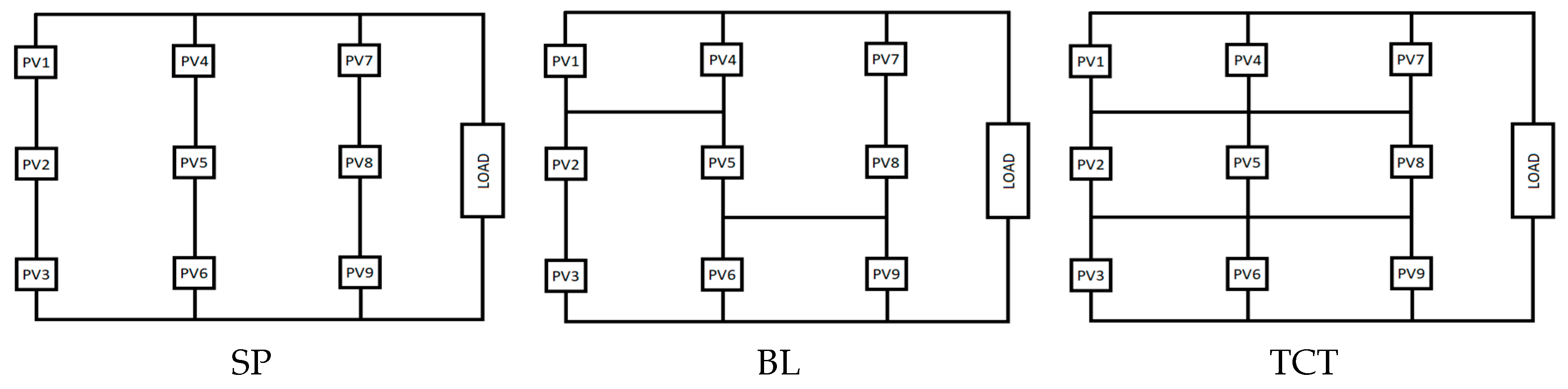
2.2. PV Module Configurations
2.3. Shading Patterns
2.4. Model of the 3 × 3 PV Modules
2.5. Minimum Loss Configuration
3. Results and Discussion
3.1. Comparative Results between the Ideal Switch and the Non-Ideal Switch
3.2. Minimum Loss Configuration (ML)
4. Conclusions
Author Contributions
Funding
Acknowledgments
Conflicts of Interest
References
- Department of Alternative Energy Development and Efficiency. Solar Radiation. 2015. Available online: http://www.dede.go.th (accessed on 26 July 2017).
- Department of Alternative Energy Development and Efficiency. Technology of Solar Cell. 2015. Available online: http://www.dede.go.th. (accessed on 26 July 2017).
- Electricity Generating Authority of Thailand. Solar Cell. 2015. Available online: www3.egat.co.th/re/solarcell/solarcell_pg5.htm (accessed on 26 July 2017).
- Durgadevi, A.; Arulselvi, S.; Natarajan, S.P. Photovoltaic Modeling and Its Characteristics. In Proceedings of the 2011 International Conference on Emerging Trends in Electrical and Computer Technology, ICETECT 2011, Nagercoil, India, 23–24 March 2011; pp. 469–475. [Google Scholar] [CrossRef]
- Ramos-Paja, C.A.; Bastidas, J.D.; Saavedra-Montes, A.J.; Guinjoan-Gispert, F.; Goez, M. Mathematical Model of Total Cross-Tied Photovoltaic Arrays in Mismatching Conditions. In Proceedings of the 2012 IEEE 4th Colombian Workshop on Circuits and Systems (CWCAS), Barranquilla, Colombia, 1–2 November 2012. [Google Scholar] [CrossRef]
- Storey, J.P.; Wilson, P.R.; Bagnall, D. Improved Optimization Strategy for Irradiance Equalization in Dynamic Photovoltaic Arrays. IEEE Trans. Power Electron. 2013, 28, 2946–2956. [Google Scholar] [CrossRef] [Green Version]
- Tabanjat, A.; Becherif, M.; Hissel, D. Reconfiguration Solution for Shaded PV Panels Using Switching Control. Renew. Energy 2015, 82, 4–13. [Google Scholar] [CrossRef]
- Pendem, S.R.; Mikkili, S. Modeling, Simulation and Performance Analysis of Solar PV Array Configurations (Series, Series–Parallel and Honey-Comb) to Extract Maximum Power under Partial Shading Conditions. Energy Rep. 2018, 4, 274–287. [Google Scholar] [CrossRef]
- Kumar, A.; Pachauri, R.K.; Chauhan, Y.K. Experimental Analysis of SP/TCT PV Array Configurations under Partial Shading Conditions. In Proceedings of the 2016 IEEE 1st International Conference on Power Electronics, Intelligent Control and Energy Systems (ICPEICES), Delhi, India, 4–6 July 2016; pp. 1–5. [Google Scholar] [CrossRef]
- Das, P.; Mohapatra, A.; Nayak, B. Modeling and Characteristic Study of Solar Photovoltaic System under Partial Shading Condition. Mater. Today Proc. 2017, 4, 12586–12591. [Google Scholar] [CrossRef]
- Jaideaw, W.; Suksri, A.; Wongwuttanasatian, T. Simulation of Photovoltaic Module Configuration for Different Shaded Patterns. IOP Conf. Ser. Earth Environ. Sci. 2018, 113, 012204. [Google Scholar] [CrossRef]
- Pachauri, R.; Singh, R.; Gehlot, A.; Samakaria, R.; Choudhury, S. Experimental Analysis to Extract Maximum Power from PV Array Reconfiguration under Partial Shading Conditions. Eng. Sci. Technol. Int. J. 2018, in press. [Google Scholar] [CrossRef]
- Srinivasa Rao, P.; Saravana Ilango, G.; Nagamani, C. Maximum Power from PV Arrays Using a Fixed Configuration under Different Shading Conditions. IEEE J. Photovolt. 2014, 4, 679–686. [Google Scholar] [CrossRef]
- Ramaprabha, R.; Mathur, B.L. MATLAB Based Modelling to Study the Influence of Shading on Series Connected SPVA. In Proceedings of the 2009 2nd International Conference on Emerging Trends in Engineering and Technology, ICETET 2009, Nagpur, India, 16–18 December 2009; pp. 30–34. [Google Scholar]
- Buddha, S.T. Topology Reconfiguration To Improve The Photovoltaic (PV) Array Performance. Master’s Thesis, Arizona State University, Tempe, AZ, USA, 2011. [Google Scholar]
- Jazayeri, M.; Uysal, S.; Jazayeri, K. A Comparative Study on Different Photovoltaic Array Topologies under Partial Shading Conditions. In Proceedings of the 2014 IEEE PES T&D Conference and Exposition, Chicago, IL, USA, 4-17 April 2014; pp. 1–5. [Google Scholar] [CrossRef]
- Bauwens, P.; Doutreloigne, J. Reducing Partial Shading Power Loss with an Integrated Smart Bypass. Sol. Energy 2014, 103, 134–142. [Google Scholar] [CrossRef]
- Deshkar, S.N.; Dhale, S.B.; Mukherjee, J.S.; Babu, T.S.; Rajasekar, N. Solar PV Array Reconfiguration under Partial Shading Conditions for Maximum Power Extraction Using Genetic Algorithm. Renew. Sustain. Energy Rev. 2015, 43, 102–110. [Google Scholar] [CrossRef]
- Dhanalakshmi, B.; Rajasekar, N. Dominance Square Based Array Reconfiguration Scheme for Power Loss Reduction in Solar PhotoVoltaic (PV) Systems. Energy Convers. Manag. 2018, 156, 84–102. [Google Scholar] [CrossRef]
- Pillai, D.S.; Prasanth Ram, J.; Siva Sai Nihanth, M.; Rajasekar, N. A Simple, Sensorless and Fixed Reconfiguration Scheme for Maximum Power Enhancement in PV Systems. Energy Convers. Manag. 2018, 172, 402–417. [Google Scholar] [CrossRef]
- Dhanalakshmi, B.; Rajasekar, N. A Novel Competence Square Based PV Array Reconfiguration Technique for Solar PV Maximum Power Extraction. Energy Convers. Manag. 2018, 174, 897–912. [Google Scholar] [CrossRef]
- Akrami, M.; Pourhossein, K. A Novel Reconfiguration Procedure to Extract Maximum Power from Partially-Shaded Photovoltaic Arrays. Sol. Energy 2018, 173, 110–119. [Google Scholar] [CrossRef]
- Satpathy, P.R.; Sharma, R. Power Loss Reduction in Partially Shaded PV Arrays by a Static SDP Technique. Energy 2018, 156, 569–585. [Google Scholar] [CrossRef]
- Bellia, H.; Youcef, R.; Fatima, M. A Detailed Modeling of Photovoltaic Module Using MATLAB. NRIAG J. Astron. Geophys. 2014, 3, 53–61. [Google Scholar] [CrossRef]
- Lekkruasuwan, A.; Chaitusaney, S.; Eua-arporn, B. Adaptive Photovoltaic Array Configuration for Alleviating Impact of Shading on Power Generation. In Proceedings of the 2014 11th International Conference on Electrical Engineering/Electronics, Computer, Telecommunications and Information Technology (ECTI-CON), Nakhon Ratchasima, Thailand, 14–17 May 2014; pp. 1–6. [Google Scholar] [CrossRef]
- Circuit Basics. 2018. Available online: www.circuitbasics.com/wp-content/uploads/2015/11/SRD-05VDC-SL-C-Datasheet.pdf (accessed on 5 October 2018).
- All about Circuits. Time-Delay Relays. 2018. Available online: www.allaboutcircuits.com/textbook/digital/chpt-5/time-delay-relays/ (accessed on 5 October 2018).
- Tubniyom, C.; Jaideaw, W.; Chatthaworn, R.; Suksri, A.; Wongwuttanasatian, T. Effect of Partial Shading Patterns and Degrees of Shading on Total Cross-Tied (TCT) Photovoltaic Array Configuration. Energy Procedia 2018, 153, 35–41. [Google Scholar] [CrossRef]


| Characteristics | Spec. |
|---|---|
| Maximum power (Pmax) | 20 W |
| Maximum power voltage (Vmax) | 17.6 V |
| Maximum power current (Imax) | 1.14 A |
| Open circuit voltage (Voc) | 21.4 V |
| Shot circuit current (Isc) | 1.57 A |
| Output tolerance (%) | ±3% |
| Characteristics | Spec. |
|---|---|
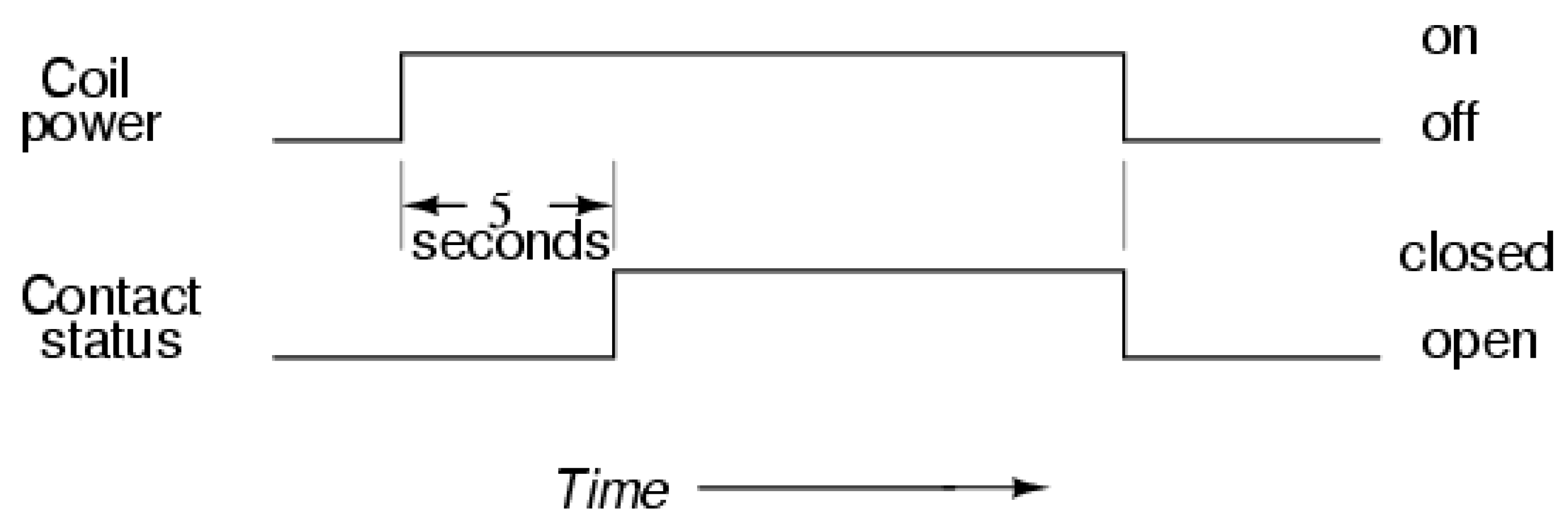
| Coil voltage (V) | 5 V |
| Nominal voltage (Vdc) | 5 V |
| Nominal current (I) | 71.4 mA |
| Coil resistance ±10% (Ω) | 70 Ω |
| Contact resistance (Ω) | 100 mΩ Max. |
| Power consumption (W) | abt. 0.36 W |
| Solar Radiation (W/m2) | and | |||||
|---|---|---|---|---|---|---|
| SP (W) | BL (W) | TCT (W) | ||||
| Ideal Switch | Non-Ideal Switch | Ideal Switch | Non-Ideal Switch | |||
| 1000 | 177.92 | 177.92 (0%) | 176.82 (−0.62%) | 177.92 (0%) | 175.72 (−1.24%) | |
| Light cloud | 900 | 174.92 | 175.4 (0.28%) | 174.26 (−0.38%) | 175.6 (0.39%) | 173.31 (−0.92%) |
| 800 | 169.09 | 171.2 (1.28%) | 170.08 (0.58%) | 171.8 (1.60%) | 169.63 (0.32%) | |
| 700 | 162.47 | 165.9 (2.11%) | 164.80 (1.43%) | 167.1 (2.86%) | 164.86 (1.47%) | |
| Medium dark cloud | 600 | 154.98 | 160.0 (3.24%) | 158.88 (2.52%) | 161.8 (4.40%) | 159.54 (2.94%) |
| 500 | 146.76 | 153.6 (4.66%) | 152.49 (3.91%) | 156.1 (6.37%) | 153.88 (4.85%) | |
| 400 | 137.94 | 146.8 (6.43%) | 145.73 (5.65%) | 150.2 (8.89%) | 147.93 (7.24%) | |
| Dark cloud | 300 | 128.61 | 139.8 (8.70%) | 138.64 (7.80%) | 144 (11.97%) | 141.71 (10.19%) |
| 200 | 118.82 | 132.4 (11.43%) | 131.25 (10.46%) | 137.5 (15.72%) | 135.24 (13.81%) | |
| 100 | 109.87 | 124.7 (13.50%) | 123.58 (12.48%) | 130.8 (19.05%) | 128.52 (16.98%) | |
| Solar Radiation (W/m²) | and | ||||||||
|---|---|---|---|---|---|---|---|---|---|
| Case 3 (22% Shaded) | Case 4 (22% Shaded) | Case 5 (44% Shaded) | Case 6 (44% Shaded) | ||||||
| BL | TCT | BL | TCT | BL | TCT | BL | TCT | ||
| 1000 | −0.62% | −1.24% | −0.62% | −1.24% | −0.62% | −1.24% | −0.62% | −1.24% | |
| Light cloud | 900 | −0.60% | −0.94% | −0.49% | −0.75% | −0.38% | −0.98% | 0.20% | 0.26% |
| 800 | −0.59% | −0.42% | −0.34% | 0.07% | −0.01% | −0.64% | 2.35% | 3.12% | |
| 700 | −0.57% | 0.04% | −0.09% | 1.39% | 0.47% | −0.21% | 5.76% | 7.31% | |
| Medium dark cloud | 600 | −0.56% | 0.53% | 0.35% | 3.31% | 1.13% | 0.38% | 11.24% | 14.08% |
| 500 | −0.56% | 1.11% | 1.00% | 5.97% | 2.00% | 1.15% | 11.02% | 15.56% | |
| 400 | −0.58% | 1.81% | 1.93% | 9.69% | 3.12% | 2.14% | −5.05% | 0.87% | |
| Dark cloud | 300 | −0.60% | 2.63% | −3.13% | −4.24% | 4.61% | 3.43% | −21.22% | −13.93% |
| 200 | −0.72% | 3.60% | −3.13% | −7.68% | 6.64% | 5.18% | −37.23% | −28.66% | |
| 100 | −0.87% | 4.72% | −3.13% | −7.72% | 9.54% | 7.63% | −52.77% | −43.11% | |
| Solar Radiation (W/m2) | % Difference in Total Power | ||||||||
| NONE (SP) | SW 1 | SW 2 | SW 3 | SW 4 | SW 1, 2 | SW 1, 3 (ML) | SW 1, 4 (BL) | ||
| 1000 | 0.00% | −0.31% | −0.31% | −0.31% | −0.31% | −0.62% | −0.62% | −0.62% | |
| Light cloud | 900 | 0.00% | −0.10% | −0.36% | −0.50% | −0.50% | −0.41% | −0.27% | −0.38% |
| 800 | 0.00% | 0.75% | 0.03% | −0.33% | −0.33% | 0.43% | 0.97% | 0.58% | |
| 700 | 0.00% | 1.51% | 0.21% | −0.34% | −0.34% | 1.17% | 2.14% | 1.43% | |
| Medium dark cloud | 600 | 0.00% | 2.51% | 0.43% | −0.35% | −0.35% | 2.15% | 3.65% | 2.52% |
| 500 | 0.00% | 3.77% | 0.73% | −0.37% | −0.37% | 3.39% | 5.60% | 3.91% | |
| 400 | 0.00% | 5.33% | 1.13% | −0.40% | −0.40% | 4.93% | 8.04% | 5.65% | |
| Dark cloud | 300 | 0.00% | 7.24% | 1.65% | −0.43% | −0.43% | 6.81% | 11.05% | 7.80% |
| 200 | 0.00% | 9.58% | 2.31% | −0.46% | −0.46% | 9.12% | 14.74% | 10.46% | |
| 100 | 0.00% | 11.21% | 1.98% | −0.50% | −0.50% | 10.71% | 17.98% | 12.48% | |
| Solar Radiation (W/m2) | % Difference in Total Power | ||||||||
| SW 2, 3 | SW 2, 4 | SW 3, 4 | SW 1, 2, 3 | SW 1, 2, 4 | SW 1, 3, 4 | SW 2, 3, 4 | SW 1, 2, 3, 4 (TCT) | ||
| 1000 | −0.62% | −0.62% | −0.62% | −0.93% | −0.93% | −0.93% | −0.93% | −1.24% | |
| Light cloud | 900 | −0.67% | −0.62% | −0.81% | −0.58% | −0.68% | −0.58% | −0.93% | −0.92% |
| 800 | −0.27% | −0.08% | −0.65% | 0.64% | 0.28% | 0.64% | −0.41% | 0.32% | |
| 700 | −0.08% | 0.25% | −0.68% | 1.81% | 1.12% | 1.81% | −0.09% | 1.47% | |
| Medium dark cloud | 600 | 0.16% | 0.64% | −0.71% | 3.30% | 2.18% | 3.30% | 0.29% | 2.94% |
| 500 | 0.49% | 1.17% | −0.75% | 5.23% | 3.56% | 5.23% | 0.80% | 4.85% | |
| 400 | 0.94% | 1.87% | −0.80% | 7.64% | 5.28% | 7.64% | 1.48% | 7.24% | |
| Dark cloud | 300 | 1.51% | 2.78% | −0.86% | 10.62% | 7.41% | 10.62% | 2.35% | 10.19% |
| 200 | 2.22% | 3.91% | −0.93% | 14.28% | 10.04% | 14.28% | 3.45% | 13.81% | |
| 100 | 1.96% | 4.16% | −1.00% | 17.48% | 12.04% | 17.48% | 3.66% | 16.98% | |
| Solar Radiation (W/m²) | and | |||||||||
|---|---|---|---|---|---|---|---|---|---|---|
| Case 2 (11% Shaded) | Case 3 (22% Shaded) | Case 4 (22% Shaded) | Case 5 (44% Shaded) | Case 6 (44% Shaded) | ||||||
| ML SW 1, 3 | TCT | ML SW 2, 4 | TCT | ML SW 3 | TCT | ML SW 4 | BL | ML (TCT) | ||
| 1000 | −0.62% | −1.24% | −0.62% | −1.24% | −0.31% | −1.24% | −0.31% | −1.24% | −1.24% | |
| Light cloud | 900 | −0.27% | −0.92% | −0.30% | −0.94% | 0.10% | −0.75% | −0.06% | −0.98% | 0.26% |
| 800 | 0.97% | 0.32% | 0.24% | −0.42% | 0.85% | 0.07% | 0.34% | −0.64% | 3.12% | |
| 700 | 2.14% | 1.47% | 0.73% | 0.04% | 2.07% | 1.39% | 0.87% | −0.21% | 7.31% | |
| Medium dark cloud | 600 | 3.65% | 2.94% | 1.22% | 0.53% | 3.92% | 3.31% | 1.59% | 0.38% | 14.08% |
| 500 | 5.60% | 4.85% | 1.88% | 1.11% | 6.52% | 5.97% | 2.52% | 1.15% | 15.56% | |
| 400 | 8.04% | 7.24% | 2.63% | 1.81% | 10.19% | 9.69% | 3.74% | 2.14% | 0.87% | |
| Dark cloud | 300 | 11.05% | 10.19% | 3.52% | 2.63% | 0.99% | −4.24% | 5.36% | 3.43% | −13.93% |
| 200 | 14.74% | 13.81% | 4.55% | 3.60% | −1.58% | −7.68% | 7.59% | 5.18% | −28.66% | |
| 100 | 17.98% | 16.98% | 5.74% | 4.72% | −4.41% | −7.72% | 10.82% | 7.63% | −43.11% | |
© 2018 by the authors. Licensee MDPI, Basel, Switzerland. This article is an open access article distributed under the terms and conditions of the Creative Commons Attribution (CC BY) license (http://creativecommons.org/licenses/by/4.0/).
Share and Cite
Tubniyom, C.; Chatthaworn, R.; Suksri, A.; Wongwuttanasatian, T. Minimization of Losses in Solar Photovoltaic Modules by Reconfiguration under Various Patterns of Partial Shading. Energies 2019, 12, 24. https://doi.org/10.3390/en12010024
Tubniyom C, Chatthaworn R, Suksri A, Wongwuttanasatian T. Minimization of Losses in Solar Photovoltaic Modules by Reconfiguration under Various Patterns of Partial Shading. Energies. 2019; 12(1):24. https://doi.org/10.3390/en12010024
Chicago/Turabian StyleTubniyom, Chayut, Rongrit Chatthaworn, Amnart Suksri, and Tanakorn Wongwuttanasatian. 2019. "Minimization of Losses in Solar Photovoltaic Modules by Reconfiguration under Various Patterns of Partial Shading" Energies 12, no. 1: 24. https://doi.org/10.3390/en12010024
APA StyleTubniyom, C., Chatthaworn, R., Suksri, A., & Wongwuttanasatian, T. (2019). Minimization of Losses in Solar Photovoltaic Modules by Reconfiguration under Various Patterns of Partial Shading. Energies, 12(1), 24. https://doi.org/10.3390/en12010024