A Simplified Model Predictive Control for T-Type Inverter with Output LC Filter

Abstract

In this paper, a model predictive control scheme for the T-type inverter with an output LC filter is presented. A simplified dynamics model is proposed to reduce the number of the measurement and control variables, resulting in a decrease in the cost and complexity of the system. Furthermore, the main contribution of the paper is the approach to evaluate the cost function. By employing the selection of sector information distribution in the reference inverter voltage and capacitor voltage balancing, the execution time of the proposed algorithm is significantly reduced by 36% compared with conventional model predictive control without too much impact on control performance. Simulation and experimental results are studied and compared with conventional finite control set model predictive control to validate the effectiveness of the proposed method.

1. Introduction

Recently, the multilevel converter has been widely applied to various applications such as renewable energy system, flexible AC transmission systems and electric drives thanks to its benefits: increase the power capacity of the converter and improve the quality of the system [1,2,3]. In particular, compared with the neutral-point-clamped (NPC) type, the T-type inverter topology has the advantage in terms of the efficiency for medium switching frequency [4,5,6]. Thus, the T-type inverter is considered to be an alternative solution for multilevel inverter. Like the NPC converter, the unbalance of neutral-point potential is the drawback of this topology which causes the distortion of the output voltage and current. However, several approaches have been introduced to solve this problem [7,8,9,10].

A linear controller with proportional-integral (PI) is typically applied to control the converter because of its simplicity and stability [11,12]. However, this approach has a low dynamic response and requires a complex modulation technique for balancing the DC-link capacitor voltage. Recently, direct power control [13] which uses a switching look-up table for determining the switching state has been introduced to improve the performance. Nonetheless, it requires a high sampling frequency to achieve an acceptable steady-state and high dynamic performances. To deal with this disadvantage, several control approaches have been proposed such as using direct power control with space vector modulation [14], fuzzy control [15], sliding mode control [16], and predictive control [17,18,19].

In recent years, a finite control set model predictive control (FCS-MPC) is considered as an attractive alternative control strategy for power converters due to its simple structure, facilitating implementation, and fast dynamic response [20,21,22,23,24,25]. Furthermore, compared with classical control, the FCS-MPC provides the advantages such as easy inclusion of nonlinearities and constraints in the controller. However, at each sampling period, the prediction of control variables is 27, corresponding to the three-level T-type inverter, leading to producing a high computational cost. In [26], a simplified FCS-MPC for three-level voltage source converter is introduced. In order to reduce the computational time, this approach used the two-level switching state group for prediction and optimization. Another approach is presented in [27], which employs equivalent transformations in the cost function for the optimization loop. Another approach is proposed in [28,29] based on using a modified sphere decoding algorithm for multilevel converters. In [30], a sector distribution and non-zero voltage vectors are exploited with the aim to reduce the computational burden for two-level converters. Nonetheless, the main disadvantage of this method is the nonexistence of zero voltage leading to an increase of the total harmonic distortion (THD) in the load current. In [31], the control approach is suggested based on the candidate region that minimizes the sub-cost function to reduce the execution time. The presented technique in [32] combined the conventional FCS-MPC, a look-up table, and steady-state evaluation to reduce the computational burden. However, this algorithm can have a large amount of computational cost like the conventional FCS-MPC in the worst case.

With a three-level T-type inverter, control variables are predicted by using the predictive model and measured variables such as DC-link capacitor voltage, output voltage, filter current, and output current. In order to reduce the cost and complexity of this system, a simplified dynamics model is presented in this paper. Moreover, the highlight of this research is the significant computational cost reduction without decreasing the quality of control by preselecting the required inverter output voltage. The balance of DC-link capacitor voltage is guaranteed by determining the suitable small voltage vectors resulting in the elimination of the weighting factor in the cost function. As a consequence, the amount of predictive state for loop optimization is reduced from 27 to 6 compared with the conventional FCS-MPC method. This means that it is easy to implement the proposed algorithm in a real-time system with a low-cost processor and to extend with a long prediction horizon for improving the control performance. The simulation and experimental results validate the effectiveness of the proposed control strategy.

The rest of this paper is organized as follows: a reduced model predictive control for the three-level T-type inverter is presented in Section 2. Next, the proposed algorithm is explained in Section 3 for reducing the computational cost. In Section 4, a comparative study of the conventional FCS-MPC and the proposed method is examined. Finally, the conclusions are given in Section 5.

2. Model Predictive Control for a Three-Level T-Type Inverter

2.1. Topology

A simple topology of the three-level T-type inverter (3L-T-type) is shown in Figure 1. The basic principle of this configuration can be expressed by three switching states [P], [N] and [O] which correspond to three inverter output voltages $+U_{dc}/2$, $-U_{dc}/2$ and 0. Consequently, 27 possible switching configurations are considered for a 3L-T-type inverter.

Table 1. Operating status of inverter leg x $\in \left\{a,b,c\right\}$.

State	Switch				Inverter Output Voltage
${\mathit{S}}_{\mathit{x}}$	${\mathit{S}}_{\mathbf{1}\mathit{x}}$	${\mathit{S}}_{\mathbf{2}\mathit{x}}$	${\mathit{S}}_{\mathbf{3}\mathit{x}}$	${\mathit{S}}_{\mathbf{4}\mathit{x}}$	${\mathit{u}}_{\mathit{xZ}}$
P	1	1	0	0	$U_{dc}/2$
O	0	1	1	0	0
N	0	0	1	1	$-U_{dc}/2$

presents the summary of the operating principle for 3L-T-type.

2.2. Mathematical Modeling of the System

The inverter output voltage produced by the 3L-T-type inverter is given by:

$$u_{inv}={\displaystyle \frac{2}{3}}\left(u_{AZ}+k{u}_{BZ}+k^2{u}_{CZ}\right),$$

(1)

where $u_{AZ}$, $u_{BZ}$, and $u_{CZ}$ are the output phase voltages; $k=e^{j2\pi /3}=-\frac{1}{2}+j\frac{\sqrt{3}}{2}$.

The phase voltage $u_{xZ}$ is calculated in terms of DC-link voltage $U_{dc}$ and switching state $S_x$ as [9,22]:

$$u_{xZ}=S_x\frac{U_{dc}}{2},$$

(2)

where $S_x$ represents the switching status and has three possible values: $\{-1,0,1\}$ with the index $x\in \left\{a,b,c\right\}$.

The dynamic behavior of LC filter can be described by the following:

$$\begin{array}{cc}\hfill L_f\frac{d{i}_f}{dt}& =u_{inv}-u_c,\hfill \\ \hfill C_f\frac{d{u}_c}{dt}& =i_f-i_o,\hfill \end{array}$$

(3)

where $u_{inv}$ and $u_c$ are the inverter and output capacitor voltage vectors; $i_f$ and $i_o$ are the filter and output load current vectors and $L_f$, $C_f$ are the filter inductance and capacitance.

The control variables $u_c$ and $i_f$ are measured while $u_{inv}$ is obtained from Equations (1) and (2). In general, $i_o$ is measured or estimated by using an observer, leading to an increase in the cost and complexity of the system. In this paper, to achieve a simple model, we assume that the output load current is derived from output capacitor voltage. Thus, Equation (3) is rewritten as:

$$\begin{array}{cc}\hfill \frac{d{u}_c}{dt}& =\frac{1}{C_f}\left(i_f-\frac{u_c}{R_{Load}}\right),\hfill \\ \hfill \frac{d{i}_f}{dt}& =\frac{1}{L_f}\left(u_{inv}-u_c\right),\hfill \end{array}$$

(4)

where $R_{load}$ is the load resistance.

In order to reduce the number of the control variable, the neutral-point voltage is taken into account in the model instead of two capacitor voltages ($u_{C1}$, $u_{C2}$). The neutral-point voltage ($u_z$) can be expressed based on the assumption that the DC-link voltage is kept constant and $C_1$ = $C_2$ = C as follows:

$$\begin{array}{c}{\displaystyle \frac{d{u}_z}{dt}}={\displaystyle \frac{d\left(u_{C1}-u_{C2}\right)}{dt}}=-{\displaystyle \frac{1}{C}}{i}_z=-{\displaystyle \frac{1}{C}}\left((1-|S_a|)i_{fa}+(1-|S_b|)i_{fb}+(1-|S_c|)i_{fc}\right).\hfill \end{array}$$

(5)

Consequently, we have a representation of the dynamics model based on Equations (4) and (5) as:

$$\begin{array}{c}\frac{d{u}_c}{dt}=\frac{1}{C_f}\left(i_f-\frac{u_c}{R_{Load}}\right),\hfill \\ \frac{d{i}_f}{dt}=\frac{1}{L_f}\left(u_{inv}-u_c\right),\hfill \\ {\displaystyle \frac{d{u}_z}{dt}}=-{\displaystyle \frac{1}{C}}\left((1-|S_a|)i_{fa}+(1-|S_b|)i_{fb}+(1-|S_c|)i_{fc}\right).\hfill \end{array}$$

(6)

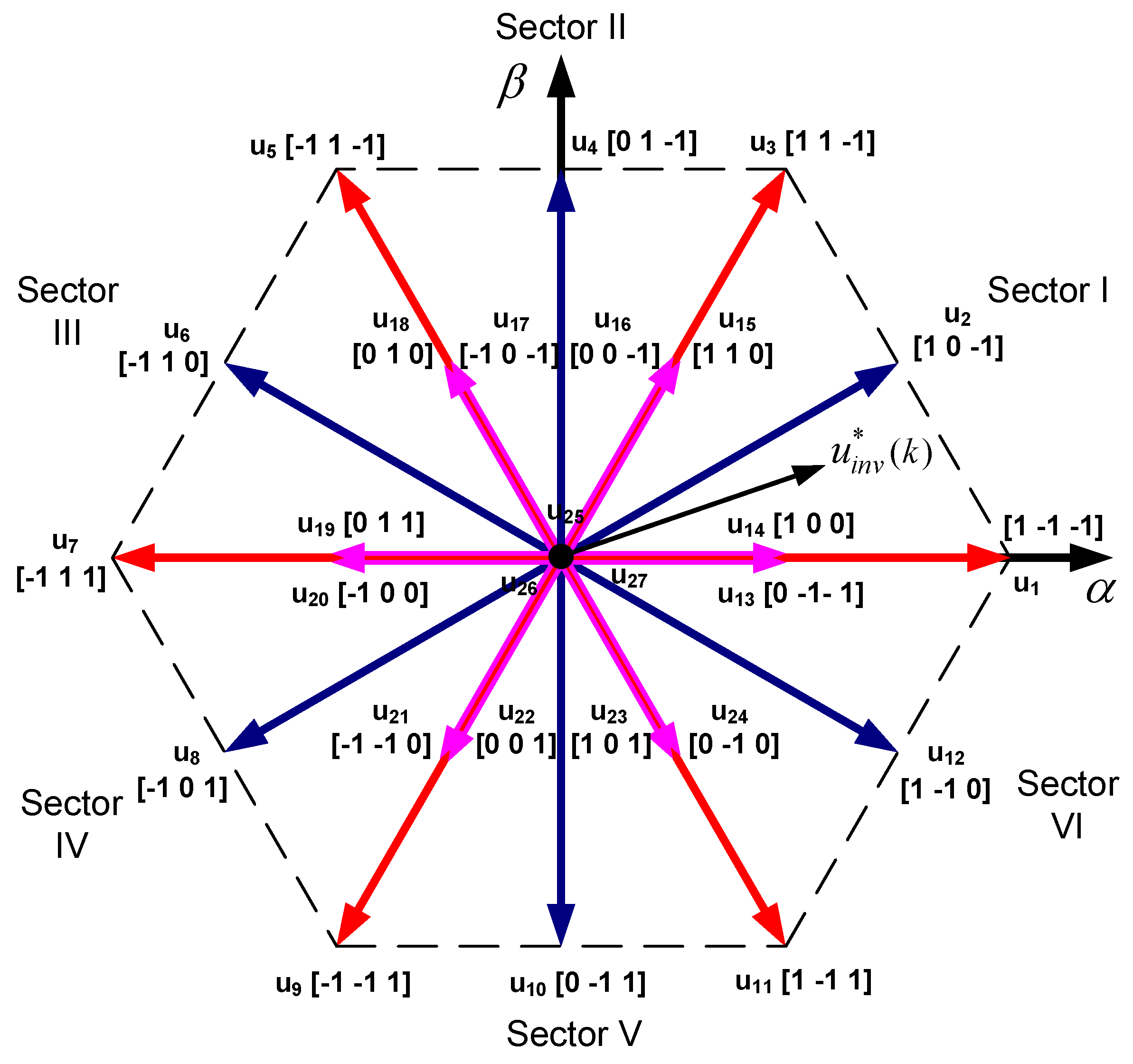
3. Model Predictive Control with Selection Sector Distribution

The main goal of the proposed control scheme is to minimize the error between the predicted output voltage and its reference value and to maintain capacitor voltage balancing. Furthermore, additional terms can be taken into account in the objective function such as switching frequency, current limitation, but this is not the main focus of this research and will not be developed here. As a result, the cost function for 3L-T-type inverter is expressed as [21,22,23]:

$$\begin{array}{c}\hfill g=\left|u_{c\alpha }^{*}(k+1)-u_{c\alpha }^p(k+1)\right|+\left|u_{c\beta }^{*}(k+1)-u_{c\beta }^p(k+1)\right|+{\lambda }_{uz}\left|u_z^p(k+1)\right|,\end{array}$$

(7)

where $u_{c\alpha }^{*}(k+1)$, $u_{c\beta }^{*}(k+1)$ and $u_{c\alpha }^p(k+1)$, $u_{c\beta }^p(k+1)$ indicate the real and imaginary components of the reference and predicted output capacitor voltages at instant $k+1$, respectively. ${\lambda }_{uz}$ is the weighting factors of the capacitor voltage balancing.

To achieve the discrete-time model, the first-order Euler approximation is used as:

$$\begin{array}{c}\hfill \frac{dx}{dt}=\frac{x(k)-x(k-1)}{T_s},\end{array}$$

(8)

where $T_s$ is the sampling time.

By approximating Equation (6) with Equation (8), the discrete-time representation of output capacitor voltage can be obtained as:

$$\begin{array}{c}\hfill u_c(k)=\frac{T_s{R}_{load}}{C_f{R}_{load}+T_s}{i}_f(k)+\frac{C_f{R}_{load}}{C_f{R}_{load}+T_s}{u}_c(k-1).\end{array}$$

(9)

By shifting the output voltage in Equation (9) into one future sample, we have the predicted output voltage at instant $k+1$:

$$\begin{array}{c}\hfill u_c^p(k+1)=\frac{T_s{R}_{load}}{C_f{R}_{load}+T_s}{i}_f^p(k+1)+\frac{C_f{R}_{load}}{C_f{R}_{load}+T_s}{u}_c(k).\end{array}$$

(10)

The discrete-time form for the filter current is given by using the forward Euler approximation as:

$$\begin{array}{c}\hfill i_f^p(k+1)=i_f(k)+\frac{T_s}{L_f}\left(u_{inv}(k)-u_c(k)\right).\end{array}$$

(11)

Similarly, the discrete-time of neutral-point potential is expressed by:

$$\begin{array}{c}\hfill u_z^p(k+1)=u_z\left(k\right)-\frac{T_s}{C}\left(\left(1-\left|S_a\right|\right)i_{fa}(k)+\left(1-\left|S_b\right|\right)i_{fb}(k)+\left(1-\left|S_c\right|\right)i_{fc}(k)\right).\end{array}$$

(12)

Substituting Equation (11) into Equation (10), the predicted output voltage is rewritten as:

$$\begin{array}{c}\hfill u_c^p(k+1)=\frac{T_s{R}_{load}}{C_f{R}_{load}+T_s}{i}_f(k)+\frac{T_s^2{R}_{load}}{L_f\left(C_f{R}_{load}+T_s\right)}{u}_{inv}(k)+\frac{R_{load}}{C_f{R}_{load}+T_s}\left(C_f-\frac{T_s^2}{L_f}\right)u_c(k).\end{array}$$

(13)

A control input is a sequential switch state $S_p={\left[S_{pa}{S}_{pb}{S}_{pc}\right]}^T$, symbolized as a set of p vector $S_p\in \left\{1,\dots ,27\right\}$. Furthermore, the switching inputs a finite set: $S_{px}\in \left\{-1,0,1\right\}$ with the index $x\in \left\{a,b,c\right\}$. As a result, the optimal switching input $S_{opt}$ is achieved as the result of Equation (14):

$$\begin{array}{cc}\hfill S_{opt}& =arg\left\{ming\right\}, p=1,\dots ,27\hfill \\ & \mathrm{subject} \mathrm{to} (7), (12) \mathrm{and} (13).\hfill \end{array}$$

(14)

The space voltage vector of 3L-T-type inverter can be classified into four groups: zero vectors (from $u_{25}$ to $u_{27}$), small vectors (from $u_{13}$ to $u_{24}$), medium vectors ($u_2$, $u_4$, $u_6$, $u_8$, $u_{10}$, and $u_{12}$) and large vectors ($u_1$, $u_3$, $u_5$, $u_7$ and $u_9$), wherein the small vectors are divided into two types: positive state (P) and negative state (N) such as $u_{14}$ and $u_{13}$, respectively. The neutral-point voltage is increased with the positive state and decreased with the negative state, respectively [33]. The zero, medium and large vectors do not affect the neutral-point voltage deviation. In the conventional FCS-MPC, the capacitor voltage balancing can be solved by adjusting the weighting factor in the cost function. However, it is not easy to obtain the optimal weighting factor value leading to affecting the THD of the load current. In this study, the capacitor voltages are balanced by selecting the suitable small vectors that depend on the predicted neutral-point voltage. Therefore, the proposed method is simple due to no requirement of the weighting factor for balancing capacitor voltages in the cost function.

For the 3L-T-type inverter, 27 switching states are considered to evaluate the cost function. Long prediction horizon can improve the control performance. However, the computational cost is increased exponentially corresponding to the prediction horizon. Therefore, it leads to a large computational cost which makes it difficult to implement the algorithm in common digital signal processing. In this paper, the selection of sector distribution is employed with the aim to solve this problem. The main idea of the proposed method is to determine the position of inverter reference voltage which is obtained from the predictive model. In this case, the required inverter voltage $u_{inv}^{*}(k)$ is achieved based on Equation (13) by replacing the predicted output voltage $u_c^p(k+1)$ with its reference. Then, the location of the reference voltage $u_{inv}^{*}(k)$ is determined by its components $u_{inv\alpha }^{*}$ and $u_{inv\beta }^{*}$. In the proposed method, we divide the space vector of the 3L T-type inverter into six sectors as illustrated in Figure 2. For example, when the reference voltage $u_{inv}^{*}(k)$ is in sector I, there are only 10 voltage vectors which are selected for the evaluation of the cost function. As previously discussed, the neutral-point voltage is predicted based on the previous optimal switching states and filter currents by using Equation (5). In order to achieve the balance of capacitor voltages, two cases are considered: the first one corresponds to $u_z\le 0$ and the second one to $u_z>0$. The positive small vectors ($u_{14}$, $u_{15}$) and negative small vectors ($u_{13}$, $u_{16}$) are considered with the condition $u_z\le 0$ and $u_z>0$, respectively. Zero vectors can reduce from 3 to 1 due to the same value and without the effect of voltage imbalance. In this case, the feasible voltage vectors are $u_1$, $u_2$, $u_3$, $u_{14}$, $u_{15}$, $u_{25}$ for $u_z\le 0$, whereas they are $u_1$, $u_2$, $u_3$, $u_{13}$, $u_{16}$, $u_{25}$ for $u_z>0$, respectively.

Table 2. Feasible voltage vectors for each sector.

Sector	Feasible Voltage Vectors
	${\mathit{u}}_{\mathit{z}}\le 0$	${\mathit{u}}_{\mathit{z}}>0$
I	$u_1$, $u_2$, $u_3$, $u_{14}$, $u_{15}$, $u_{25}$	$u_1$, $u_2$, $u_3$, $u_{13}$, $u_{16}$, $u_{25}$
II	$u_3$, $u_4$, $u_5$, $u_{15}$, $u_{18}$, $u_{25}$	$u_3$, $u_4$, $u_5$, $u_{16}$, $u_{17}$, $u_{25}$
III	$u_5$, $u_6$, $u_7$, $u_{18}$, $u_{19}$, $u_{25}$	$u_5$, $u_6$, $u_7$, $u_{17}$, $u_{20}$, $u_{25}$
IV	$u_7$, $u_8$, $u_9$, $u_{19}$, $u_{22}$, $u_{25}$	$u_7$, $u_8$, $u_9$, $u_{20}$, $u_{21}$, $u_{25}$
V	$u_9$, $u_{10}$, $u_{11}$, $u_{22}$, $u_{23}$, $u_{25}$	$u_9$, $u_{10}$, $u_{11}$, $u_{21}$, $u_{24}$, $u_{25}$
VI	$u_{11}$, $u_{12}$, $u_1$, $u_{23}$, $u_{14}$, $u_{25}$	$u_{11}$, $u_{12}$, $u_1$, $u_{24}$, $u_{13}$, $u_{25}$

illustrates the available inverter voltage vectors for a 3L-type inverter after obtaining the appropriate sector. Thus, the prediction of the control variable for cost function loop optimization is decreased from 27 to 6 with the proposed method. As a result, compared with the conventional FCS-MPC method, the computational cost is appreciably reduced by about 77% in the proposed algorithm. It is obvious that this advantage is more attractive to real-time implementation with low-cost digital hardware and long prediction horizon. The overall control strategy of the proposed method is shown in Figure 3. Then, the optimal switching state is applied to the inverter by minimizing this cost function:

$$\begin{array}{cc}\hfill g_{mdf}& =\left|u_{c\alpha }^{*}(k+1)-u_{c\alpha }^p(k+1)\right|+\left|u_{c\beta }^{*}(k+1)-u_{c\beta }^p(k+1)\right|,\hfill \\ \hfill S_{opt}& =arg\{min{g}_{mdf}\},\hspace{1em}p=1,\dots ,6.\hfill \end{array}$$

(15)

Finally, the proposed control algorithm is described in Figure 4.

4. Simulation and Experimental Results

4.1. Simulation Results

Simulation analyses were performed in a Matlab/Simulink environment with version 2015a to verify the control performance of the proposed strategy for the T-type inverter as illustrated in Figure 5. The SimPowerSystems toolbox was used to create the 3L-T-type inverter with output LC filter. The Matlab Function block is employed to easily implement the control algorithm in the simulation environment. The parameters of the system are listed in

Table 3. System parameters.

Parameter	Value	Description
$U_{dc}$	600 [V]	DC-link voltage
C	1000 [$\mathsf{\mu }$F]	DC-link capacitance
$L_f$	3 [mH]	Filter inductance
$C_f$	40 [$\mathsf{\mu }$F]	Filter capacitance
$R_{load}$	20 [$\mathsf{\Omega }$]	Load resistance
$f_s$	20 [kHz]	Sampling frequency
f	50 [Hz]	Frequency of the grid

.

Figure 6 shows the steady-state of the proposed method with the output voltage at 155 V. As depicted in Figure 6, the proposed method obtains the sinusoidal output voltage and the balance of DC-link capacitor voltage. The characteristic of the variable switching frequency is illustrated in Figure 6c. This can increase the THD of the load current, but this does not affect the control performance too much. The THD of the load current can receive further improvements by using alternative methods. However, this is not the main focus of this paper and will not be developed here.

In order to show the efficiency of the control strategy, a comparison between the proposed method and the conventional FCS-MPC [23] were carried out under different operating conditions and the same parameters. The amplitude of the reference voltage changed from 155 to 311 V in the first scenario and stepped from 311 to 155 V at $t=0.03$ s in the second scenario as illustrated in Figure 7 and Figure 8. The corresponding dynamic current response is shown in Figure 7b and Figure 8b. As can be seen, it is clear that the proposed method achieves sinusoidal current with the different reference amplitude. In addition, one important issue associated with the T-type inverter is the balance of DC-link capacitor voltage. Figure 7c and Figure 8c indicate that the voltage of the DC-link capacitor is balanced despite the change in reference. The maximum absolute error of this voltage at steady-state are about 1 and 3 V for output voltage of 155 and 311 V, respectively. Figure 9 demonstrates single phase output voltage of the proposed and conventional FCS-MPC methods. The simulation results indicate the ability of the proposed method to accurately track and accomplish the steady-state with a fast dynamic response.

With the aim to evaluate the steady-state performance, the harmonic spectra of load current for the conventional FCS-MPC and proposed methods are also examined in Figure 10a,b. These figures show that the THD of the load current is increased slightly from 0.45% to 0.58% with the proposed method. The comparison of two control methods is summarized in

Table 4. Comparison of transient performance for two controllers.

Reference Step	${\mathit{u}}_{\mathit{c}}^{*}=155\to 311$ (V)
	Conventional FCS-MPC	Proposed Method
State of loop optimization	27	6
Rise time (ms)	0.5	0.5
Settling time (ms)	0.7	1.3
THD of current (%)	0.45	0.58

. Although the THD of the load current is not perfect, we nevertheless believe that the slight increase does not affect the control performance too much. Specifically, the computation time of the proposed algorithm is greatly reduced compared with the conventional FCS-MPC as shown in Figure 11a. In fact, the minimum, average and maximum computation times of the proposed algorithm are 3, 6 and 9 $\mathsf{\mu }$s in a 2.0 GHz, i5 4310 CPU, while their corresponding values are 4, 10 and 16 $\mathsf{\mu }$s with conventional FCS-MPC. The performance of FCS-MPC method is influenced by the sampling time which is improved by choosing the smaller value. To investigate the effect of sampling time on the quality of the current, two controllers are employed with different sampling times. Figure 11b shows that the quality of load current is the best with sampling time 40 $\mathsf{\mu }$s and the worst with 100 $\mathsf{\mu }$s. However, there is a limitation of sampling time due to the requirement of execution time such as computation time and measurement of the signal. Therefore, this method exhibits a valuable alternative to reduce the sampling time and extend with a long prediction horizon, which improves the control performance.

The behavior of the system is also examined under time varying load step as illustrated in Figure 12. At the initial state, the system operates at no load condition; then, the load is set to 20 $\mathsf{\Omega }$ at $t=0.02$ s. According to Figure 12, this change does not impact on the quality of the output voltages. A resistive-inductive load is imposed for the same test as shown in Figure 13. The load resistance and inductance are set to 40 $\mathsf{\Omega }$ and 10 mH, respectively. It can be seen from Figure 13 that no deterioration of output voltage is observed in this case.

To investigate the influence of frequency variations, a step change in the voltage from 60 Hz to 50 Hz at $t=0.03$ s with $R_{load}=10$ $\mathsf{\Omega }$ is examined in this study. Figure 14 indicates that the proposed method can achieve a reasonable reference tracking despite the sudden change in the frequency.

A nonlinear load test is also performed in this study with a diode rectifier and resistive-inductive load ($R=60\mathsf{\Omega }$, $L_{nl}=10$ mH) as shown in Figure 15c. Figure 15 illustrates that the output voltages give a small distortion, but it still acquires sinusoidal in spite of the high distorted load currents.

To confirm the robustness of the controller against parameter variations, we have considered a change of parameters with two cases. In the first case, the filter inductance and capacitance have been decreased to 40% of their real values as illustrated in Figure 16a. On the other hand, the load resistance has been increased to 50% of its value as shown in Figure 16b. It can be observed that the proposed method is continued to obtain sinusoidal current with small deviations. The load current increases from 0.58% to 1.5%, but it still meets within the limit required of the IEEE 519 standard.

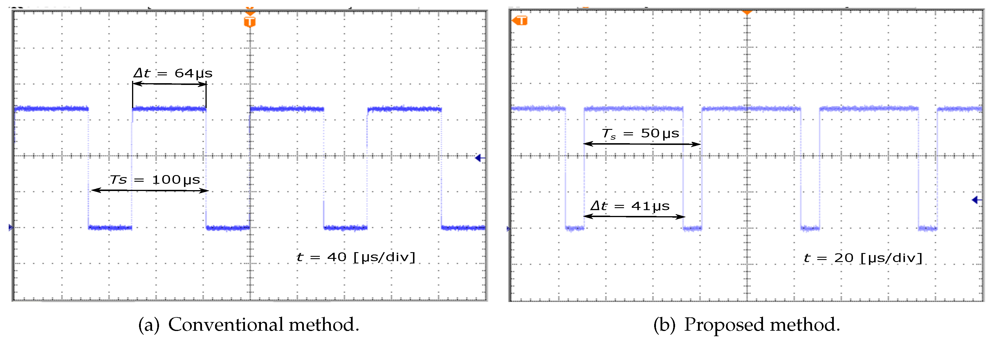
4.2. Experimental Results

In order to validate the effectiveness of the proposed control strategy, a laboratory prototype with small power was constructed as shown in Figure 17. A digital signal processor TMS320F28335 [34] was employed to implement the control method. The algorithm was programmed using S-function builder block in the Matlab/Simulink with embedded coder tools [35]. Twelves modules FGH40T120SMD for IGBT were applied in the three-phase inverter. Furthermore, two capacitors B43305A9108M 1000 $\mathsf{\mu }$F-400 V were used for DC-link voltage. The parameters of the LC filter were maintained at 3 mH and 40 $\mathsf{\mu }$F. The LV 25-P and LA 25-P sensors were used to measure the output voltage, filter current and capacitor voltages. The digital signal processing (DSP) generates the signals for 12 switches of 3L-T-type inverter via general-purpose input/output (GPIO) outputs.

The DC input voltage is set at 180 V while the load resistance is kept at 30 $\mathsf{\Omega }$. The reference of the peak phase output voltage is stepped from 90 to 60 V corresponding to the change in output current from 3 to 2 A. Figure 18 indicates that the proposed method has a fast dynamic response and a good balance of DC-link capacitor voltage. As illustrated in Figure 19, the steady-state of three-phase sinusoidal load current confirms the control performance of the proposed method. Furthermore, the execution time of the proposed and conventional FCS-MPC methods are 41 and 64 $\mathsf{\mu }$s, respectively, as shown in Figure 20. This highlights that the execution time is effectively reduced 36% by the proposed method. Therefore, the sampling time of the conventional method is increased compared with the proposed method resulting in a decrease in the quality of control performance. The load current of the conventional FCS-MPC is depicted in Figure 21. In this case, the THD of the load current of the proposed method is reduced from 1.6% to 1.0% compared with the conventional method as illustrated in Figure 22. Thus, the better performance of the proposed algorithm can be obtained with the low-cost processor.

5. Conclusions

This paper presents a simplified model predictive control method for a three-level T-type inverter. A reduced dynamics model is proposed to decrease the cost and the complexity of the system. Moreover, the execution time is greatly reduced compared with the conventional FCS-MPC by applying the preselection of reference inverter voltage and capacitor voltage balancing, allowing an easy real-time implementation. In order to show the effectiveness of the control strategy, a comparative study of the proposed method and conventional FCS-MPC is performed. Simulation and experimental results prove the feasibility of the proposed approach.

References

1. Blaabjerg, F.; Liserre, M.; Ma, K. Power Electronics Converters for Wind Turbine Systems. IEEE Trans. Ind. Appl. 2012, 48, 708–719. [Google Scholar] [CrossRef]
2. Portillo, R.C.; Prats, M.M.; Leon, J.I.; Sanchez, J.A.; Carrasco, J.M.; Galvan, E.; Franquelo, L.G. Modeling Strategy for Back-to-Back Three-Level Converters Applied to High-Power Wind Turbines. IEEE Trans. Ind. Electron. 2006, 53, 1483–1491. [Google Scholar] [CrossRef]
3. Kouro, S.; Malinowski, M.; Gopakumar, K.; Pou, J.; Franquelo, L.G.; Wu, B.; Rodriguez, J.; Perez, M.A.; Leon, J.I. Recent Advances and Industrial Applications of Multilevel Converters. IEEE Trans. Ind. Electron. 2010, 57, 2553–2580. [Google Scholar] [CrossRef]
4. Schweizer, M.; Kolar, J.W. Design and Implementation of a Highly Efficient Three-Level T-Type Converter for Low-Voltage Applications. IEEE Trans. Power Electron. 2013, 28, 899–907. [Google Scholar] [CrossRef]
5. Lee, K.; Shin, H.; Choi, J. Comparative analysis of power losses for 3-Level NPC and T-type inverter modules. In Proceedings of the 2015 IEEE International Telecommunications Energy Conference (INTELEC), Osaka, Japan, 18–22 October 2015; pp. 1–6. [Google Scholar]
6. Qin, C.; Zhang, C.; Chen, A.; Xing, X.; Zhang, G. A Space Vector Modulation Scheme of the Quasi-Z-Source Three-Level T-Type Inverter for Common-Mode Voltage Reduction. IEEE Trans. Ind. Electron. 2018, 65, 8340–8350. [Google Scholar] [CrossRef]
7. Vahedi, H.; Labbe, P.A.; Al-Haddad, K. Balancing three-level NPC inverter DC bus using closed-loop SVM Real time implementation and investigation. IET Power Electron. 2016, 9, 2076–2084. [Google Scholar] [CrossRef]
8. Xiang, C.; Shu, C.; Han, D.; Mao, B.; Wu, X.; Yu, T. Improved Virtual Space Vector Modulation for Three-Level Neutral-Point-Clamped Converter With Feedback of Neutral-Point Voltage. IEEE Trans. Power Electron. 2018, 33, 5452–5464. [Google Scholar] [CrossRef]
9. Ngo, B.Q.V.; Ayerbe, P.R.; Olaru, S. Model Predictive Control with Two-step horizon for Three-level Neutral-Point Clamped Inverter. In Proceedings of the 20th International Conference on Process Control, Strbske Pleso, Slovakia, 9–12 June 2015; pp. 215–220. [Google Scholar]
10. In, H.C.; Kim, S.M.; Lee, K.B. Design and Control of Small DC-Link Capacitor-Based Three-Level Inverter with Neutral-Point Voltage Balancing. Energies 2018, 11, 1435. [Google Scholar] [CrossRef]
11. Wilamowski, B.M.; Irwin, J.D. Power Electronics and Motor Drives; Taylor and Francis Group: Boca Raton, FL, USA, 2011. [Google Scholar]
12. Zorig, A.; Belkheiri, M.; Barkat, S. Control of three-level T-type inverter based grid connected PV system. In Proceedings of the 13th International Multi-Conference on Systems, Leipzig, Germany, 21–24 March 2016; pp. 66–71. [Google Scholar]
13. Malinowski, M.; Kazmierkowski, M.P.; Hansen, S.; Blaabjerg, F.; Marques, G.D. Virtual-flux-based direct power control of three-phase PWM rectifiers. IEEE Trans. Ind. Appl. 2001, 37, 1019–1027. [Google Scholar] [CrossRef]
14. Malinowski, M.; Jasinski, M.; Kazmierkowski, M.P. Simple direct power control of three-phase PWM rectifier using space-vector modulation (DPC-SVM). IEEE Trans. Ind. Electron. 2004, 51, 447–454. [Google Scholar] [CrossRef]
15. Farahani, H.F.; Rashidi, F. Direct power control of a grid-connected photovoltaic system using a fuzzy-logic based controller. Simul.-Trans. Soc. Model. Simul. Int. 2017, 93, 213–223. [Google Scholar] [CrossRef]
16. Sebaaly, F.; Vahedi, H.; Kanaan, H.Y.; Moubayed, N.; Al-Haddad, K. Design and Implementation of Space Vector Modulation-Based Sliding Mode Control for Grid-Connected 3L-NPC Inverter. IEEE Trans. Ind. Electron. 2016, 63, 7854–7863. [Google Scholar] [CrossRef] [Green Version]
17. Donoso, F.; Mora, A.; Cárdenas, R.; Angulo, A.; Sáez, D.; Rivera, M. Finite-Set Model-Predictive Control Strategies for a 3L-NPC Inverter Operating With Fixed Switching Frequency. IEEE Trans. Ind. Electron. 2018, 65, 3954–3965. [Google Scholar] [CrossRef]
18. Vazquez, S.; Mohan, C.; Franquelo, L.G.; Marquez, A.; Leon, J.I. A Generalized Predictive control for T-type power inverters with output LC filter. In Proceedings of the 9th International Conference on Compatibility and Power Electronics (CPE), Costa da Caparica, Portugal, 24–26 June 2015; pp. 20–24. [Google Scholar]
19. Nauman, M.; Hasan, A. Efficient Implicit Model-Predictive Control of a Three-Phase Inverter With an Output LC Filter. IEEE Trans. Power Electron. 2016, 31, 6075–6078. [Google Scholar] [CrossRef]
20. Xing, X.; Chen, A.; Zhang, Z.; Chen, J.; Zhang, C. Model predictive control method to reduce common-mode voltage and balance the neutral-point voltage in three-level T-type inverter. In Proceedings of the IEEE Applied Power Electronics Conference and Exposition, Long Beach, CA, USA, 20–24 March 2016; pp. 3453–3458. [Google Scholar]
21. Kouro, S.; Cortes, P.; Vargas, R.; Ammann, U.; Rodriguez, J. Model Predictive Control:A Simple and Powerful Method to Control Power Converters. IEEE Trans. Ind. Electron. 2009, 56, 1826–1838. [Google Scholar] [CrossRef]
22. Rodriguez, J.; Kazmierkowski, M.P.; Espinoza, J.R.; Zanchetta, P.; Abu-Rub, H.; Young, H.A.; Rojas, C.A. State of the Art of Finite Control Set Model Predictive Control in Power Electronics. IEEE Trans. Ind. Inf. 2013, 9, 1003–1016. [Google Scholar] [CrossRef]
23. Rodriguez, J.; Cortes, P. Predictive Control of Power Converters and Electrical Drives; John Wiley: New York, NY, USA, 2012. [Google Scholar]
24. Ngo, B.Q.V.; Rodriguez-Ayerbe, P.; Olaru, S.; Niculescu, S.I. Model predictive power control based on virtual flux for grid connected three-level neutral-point clamped inverter. In Proceedings of the 18th European Conference on Power Electronics and Applications, Karlsruhe, Germany, 5–9 September 2016; pp. 1–10. [Google Scholar]
25. Singh, V.K.; Tripathi, R.N.; Hanamoto, T. HIL Co-Simulation of Finite Set-Model Predictive Control Using FPGA for a Three-Phase VSI System. Energies 2018, 11, 909. [Google Scholar] [CrossRef]
26. Shi, T.; Zhang, C.; Geng, Q.; Xia, C. Improved model predictive control of three-level voltage source converter. Electr. Power Compon. Syst. 2014, 42, 1029–1138. [Google Scholar] [CrossRef]
27. Xia, C.; Liu, T.; Shi, T.; Song, Z. A Simplified Finite-Control-Set Model-Predictive Control for Power Converters. IEEE Trans. Ind. Inf. 2014, 10, 991–1002. [Google Scholar]
28. Geyer, T.; Quevedo, D.E. Performance of Multistep Finite Control Set Model Predictive Control for Power Electronics. IEEE Trans. Power Electron. 2015, 30, 1633–1644. [Google Scholar] [CrossRef]
29. Aguilera, R.P.; Baidya, R.; Acuna, P.; Vazquez, S.; Mouton, T.; Agelidis, V.G. Model predictive control of cascaded H-bridge inverters based on a fast-optimization algorithm. In Proceedings of the 41st Annual Conference of the IEEE Industrial Electronics Society, Yokohama, Japan, 9–12 November 2015; pp. 4003–4008. [Google Scholar]
30. Liu, X.; Wang, D.; Peng, Z. Improved finite-control-set model predictive control for active front-end rectifiers with simplified computational approach and on-line parameter identification. ISA Trans. 2017, 69, 51–64. [Google Scholar] [CrossRef] [PubMed]
31. Zhang, Z.; Hackl, C.M.; Kennel, R. Computationally Efficient DMPC for Three-Level NPC Back-to-Back Converters in Wind Turbine Systems With PMSG. IEEE Trans. Power Electron. 2017, 32, 8018–8034. [Google Scholar] [CrossRef]
32. Taheri, A.; Zhalebaghi, M.H. A new model predictive control algorithm by reducing the computing time of cost function minimization for NPC inverter in three-phase power grids. ISA Trans. 2017, 71, 391–402. [Google Scholar] [CrossRef] [PubMed]
33. Wu, B.; Narimani, M. High-Power Converters and AC Drives; Wiley-IEEE Press: New York, NY, USA, 2017. [Google Scholar]
34. TMS320F28335 controlCARD. Available online: http://www.ti.com/tool/tmdscncd28335 (accessed on 28 October 2018).
35. Elrajoubi, A.; Ang, S.S.; Abushaiba, A. TMS320F28335 DSP programming using MATLAB Simulink embedded coder: Techniques and advancements. In Proceedings of the 2017 IEEE 18th Workshop on Control and Modeling for Power Electronics (COMPEL), Stanford, CA, USA, 9–12 July 2017; pp. 1–7. [Google Scholar]
Figure 1. Three-level T-type inverter topology.
Energies 12 00031 g001
Figure 2. Voltage vectors distribution of T-type inverter.
Energies 12 00031 g002
Figure 3. Block diagram of the proposed control strategy.
Energies 12 00031 g003
Figure 4. Flowchart of the proposed control strategy.
Energies 12 00031 g004
Figure 5. Block diagram of the proposed strategy in Matlab/Simulink.
Energies 12 00031 g005
Figure 6. Steady-state of the proposed method at the output voltage of 155 V.
Energies 12 00031 g006
Figure 7. The dynamic response of the proposed method for step change from 311 to 155 V.
Energies 12 00031 g007
Figure 8. The dynamic response of the proposed method for step change from 155 to 311 V.
Energies 12 00031 g008
Figure 9. The dynamic response of the output voltage for the conventional FCS-MPC and proposed methods.
Energies 12 00031 g009
Figure 10. The harmonic spectrum of the load current for the conventional FCS-MPC and proposed methods.
Energies 12 00031 g010
Figure 11. Comparison of two control methods.
Energies 12 00031 g011
Figure 12. Output voltage and current with the resistive load step at t = 0.02 s.
Energies 12 00031 g012
Figure 13. Output voltage and current with the resistive–inductive load step at t = 0.02 s.
Energies 12 00031 g013
Figure 14. The output voltage and current responses under dynamic change in frequency.
Energies 12 00031 g014
Figure 15. Output voltage and current with nonlinear load.
Energies 12 00031 g015
Figure 16. Output current with parameter variations.
Energies 12 00031 g016
Figure 17. Experimental test bench in the laboratory.
Energies 12 00031 g017
Figure 18. Experimental results for step change in the output voltage.
Energies 12 00031 g018
Figure 19. Experimental results of the proposed method with I f = 3 A.
Energies 12 00031 g019
Figure 20. Execution time of the conventional and proposed methods.
Energies 12 00031 g020
Figure 21. Experimental results of the conventional FCS-MPC.
Energies 12 00031 g021
Figure 22. THD of load current.
Energies 12 00031 g022