Online Recognition Method for Voltage Sags Based on a Deep Belief Network

Abstract

Voltage sag is a serious power quality phenomenon that threatens industrial manufacturing and residential electricity. A large-scale monitoring system has been established and continually improved to detect and record voltage sag events. However, the inefficient process of data sampling cannot provide valuable information early enough for governance of the system. Therefore, a novel online recognition method for voltage sags is proposed. The main contributions of this paper include: 1) The causes and waveform characters of voltage sags were analyzed; 2) according to the characters of different sag waveforms, 10 voltage sag characteristic parameters were proposed and proven to be effective; 3) a deep belief network (DBN) model was built using these parameters to complete automatic recognition of the sag event types. Experiments were conducted using voltage sag data from one month recorded by the 10 kV monitoring points in Suqian, Jiangsu Province, China. The results showed good performance of the proposed method: Recognition accuracy was 96.92%. The test results from the proposed method were compared to the results from support vector machine (SVM) recognition methods. The proposed method was shown to outperform SVM.

1. Introduction

Voltage sags are the unavoidable short-term disturbances in the operation of a power system. The root mean square (RMS) value of voltage suddenly drops and recovers after a short time. The institute of electrical and electronics engineers (IEEE) definition for voltage sag is as follows: the RMS voltage drops to 10%–90% of the rated value, and the duration is 10 ms–60 s [1,2]. Significant negative impacts on society and tremendous economic losses in industrial production have been caused by voltage sags [3,4,5]. In 2010, a production process was interrupted as a result of the abnormal operation of the frequency converter because of voltage sag in a cigarette factory in Xuzhou, Jiangsu Province, China. In 2014, power outages of electrical lines occurred as a result of the low voltage trip of distribution switches because of voltage sag in the Nanjing south railway station, Jiangsu Province. With the continual expansion of power systems and the increase in voltage levels, various types of electronic and electrical equipment have become increasingly connected to the power grid. Traditional equipment, including computers, frequency converters, programmable logic controllers (PLCs), and alternating current (AC) contactors, as well as new equipment developed in recent years such as renewable energy generation systems with power electronics as the core, are sensitive to voltage sag disturbances [6,7]. Therefore, the research and treatment of voltage sags are important in improving the reliability of power systems and ensuring a power supply in industrial production and daily life. At present, data collection, detection, classification, and identification of voltage sags are the focus of research [8,9,10,11,12].

As an important part of the power quality index system, voltage sag is the key to a high-quality power supply [13]. The monitoring and analysis of voltage sag events can provide an effective scientific basis for power system operations management, accident investigation, fault location, and sag management. In Jiangsu Province, a voltage sag online monitoring system and big data platform have been established since 2016. At present, more than 17,000 monitoring points have been accessed. The monitoring voltage level is 10–500 kV. This online monitoring system has been established in strict accordance with the requirements of the international standard IEC 61000-4-30:2008. A large amount of original sampling data collected by the monitoring system is stored in this big data platform. These data completely record the transient waveforms of each detected sag event for further data analysis and mining. However, the efficiency of this data analysis is low because of a lack of effective data processing means. Therefore, two main problems must be addressed. On the one hand, voltage sag events are manually identified and classified. Specifically, operation and maintenance engineers analyze the RMS waveform of the voltage sag, assess the detriment, and confirm the type and reason. The results heavily depend on the skills and experience of field engineers. On the other hand, it is difficult for the big data platform to save a massive amount of data. Larger amounts of data that are difficult to process in time may be discarded, or decrease in value, resulting in a waste of resources. Thus, it is difficult for voltage sag data analysis and processing technology to keep pace with the development of the monitoring system. Moreover, this gap will further widen with the expansion of the monitoring system and improvements in sampling precision.

The pattern recognition of voltage sags is the premise for locating disturbance sources and the basis of sag management. Many studies have been performed in this context. In general, there are three methods: Physical modeling, signal processing, and data mining. Physical modeling is useful for understanding the mechanism of voltage sags. In Reference [14], Thevenin’s equivalent circuit was used to replace any power network. By determining the sign of the internal resistance in Thevenin’s equivalent circuit, the origin of a voltage sag disturbance could be easily identified. Signal processing achieves recognition by extracting the characteristics of a sag waveform. In Reference [15], a method for voltage sag source identification that combined wavelet analysis and modified dynamic time warping (DTW) distance was proposed. Reference [16] introduced a new voltage sag index, “S”, for the joint characterization of voltage sags and swell conditions. In Reference [17], a statistical analysis of variance (MANOVA) was directly proposed to extract the attributes of voltage events from the voltage and current waveforms. The most relevant attributes have been used as the input for rule-extraction algorithms to extract classification rules. In recent years, data mining and artificial intelligence have been research hotspots and have proven to be an effective means in this respect. These areas represent an important development direction for high-achieving efficiency and precision. K-means clustering was used to identify voltage sag in Reference [18]. A support vector machine (SVM) and support vector regression (SVR) were used to identify fault types and estimate fault resistance. The Euclidean distance approach was used to identify the fault distance in Reference [19]. Reference [20] detected and classified different power quality disturbances using the half- and one-cycle windowing technique (WT) based on a continuous S-transform (CST) and neural network (NN). Reference [21] proposed a Kullback-Leibler (KL) divergence measure and standard deviation for voltage sag and harmonics identification.

Data mining and artificial intelligence techniques offer three advantages in classifying and identifying voltage sag events. First, effective information can be extracted from massive data, which contributes to the in-depth understanding of the universal law of voltage sags. Second, scientific and effective technical support can be provided for voltage sag management, power grid upgrading, reconstruction, and access design of sensitive users. Third, the techniques can provide new ideas for solving other power quality problems. In this paper, a new index system, including 10 characteristic parameters and a deep belief network (DBN)-based online voltage sag recognition model, are proposed, which can provide a reliable solution for data processing and automatic recognition. First, the typical transient waveforms of various voltage sags (including single-phase short circuit, two-phase short circuit, three-phase short circuit, induction motor starting, and transformer energizing) were analyzed, and the mechanism and differences between various voltage sags were clarified. Second, the 10 voltage sag characteristic parameters were calculated using the formulas reported in this paper. Finally, a DBN-based voltage sag recognition model was established with these characteristic parameters. The characteristic parameters formed the basis for establishing the recognition model, and the differentiation of parameters was beneficial in improving the recognition accuracy. In this paper, the characteristic parameters were derived from the graphical features of the voltage sag waveform, and the calculation method was simple. The DBN is a useful tool in the field of pattern recognition and fault diagnosis [22,23,24,25]. As a type of deep learning neural network, compared to the traditional artificial neural network (ANN), DBNs can be used for unsupervised learning [26,27]. Automatic coding can be achieved through a large amount of data training, and the shortcoming of relying too heavily on data labels is overcome. Moreover, the accuracy of a DBN classifier can be improved by fine-tuning using a small number of tagged samples. The performance of the characteristic index and DBN recognition model was verified using voltage sag data recorded by the 10 kV monitoring points in Suqian, Jiangsu Province. The results demonstrated that first, the 10 voltage sag characteristic parameters proposed in this paper were reasonable. They had good aggregation of identical category features and decentralization of different category features. Second, the accuracy of the DBN model was 96.92%, which was higher than that of the traditional recognition model SVM, and the requirements for sample labels were lower, which was more suitable for online recognition. Third, the DBN model included offline and online modules. A large number of training processes were completed by the off-line module, and the online module only performed identification of new samples. The efficiency was high. The method proposed in this paper provides a new solution for the automatic recognition of voltage sags. Accurate and efficient recognition results provide a reliable scientific basis in time for the management of voltage sag.

The rest of this paper is organized as follows. In Section 2, waveforms and features of different kinds of voltage sags are analyzed. The 10 voltage sag characteristic parameters and their calculation methods are proposed in Section 3. In Section 4, the theory of DBN modeling and voltage sag recognition methods are presented. In Section 5, some actual data are used to verify the effectiveness of the characteristic parameters and DBN recognition model. Conclusions are drawn in Section 6.

2. Analysis of Voltage Sags

At present, voltage sag problems in power systems are derived from two main sources, short-circuit faults and the starting or energizing of high-capacity electrical equipment. Short-circuit faults include single-phase short circuits, two-phase short circuits, and three-phase short circuits. High-capacity equipment includes high-capacity motor and capacitors. Different voltage sag sources show distinct electrical characteristics. In general, the transient processes of short-circuit faults are short, whereas those associated with starting or energizing electrical equipment are long. Finding the relationship between voltage sag sources and electrical characteristics is the basis for establishing a reasonable classification and recognition model. Analysis of the cause of the voltage sags and the voltage waveform characteristics for each type of sag events are prerequisites for proposing reasonable parameters.

2.1. Short-Circuit Faults

Short circuits represent a serious fault in a power system. Voltage sags are inevitably caused by the spread of short-circuit currents in adjacent lines. Sag degree and sag time are directly related to the fault type, fault location, monitoring point location, short-circuit impedance, and protection strategy. Finding the correlation between disturbance sources and the associated electrical characteristics is the basis for establishing a scientific and rational recognition model. Figure 1a–c shows the typical waveforms of the voltage RMS in the case of a single-phase short-circuit fault (A phase, B phase, and C phase, respectively). Figure 2a–c shows typical waveforms of the voltage RMS in the case of a two-phase short-circuit fault (A- and B-phases, B- and C-phases, and A- and C-phases). Figure 3 shows the typical waveforms of the voltage RMS in the case of a three-phase short-circuit fault.

The figures illustrate the following:

• The falling and rising parts of the curve are steep. Therefore, the generating process and recovery process of voltage sags caused by a short-circuit fault are short, occurring at high speed.
• In the voltage sag interval, all waveform shapes are rectangular. Moreover, the sag amplitude essentially remains stable.
• The depth of voltage sag is low relatively, and the duration is related to the operating time of short-circuit protection.
• The voltage amplitude of the fault phase decreases significantly, whereas the non-fault phase remains stable or slightly drops. In some cases, voltage swells appear in a non-fault phase.

2.2. The Starting or Energizing of High-Capacity Electrical Equipment

Induction motors are important loads, and large transformers are key devices in the power grid. When a motor starts or a no-load transformer energizes, the excitation current can reach 5–7 times the working current. An obvious voltage sag can be observed at the point of common coupling (PCC) after the large current flow through system impedance. This type of voltage sag gradually recovers to normal when the starting or energizing process completes. Compared to that of the sag caused by a short-circuit fault, the excitation current is smaller. Moreover, the time required for the starting or energizing is longer. Therefore, the waveform characteristics between these two voltage sag sources are significantly different. Figure 4 and Figure 5 show the typical waveforms of the voltage RMS in the cases of a motor starting and a transformer energizing.

The figures illustrate the following:

• The waveform shapes of voltage sags are not obviously rectangular. The voltage quickly drops at the beginning of the sag and recovers slowly. The shape is closer to triangular.
• Since the excitation current is much smaller than the short-circuit current, the voltage sag depth associated with starting or energizing a high-capacity electrical equipment is small. Moreover, the depth of motor starting is determined by the motor starting capacity and upper transformer capacity. Furthermore, the depth of the transformer energizing is related to self-capacity.
• The recovery processes associated with a motor starting and a transformer energizing are essentially identical, although there are differences at the beginning of the voltage sag.

3. Characteristics of Voltage Sag

Data pertaining to characteristics of interest are the raw materials for data mining and machine learning. Therefore, the features should contain as much effective information about a voltage sag event as possible. The selection of features should follow three principles. First, features with the same categories are concentrated. The features should be approximate if they belong to the same voltage sag event. Second, features of different categories are decentralized. There should be significant differences among the features of different voltage sag events. Third, the calculation process should be relatively simple. Traditionally, voltage sag data are manually processed. The voltage RMS waveform is important and can be analyzed for recognition and diagnosis of voltage sag events. This mode is a reliable solution in the processing of a small number of data samples. Therefore, the processing efficiency is low when one processes massive data samples.

Generally, the voltage RMS is expressed as follows [28]:

$$U_{RMS}(i)=\sqrt{\frac{1}{N}{\displaystyle \sum _{i+1-N/2}^{i+N/2}{u}^2(i)}}$$

(1)

where U_RMS(i) is the voltage RMS of the discrete voltage signal u(i), i is the sampling point, and N is the number of sampling points in one cycle. In this paper, a voltage sag feature system with 10 parameters is proposed according to the waveform characteristic. These parameters were calculated using the voltage RMS, which are described in detail as follows.

3.1. Descending or Ascending Velocities of Three-Phase Voltages $Ve{l}_A$, $Ve{l}_B$, and $Ve{l}_C$

The velocity of the voltage decrease or increase is the slope of the falling or rising section of the voltage RMS waveform, as shown in Figure 6a. The descending velocity of the motor starting is less than that of other types of voltage sag. Therefore, these parameters can be used to distinguish the motor starting voltage sag. Moreover, the decrease or increase in voltage can be used to confirm the fault phase of a short circuit. For example, in Figure 1a, $Ve{l}_A$ is the velocity of the A-phase and is negative; and $Ve{l}_B$ and $Ve{l}_C$ are the velocities of the B- and C-phases, respectively, and are positive. These results show that there is a short circuit in the A-phase.

To eliminate interference and ensure the stability of data calculation, in this paper, the calculation interval was set as the middle 80% part within the distance from the sag start point to the sag end point. The calculation formula was as follows:

$$Vel=\frac{0.1U_{sag}-0.9U_{sag}}{i_2^{\prime }-i_1^{\prime }}$$

(2)

where $i_1^{\prime }$ and $i_2^{\prime }$ are the times when the voltage dropped to 0.9 U_sag and 0.1 U_sag, respectively; $U_{sag}=U_{\max }-U_{\min }$; and $U_{\max }$ and $U_{\min }$ are the maximum and minimum voltages, respectively.

3.2. Recovery Velocities of Three-Phase Voltages $Re{s}_A$, $Re{s}_B$, and $Re{s}_C$

The recovery process is the inverse of voltage sag or swell. After a certain time, the voltage RMS returns to normal because the short-circuit fault is eliminated and the high-capacity electrical equipment finishes starting or energizing. However, the recovery procedure of different voltage sags varies. In Figure 1, Figure 2, Figure 3, Figure 4 and Figure 5, the recovery procedure of the short-circuit fault is short, and the voltage recovery slopes $Re{s}_A$, $Re{s}_B$, and $Re{s}_C$ are larger. The recovery procedure associated with starting or energizing high-capacity electrical equipment is long, and the voltage recovery slope is small. These parameters are important references for identifying short-circuit voltage sag events. Similarly, the recovery velocity is defined as the average slope of the middle 80% part of the voltage recovery process, as shown in Figure 6a:

$$Res=\frac{0.9U_{sag}-0.1U_{sag}}{i_2^{″}-i_1^{″}}$$

(3)

where $i_1^{″}$ and $i_2^{″}$ are the times when the voltage recovered to 0.1 U_sag and 0.9 U_sag, respectively.

3.3 Non-Rectangular Coefficients $Re{c}_A$, $Re{c}_B$, and $Re{c}_C$

Because the process of sag occurrence and recovery is short, the speeds at which the voltage drops and rises are large. Moreover, the voltage is essentially stable during the sag. Therefore, the voltage RMS waveform is approximately rectangular in the short-circuit fault. However, the sag waveform associated with the starting or energizing of high-capacity electrical equipment is more triangular in shape. Hence, nonrectangular coefficients are also important parameters in the identification of short-circuit faults. In this paper, the nonrectangular coefficient was defined as the ratio of the sum of the deviation degrees of $U_{RMS}(i)$ to the deviation degrees of $U_{\min }$ in the complete sag interval, as shown in Figure 6b:

$$Rec=\frac{{\displaystyle \sum _{i=i_1}^{i_2}(0.9-U_{RMS}(i))}}{(0.9-U_{\min })(i_2-i_1)}$$

(4)

where $i_1$ and $i_2$ are the starting time and ending time of the voltage sag interval, respectively. In other words, $i_1$ and $i_2$ are the times when the voltage drops to 0.9 pu and recovers to 0.9 pu. An Rec value close to 1 indicates a highly rectangular sag waveform.

3.4. Three-Phase Voltage Unbalance Ratio (PVUR)

The three-phase voltage unbalance ratio is an effective parameter for distinguishing among different types of short-circuit faults and determining the short-circuit phase. Motor starting, transformer energizing, and three-phase short-circuit faults have relatively low PVUR values, while single-phase and two-phase short-circuit faults have higher PVUR values. The PVUR calculation method defined in IEEE Std 112-2004 was adopted in this paper:

$$\mathrm{PVUR}=\frac{\max \left[|V_a-V_{avg}|, |V_b-V_{avg}|, |V_c-V_{avg}|\right]}{V_{avg}}\times 100\%$$

(5)

where $V_a$, $V_b$, and $V_c$ are the phase voltage effective values and $V_{avg}$ is the average value of the three phase voltages.

4. Recognition Process of a Deep Belief Network

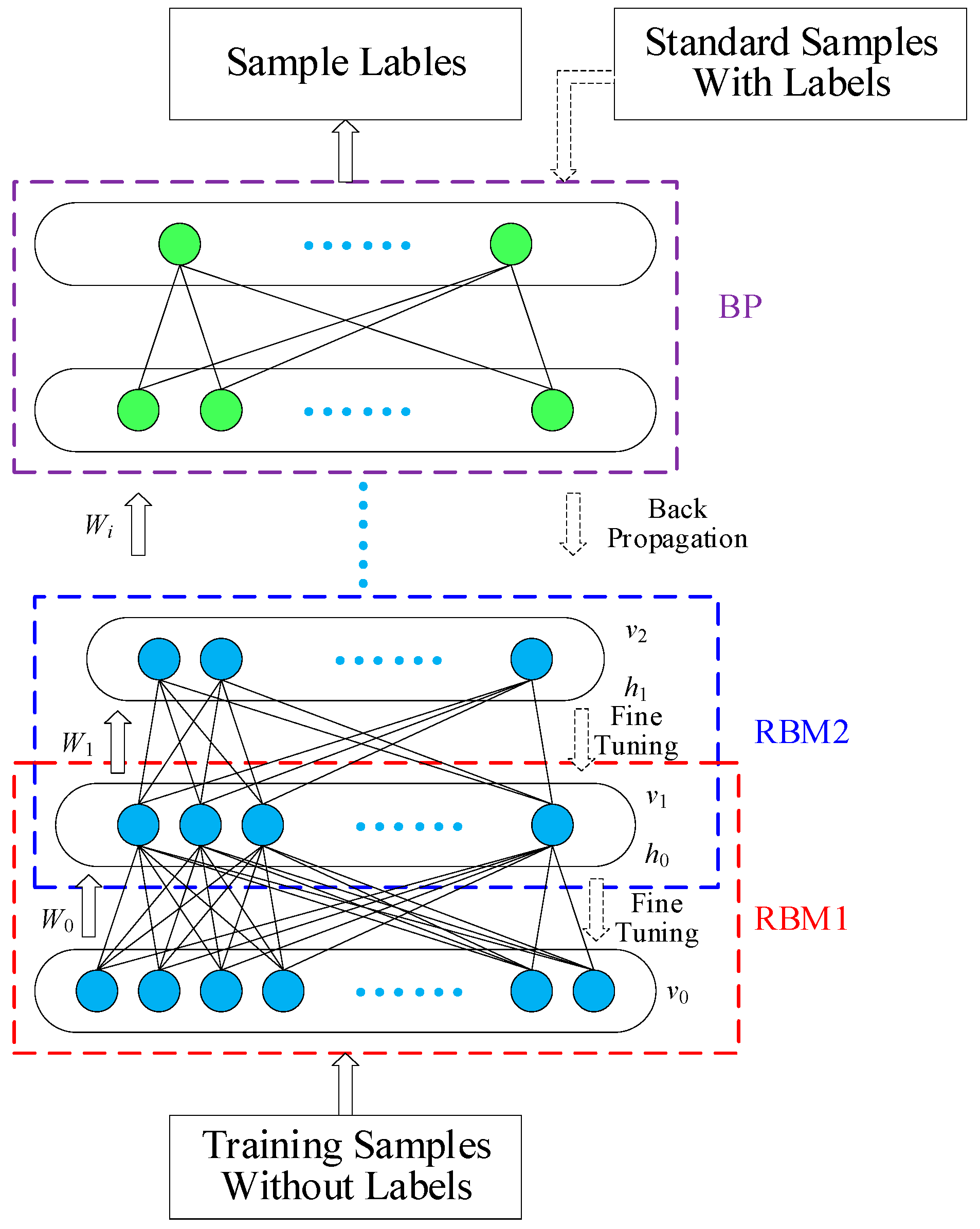
4.1. Modeling principle of DBNs

A DBN is composed of multilayer neurons, and the component is the restricted Boltzmann machine (RBM). The RBM is a neural perceptron consisting of a visible layer and a hidden layer. The neurons of the visible layer and hidden layer are bidirectionally connected, and there is no connection among the neurons in the same layer. The visible layer is used as the data input, and the hidden layer is used for feature extraction. The output data of the low-level RBM is used as the input sample of the high-level RBM. The RBM overall energy of the visible layer variable $\nu$ and hidden layer variable $h$ is defined as [29]:

$$E(v,h|\theta )=-v^{\mathrm{T}}Wh-a^{\mathrm{T}}v-b^{\mathrm{T}}h=-{\displaystyle \sum _{i=1}^m{\displaystyle \sum _{j=1}^n{W}_{ij}{h}_i{v}_j}}-{\displaystyle \sum _{j=1}^n{a}_j{v}_j}-{\displaystyle \sum _{i=1}^m{b}_i{h}_i}$$

(6)

where $\nu$ is the state vector of the visible layer node; $h$ is the state vector of the hidden layer node; m and n are the numbers of visible layer nodes and hidden layer nodes, respectively; W is the connection weight of the visible layer node and hidden layer node; and $\theta =\left\{W,a,b\right\}$ are the parameters of the RBM model, where a and b are the offset values of the visible layer nodes and hidden layer nodes, respectively. Figure 7 is a typical DBN architecture.

According to the Boltzmann distribution function, if parameters $\theta =\left\{W,a,b\right\}$ are confirmed, the joint probability distribution of $(\nu ,h)$ can be calculated by the following equations, where Z is the partition equation:

$$P(v,h|\theta )=\frac{e^{-E(v,h|\theta )}}{Z(\theta )}$$

(7)

$$Z(\theta )=-{\displaystyle \sum _{v,h}{e}^{-E(v,h|\theta )}}$$

(8)

The probability that the network assigns to a visible layer node is

$$p(v)=\frac{1}{Z}{\displaystyle \sum _h{e}^{-E(v,h|\theta )}}$$

(9)

If each node state of the visible layer and the hidden layer is known, the conditional probability function of the hidden layer node or visible layer node can be separately obtained. The probability that the binary state of the node is set to 1 is:

$$p(h_i=1|v)=\sigma (b_i+\sum _{j=1}^n{w}_{ij}{v}_j)$$

(10)

$$p(v_i=1|h)=\sigma (a_j+\sum _{i=1}^m{w}_{ij}{h}_i)$$

(11)

where $\sigma (x)$ is the sigmoid function $\sigma (x)=1/(1+e^{-x})$.

In this paper, a contrastive divergence (CD-k) algorithm was used to determine the RBM parameters $\theta =\left\{W,a,b\right\}$. The layer-by-layer training mechanism was used to train the visible layer and hidden layer of a certain RBM layer at a time, and the optimal parameters of this layer could be obtained. Moreover, feature extraction was completed on the current layer. Subsequently, the output data were continuously used as the input samples of the next RBM layer to be trained. The entire DBN was greedily trained layer by layer. A back propagation (BP) algorithm was used for parameter fine-tuning using some samples with category labels. Traditionally, the network weights and offsets are initialized using random values. In this paper, the weights and offsets were replaced by the weights obtained from the pre-training of the multilayer RBM. In this process, a BP network was set as a classifier on the top layer of the DBN. The output data of the RBM were the input of the BP network, and supervised training was executed to obtain the error. Then, the error was propagated from the top layer to every RBM layer to adjust the network parameters.

4.2. Voltage Sag Recognition Model Based on a DBN

In this paper, the training and testing data were collected by an online monitoring system. When a voltage sag event occurred, the sampling data were recorded, and the characteristic parameters were calculated. Then, the DBN model was automatically established for classification and recognition. This model included two parts, an offline modeling module and an online recognition module. The offline module used historical data, and the online module used real-time data. The offline modeling module could realize the preprocessing and feature extraction of historical data and the training of the DBN. These raw sampling data were transformed into a feature matrix as a training set for the DBN. Then, the training of the DBN model was completed. In the online recognition module, new unrecognized sag data from the online monitoring system were processed to obtain the characteristic parameters, and these parameters were input into the DBN for recognition. The category labels of these new voltage sag data were obtained, and the recognition process finished. Furthermore, these new sag data were supplemented as the new training data for the DBN in the historical database, which was confirmed without errors. The recognition range and accuracy of the DBN network were continuously improved by repeated training. The basic modeling process is shown in Figure 8. The process is described in detail as follows:

• Step 1: Voltage sag historical data are read from the database, and the RMSs are calculated. The sampling data are discrete, which cannot be directly used, and the RMS of every sag historical data must be calculated by Equation (1) for further feature extraction, because the 10 characteristic parameters in Section 3 are defined based on an RMS waveform.
• Step 2: Voltage sag features are extracted, and the DBN training set is established. The 10 characteristic parameters are calculated using the voltage RMS of historical data in step 1 by Equations (2)–(5). The feature matrix can be obtained as a DBN training set. The format of feature vectors in this matrix is $\left[Ve{l}_A,Ve{l}_B,Ve{l}_C,Re{s}_A,Re{s}_B,Re{s}_C,Re{c}_A,Re{c}_B,Re{c}_C,\mathrm{PVUR}\right]$.
• Step 3: These characteristic parameters in the training set are standardized by maximum-minimum normalization as follows:

  $${\tilde{x}}_i=\frac{x_i-x_{\min }}{x_{\max }-x_{\min }}$$

  (12)

  where $x_i$ and ${\tilde{x}}_i$ are the features before and after standardization, respectively; and $x_{\min }$ and $x_{\max }$ are the maximum and minimum of every characteristic parameter.
• Step 4: The DBN model is established, and the standardized feature matrix in step 3 is input into the DBN for training. Then, a trained DBN model can be obtained.
• Step 5: Feature vectors of new unrecognized sag data from the online monitoring system are needed. Therefore, voltage RMS and characteristic parameters should be calculated successively. Then, these new feature vectors are input into the trained DBN model in step 4 after normalization, and the recognition results are obtained.

In practical engineering applications, data samples in an historical database can be used as the training set without obtaining all category labels in advance. Typical fault samples with category labels can be used as standard data for fine tuning. The real-time voltage sag data, which were collected by the online monitoring system, could be input into the DBN model after feature extraction. The offline training and online recognition were completed step by step. Moreover, these new samples were the effective complements for DBN training. The DBN model was retrained at set intervals. Through continuous training and learning, recognition accuracy could improve.

5. Data Test and Result Analysis

To verify the effectiveness of the recognition method proposed in this paper, real data samples from a voltage sag online monitoring system were selected to establish and test the DBN model. These data recorded the voltage sag events that occurred in May 2017 in Suqian, Jiangsu Province. In total, 515 valid samples were retained after excluding invalid samples that did not satisfy the sag definition. These samples belonged to nine types of sag events. The sag types and number of data samples are shown in

Table 1. Test and training samples and their types.

Type	Number	Training	Test	Type	Number	Training	Test
A-phase short circuit	76	60	16	B- and C-phase short circuit	22	15	7
B-phase short circuit	134	100	34	Three-phase short circuit	93	70	23
C-phase short circuit	82	60	22	Motor starting	8	5	3
A- and B-phase short circuit	40	30	10	Transformer energizing	32	25	7
A- and C-phase short circuit	28	20	8

. These data samples were divided into two groups, the test set, composed of 130 samples, and the training set, composed of 385 samples. According to the process in Figure 8, the voltage RMS values were first calculated. Then, the feature extraction was executed. All test and training samples were standardized by the maximum-minimum normalization.

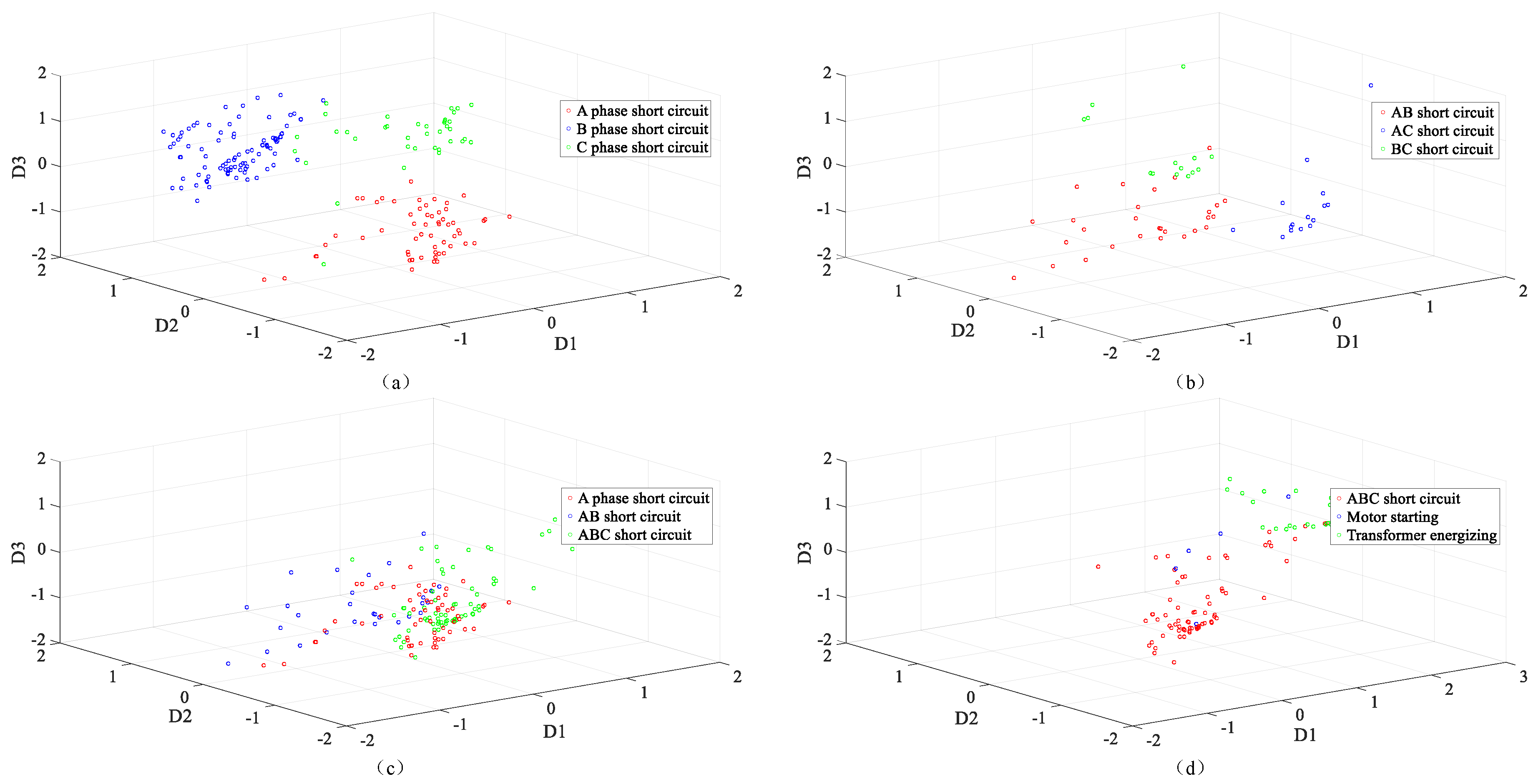
5.1. Separability Analysis of Voltage Sag Features

Separability connotes that, to achieve the classification objectives, the selection of features should follow certain principles. The features of different categories should be decentralized, and the features of the same categories should be congregated as far as possible. Features are the mathematical language that describe an event. Therefore, the feature data should contain as much information as possible about an event. Moreover, it is necessary to facilitate the establishment of a mathematical model. For appropriate voltage sag features, there are small spatial distances between features in the same categories and large spatial distances between features in different categories. In this paper, principal component analysis (PCA) was used to reduce the training samples from ten dimensions to three dimensions for display. Simultaneously, the average Euclidean distances of intraclass feature samples and interclass feature samples were calculated. Figure 9a–d shows the voltage sag feature distributions of A/B/C signal-phase short-circuit faults, AB/AC/BC two-phase short-circuit faults, A/AB/ABC-phase short-circuit faults, and three-phase short-circuit/motor starting/transformer energizing. These voltage sag features were extracted from sag data in the training set by PCA, and D1, D2, and D3 were three features of every sag sample.

Table 2. Euclidean distances of the features for different types of voltage sags.

Type	A	B	C	AB	AC	BC	ABC	Motor	Transformer
A	1.1191	2.0408	2.5008	2.3982	2.5290	2.7778	4.0343	2.0502	4.3169
B	2.0408	1.0767	2.0601	1.7949	2.0503	1,9248	3.4235	1.5793	3.2427
C	2.5008	2.0601	1.2672	2.3937	2.0669	2.1390	3.2183	1.9043	3.6703
AB	2.3982	1.7949	2.3937	1.4762	2.2754	2.3908	2.3836	2.2992	3.6218
AC	2.5290	2.0503	2.0669	2.2754	1.7498	2.3013	1.9764	2.4483	3.2359
BC	2.7778	1,9248	2.1390	2.3908	2.3013	1.4814	1.6136	2.1182	2.6700
ABC	4.0343	3.4235	3.2183	2.3836	1.9764	1.6136	1.3298	1.4589	2.2365
Motor	2.0502	1.5793	1.9043	2.2992	2.4483	2.1182	1.4589	1.9185	1.3246
Transformer	4.3169	3.2427	3.6703	3.6218	3.2359	2.6700	2.2365	1.3246	0.8121

shows the Euclidean distances of the features for different types of voltage sags.

The figures and table show that except for the voltage sag caused by motor starting, the intraclass feature samples had smaller Euclidean distances than did the interclass feature samples. The aggregation of identical category features and the decentralization of different category features were obvious. Therefore, the features proposed in this paper were suitable. For the voltage sag caused by motor starting, the intraclass features had larger Euclidean distances than did the transformer energizing, three-phase short-circuit, and B-phase short-circuit cases. Hence, the data of these types were mistakenly classified more easily in the recognition process of the DBN. The main reason was that the probability of occurrence of the motor starting sag was small, and real samples collected by an online monitoring system were inadequate. The feature distribution was more dispersive than that of other types of sag. Nevertheless, with continuous operation of the monitoring system and accumulation of historical data, this problem will be resolved, and the performance of these features will improve.

5.2. Training, Testing, and Comparison of the DBN network

In this paper, the deep learning model was built using the Deep Learn Toolbox master of MATLAB (R2016a, MathWorks, Natick, MA, USA). Because there were few input features, one hidden layer containing 100 neurons was established. There were 10 and 9 nodes in the first and last layer because there were 10 characteristic parameters and 9 types of voltage sag. The number of DBN training iterations was 50, the number of backpropagation neural network (BPNN) fine-tuning iterations was 1000, and the learning rate was 0.1. The input training samples of the DBN included 385 samples of 9 categories, and the sample format was $\left[Ve{l}_A,Ve{l}_B,Ve{l}_C,Re{s}_A,Re{s}_B,Re{s}_C,Re{c}_A,Re{c}_B,Re{c}_C,\mathrm{PVUR}\right]$. The output was the category labels. Figure 10 shows the global training error of the BPNN in fine-tuning reconstruction. The observed training error was stable and small after multiple iterations. Reconstructed error descended rapidly at the beginning of the iterations, which shows the satisfactory training effect. Then, 130 test samples were input into the DBN model, and the category label of each sample was obtained. The recognition results were shown in

Table 3. Recognition results of the DBN model.

		Actual Category
	Type	A (16)	B (34)	C (22)	AB (10)	AC (8)	BC (7)	ABC (23)	Motor (3)	Transformer (7)
Recognition Results	A	16
	B		34
	C			21	1
	AB				9			1
	AC				1	7
	BC						7
	ABC							22		1
	Motor								3
	Transformer									7

. There were four misclassified samples, and the overall recognition accuracy was 96.92%. Thus, the proposed model had high recognition accuracy in processing real voltage sag data.

To compare the recognition accuracy of the DBN established in this paper with other traditional pattern recognition models, the SVM model was built using the same training and test data. This model was established using LIBSVM 3.1 of MATLAB. The input training samples of SVM included 385 samples of nine categories, and the sample format was also $\left[Ve{l}_A,Ve{l}_B,Ve{l}_C,Re{s}_A,Re{s}_B,Re{s}_C,Re{c}_A,Re{c}_B,Re{c}_C,\mathrm{PVUR}\right]$. The parameters of the SVM were optimized by the cross-validation method, the penalty factor was c = 111.4305, and the kernel parameter was g = 0.0017. Then, 130 test samples were input into the SVM model. The results are shown in

Table 4. Comparison of the recognition accuracy results between the DBN and support vector machine (SVM).

Model	DBN	SVM
Accuracy	96.92%	93.08%

.

Based on the abovementioned test results, the following conclusions were drawn:

• The calculation method of the characteristic parameters was simple. Therefore, efficiency was high in processing online monitoring voltage sag data. However, the voltage sag parameters of the motor starting were too close to those of other types of sag in the feature space because the number of samples was too small and the spatial distribution was disperse. This problem will be solved with the accumulation of motor starting data by the online monitoring system.
• The recognition accuracy of the DBN model was satisfactory. Moreover, as an unsupervised modeling method, the model did not necessarily have to obtain the category labels of the training samples in advance. Only a small amount of typical data with labels was required for the reversed fine-tuning. For the online monitoring system, most of the data were unprocessed and had no category labels. Therefore, this model was suitable for online data processing.
• The DBN had a simpler parameter setting and better recognition accuracy than did the traditional SVM model. The SVM is suitable for data mining of small samples. However, the DBN is a better choice for the massive data collected by online monitoring systems. Moreover, the DBN has higher precision than SVM for voltage sag recognition, and the recognition accuracy will further increase with the expansion of training samples.

6. Conclusions

As an important part of power quality, the monitoring, judgement, and governance of voltage sag are consistently important issues that must be solved by power companies. A voltage sag monitoring system is the essential basis for solving these problems. However, with the expansion of monitoring scope and increases in sampling accuracy, the amount of voltage sag data will also dramatically increase over time. Processing such large amounts of data is difficult using the traditional manual methods. Therefore, valid information cannot be processed in time, and valuable information is discarded. The intelligent method proposed in this paper is effective in solving this problem, and the test results obtained based on actual data reflect the recognition accuracy of the approach.

• The proposed voltage sag parameters were well discriminated from one another. Parameters in the same category showed distinct agglomeration, and those in different categories showed distinct separability. This result demonstrated that the chosen parameters were reasonable.
• The recognition process, which was divided into offline training and online recognition, was appropriate. Historical data processing, feature extraction, and DBN model training were accomplished in offline processing. New sample data processing and recognition by the DBN model were performed online. The processing efficiency was high.

With the expansion of the training set and increase in training cycle number, the accuracy of the DBN model may be further improved. However, the recognition of voltage sag is only the first stage of voltage sag governance. Identifying the sag source location will be the focus of future research.

References

1. López, M.A.; de Vicuña, J.L.; Miret, J.; Castilla, M.; Guzmán, R. Control Strategy for Grid-Connected Three-Phase Inverters During Voltage Sags to Meet Grid Codes and to Maximize Power Delivery Capability. IEEE Trans. Power Electron. 2018, 33, 9360–9374. [Google Scholar] [CrossRef] [Green Version]
2. Xiao, X.Y.; Chen, Y.Z.; Wang, Y.; Ma, Y.Q. Multi-attribute analysis on voltage sag insurance mechanisms and their feasibility for sensitive customers. IET Gener. Transm. Distrib. 2018, 12, 3892–3899. [Google Scholar] [CrossRef]
3. Katic, V.A.; Stanisavljevic, A.M. Smart Detection of Voltage Dips Using Voltage Harmonics Footprint. IEEE Trans. Ind. Appl. 2018, 54, 5331–5342. [Google Scholar] [CrossRef]
4. Florencias-Oliveros, O.; González-de-la-Rosa, J.J.; Agüera-Pérez, A.; Palomares-Salas, J.C. Power quality event dynamics characterization via 2D trajectories using deviations of higher-order statistics. Measurement 2018, 125, 350–359. [Google Scholar] [CrossRef]
5. Liao, H.; Milanović, J.V.; Rodrigues, M.; Shenfield, A. Voltage Sag Estimation in Sparsely Monitored Power Systems Based on Deep Learning and System Area Mapping. IEEE Trans. Power Deliv. 2018, 33, 3162–3172. [Google Scholar] [CrossRef]
6. Beleiu, H.; Beleiu, I.; Pavel, S.; Darab, C. Management of Power Quality Issues from an Economic Point of View. Sustainability 2018, 10. [Google Scholar] [CrossRef]
7. Cisneros-Magañia, R.; Medina, A.; Anaya-Lara, O. Time-Domain Voltage Sag State Estimation Based on the Unscented Kalman Filter for Power Systems with Nonlinear Components. Energies 2018, 11. [Google Scholar] [CrossRef]
8. Xi, Y.; Li, Z.; Zeng, X.; Tang, X.; Liu, Q.; Xiao, H. Detection of power quality disturbances using an adaptive process noise covariance Kalman filter. Digit. Signal Process. 2018, 76, 34–49. [Google Scholar] [CrossRef]
9. Saini, M.K.; Beniwal, R.K. Detection and classification of power quality disturbances in wind-grid integrated system using fast time-time transform and small residual-extreme learning machine. Int. Trans. Electr. Energy Syst. 2018, 28. [Google Scholar] [CrossRef]
10. Jeevitha, S.R.S.; Mabel, M.C. Novel optimization parameters of power quality disturbances using novel bio-inspired algorithms: A comparative approach. Biomed. Signal Process. Control 2018, 42, 253–266. [Google Scholar] [CrossRef]
11. Branco, H.M.; Oleskovicz, M.; Coury, D.V.; Delbem, A.C. Multiobjective optimization for power quality monitoring allocation considering voltage sags in distribution systems. Int. J. Electr. Power Energy Syst. 2018, 97, 1–10. [Google Scholar] [CrossRef]
12. Bagheri, A.; Gu, I.; Bollen, M.; Balouji, E. A Robust Transform-Domain Deep Convolutional Network for Voltage Dip Classification. IEEE Trans. Power Deliv. 2018, 33, 2794–2802. [Google Scholar] [CrossRef]
13. Elbasuony, G.S.; Aleem, S.H.; Ibrahim, A.M.; Sharaf, A.M. A unified index for power quality evaluation in distributed generation systems. Energy 2018, 149, 607–622. [Google Scholar] [CrossRef]
14. Tang, Y.; Wei, R.; Chen, K.; Fang, Y. Voltage sag source identification based on the sign of internal resistance in a “Thevenin’s equivalent circuit”. Int. Trans. Electr. Energy Syst. 2017, 27. [Google Scholar] [CrossRef]
15. Chu, J.W.; Yuan, X.D.; Chen, B.; Wang, X.C.; Qiu, H.F.; Gu, W. A Method for Distribution Network Voltage Sag Source Identification Combining Wavelet Analysis and Modified DTW Distance. Power Syst. Technol. 2018, 42, 637–643. [Google Scholar] [CrossRef]
16. Thakur, P.; Singh, A.K. A novel method for joint characterization of unbalanced voltage sags and swells. Int. Trans. Electr. Energy Syst. 2017, 27. [Google Scholar] [CrossRef]
17. Barrera Nunez, V.; Velandia, R.; Hernandez, F.; Melendez, J.; Vargas, H. Relevant Attributes for Voltage Event Diagnosis in Power Distribution Networks. Rev. Iberoam. Autom. Inform. Ind. 2013, 10, 73–84. [Google Scholar] [CrossRef]
18. García-Sánchez, T.; Gómez-Lázaro, E.; Muljadi, E.; Kessler, M.; Muñoz-Benavente, I.; Molina-García, A. Identification of linearised RMS-voltage dip patterns based on clustering in renewable plants. IET Gener. Transm. Distrib. 2018, 12, 1256–1262. [Google Scholar] [CrossRef]
19. Gururajapathy, S.S.; Mokhlis, H.; Illias, H.A.; Awalin, L.J. Support vector classification and regression for fault location in distribution system using voltage sag profile. IEEJ Trans. Electr. Electron. Eng. 2017, 12, 519–526. [Google Scholar] [CrossRef]
20. Daud, K.; Abidin, A.F.; Ismail, A.P. Voltage Sags and Transient Detection and Classification Using Half/One-Cycle Windowing Techniques Based on Continuous S-Transform with Neural Network. In Proceedings of the 2nd International Conference on Applied Physics and Engineering (ICAPE), Penang, Malaysia, 2–3 November 2016. [Google Scholar] [CrossRef]
21. Kapoor, R.; Gupta, R.; Jha, S.; Kumar, R. Boosting performance of power quality event identification with KL Divergence measure and standard deviation. Measurement 2018, 126, 134–142. [Google Scholar] [CrossRef]
22. Zhao, R.; Yan, R.; Chen, Z.; Mao, K.; Wang, P.; Gao, R.X. Deep learning and its applications to machine health monitoring. Mech. Syst. Signal Process. 2019, 115, 213–237. [Google Scholar] [CrossRef]
23. Zhao, X.L.; Jia, M.P. A novel deep fuzzy clustering neural network model and its application in rolling bearing fault recognition. Meas. Sci. Technol. 2018, 29. [Google Scholar] [CrossRef]
24. Guo, Y.; Tan, Z.; Chen, H.; Li, G.; Wang, J.; Huang, R.; Liu, J.; Ahmad, T. Deep learning-based fault diagnosis of variable refrigerant flow air-conditioning system for building energy saving. Appl. Energy 2018, 225, 732–745. [Google Scholar] [CrossRef]
25. Tang, S.; Shen, C.; Wang, D.; Li, S.; Huang, W.; Zhu, Z. Adaptive deep feature learning network with Nesterov momentum and its application to rotating machinery fault diagnosis. Neurocomputing 2018, 305, 1–14. [Google Scholar] [CrossRef]
26. Yuan, N.; Yang, W.; Kang, B.; Xu, S.; Li, C. Signal fusion-based deep fast random forest method for machine health assessment. J. Manuf. Syst. 2018, 48, 1–8. [Google Scholar] [CrossRef]
27. Lin, J.; Su, L.; Yan, Y.; Sheng, G.; Xie, D.; Jiang, X. Prediction Method for Power Transformer Running State Based on LSTM_DBN Network. Energies 2018, 11. [Google Scholar] [CrossRef]
28. Garcia-Sanchez, T.; Gomez-Lazaro, E.; Muljadi, E.; Kessler, M.; Molina-Garcia, A. Statistical and Clustering Analysis for Disturbances: A Case Study of Voltage Dips in Wind Farms. IEEE Trans. Power Deliv. 2016, 31, 2530–2537. [Google Scholar] [CrossRef]
29. Hinton, G.E.; Osindero, S.; Teh, Y.W. A fast learning algorithm for deep belief nets. Neural Comput. 2006, 18. [Google Scholar] [CrossRef]
Figure 1. Typical waveforms of a single-phase short circuit. (a) Typical voltage root mean square (RMS) waveform of an A-phase short circuit; (b) typical voltage RMS waveform of a B-phase short circuit; (c) typical voltage RMS waveform of a C-phase short circuit.
Energies 12 00043 g001
Figure 2. Typical waveforms of a two-phase short circuit. (a) Typical voltage RMS waveform of A- and B-phase short circuits; (b )typical voltage RMS waveform of B- and C-phase short circuits; (c) typical voltage RMS waveform of A- and C-phase short circuits.
Energies 12 00043 g002
Figure 3. Typical voltage RMS waveform of a three-phase short circuit.
Energies 12 00043 g003
Figure 4. Typical voltage RMS waveform of a motor starting.
Energies 12 00043 g004
Figure 5. Typical voltage RMS waveform of a transformer energizing.
Energies 12 00043 g005
Figure 6. Voltage sag characteristic parameters.
Energies 12 00043 g006
Figure 7. Typical deep belief network (DBN) architecture.
Energies 12 00043 g007
Figure 8. Online voltage sag recognition process.
Energies 12 00043 g008
Figure 9. Voltage sag feature distribution in three dimensions. (a) Voltage sag feature distribution of A/B/C signal-phase short-circuit faults; (b) voltage sag feature distribution of AB/AC/BC two-phase short-circuit faults; (c) voltage sag feature distribution of A/AB/ABC-phase short-circuit faults; (d) voltage sag feature distribution of three-phase short circuit/motor starting/transformer energizing.
Energies 12 00043 g009
Figure 10. Global training error of the DBN in fine-tuning.
Energies 12 00043 g010