A Crane Overload Protection Controller for Blade Lifting Operation Based on Model Predictive Control

Abstract

Lifting is a frequently used offshore operation. In this paper, a nonlinear model predictive control (NMPC) scheme is proposed to overcome the sudden peak tension and snap loads in the lifting wires caused by lifting speed changes in a wind turbine blade lifting operation. The objectives are to improve installation efficiency and ensure operational safety. A simplified three-dimensional crane-wire-blade model is adopted to design the optimal control algorithm. A crane winch servo motor is controlled by the NMPC controller. The direct multiple shooting approach is applied to solve the nonlinear programming problem. High-fidelity simulations of the lifting operations are implemented based on a turbulent wind field with the MarIn and CaSADi toolkit in MATLAB. By well-tuned weighting matrices, the NMPC controller is capable of preventing snap loads and axial peak tension, while ensuring efficient lifting operation. The performance is verified through a sensitivity study, compared with a typical PD controller.

1. Introduction

The rapid development of offshore wind farms has been noticed with a trend of continued increasing in turbine size. The favor of larger offshore wind turbines (OWTs) results in decreasing costs of installation and grid connection per unit energy produced [1]. This comes with new challenges in offshore OWT installation. Single blade installation is a method of OWT blade installation, which allows for a broader range of installation vessels and lower crane capabilities. One blade is lifted in one lifting operation. Passive and active single blade installation methods have been studied [2,3,4,5,6,7].

Typically, the lifting operations are conducted according to pragmatic experiences and short-term weather forecast. The large peak wire rope tension in the initial stages of the lifting and lowering of a payload is risky for safety hazards. Extensive research has been conducted on effective crane and winch control. Various simplified models have been developed to model the crane and payload systems, e.g., Lagrangian models [8,9], Newton–Euler equations [10], and partial differential Equation [11]. Normally, the axial wire rope elongation is disregarded due to the its high stiffness. The ship-mounted crane systems have more complicated dynamic characteristics, with a higher number of degrees of freedom (DOFs) in the control system. A high-fidelity simulation-verification OWT blade installation model for the control purpose is developed in [4]. However, the model is unnecessarily complex for design of control laws. The ordinary studied payloads are lumped mass [12,13] and distributed mass [14]. Though wire rope elongation is always neglected in transportation mode, it is an important issue in e.g., heave compensation through a wave zone during moonpool operations [15,16,17,18,19].

Model predictive control (MPC) is a widely applied optimal control technology. The MPC controller provides real-time feedback by optimizing the future plant behavior in a finite horizon. Considerable effort has been devoted to improving its robustness and performance [20,21,22,23,24,25]. The performance of the nonlinear model predictive controller (NMPC) depends on the computation interval, initial guess, programming algorithms, etc. The stability can be ensured through a careful selection of designed parameters [26]. Direct methods transform a continuous system of infinite dimension into a discrete nonlinear programming system of finite dimension. The direct methods can be categorized into sequential and parallel-in-time approaches. Direct single shooting is a sequential approach, with a strong requirement to the initial guess, especially for highly nonlinear systems. However, the shortages of the parallel-in-time approach are the unnecessarily strong nonlinearity of the optimization problem and the poor convergence behaviors to the desired reference trajectory [27,28]. Optimization theories have been widely used in marine research [29,30,31]. To effectively solve the programming problem using embedded platforms, automatic code generation is a widely discussed issue. A number of user-friendly codes have been developed, where C++ codes for embedded systems can be generated automatically by several published quadratic programming solvers [32,33,34].

Though efforts have been made to improve the level of automation for blade mating operations [3,5,18,35,36], studies are lacking on constrained optimal blade lifting operations from the deck to improve safety and performance. An NMPC framework for lifting a lumped-mass payload was presented by the authors in [37]. In this paper, we extend the NMPC scheme for a winch servo to reduce the abrupt wire tension load increase and to avoid snap loads resulting from a suspended blade at the initial stages of lift-off (and also lowering) operation. This makes the transfer to the next phase, moving the blade towards the hub safer and more efficient. The main advantages of NMPC are that an optimal control action is achieved, where the performance and efficiency can be targeted by proper tuning of an objective function, while at the same time adhering to constraints that for other methods must be handled through implementation of logics. The lifted blade should reach the desired height in a specified speed abstaining from possible dangers. An optimal control problem is formulated for the lifting process of a blade, with implementation in a well-proven optimization solver. The performance and properties of the method, compared to a standard proportional-derivation (PD) crane lifting control law, are then demonstrated in a simulation study with a high-fidelity numerical model. In [37], only a simplified lifting system was considered, with a lumped-mass payload and known parameters, whereas wind-induced loads, motor dynamics, hook, and slings were neglected in the simulations. The extensions made in this paper therefore consist of deriving a reduced model for a more realistic blade payload in a lifting control design. Based on this, we design an NMPC controller to solve the formulated constrained optimal lifting problem in a turbulent wind field. Compared to a lumped-mass payload, a blade has more complex dynamics and aerodynamic characteristics. Simulations are finally conducted in turbulent wind fields with different mean wind speeds, as well as varying parametric uncertainties, and the simulation results are discussed.

The paper is structured as follows. In Section 2, the problem formulation is proposed with a description of the system and an illustrative example. A simplified model of the NMPC controller is introduced in Section 3. Basic concepts and theories concerning the direct multiple shooting approach are introduced in Section 4. Simulation results and comparative studies with a proportional-derivative (PD) controller are presented in Section 5. Finally, conclusions are drawn.

Notation: $\left|x\right|$ and ${\left|x\right|}_A$, respectively, denote the Euclidean vector norm and weighted Euclidean vector norm, i.e., ${\left|x\right|}^2=x^{\top }x$ and ${\left|x\right|}_A^2=x^{\top }Ax$ with $A=A^{\top }>0$. The vector inequality of $b\in {\mathbb{R}}^n$ is denoted by $\underline{b}⪯b⪯\overline{b}$, i.e., component-wise inequalities ${\underline{b}}_i\le b_i\le {\overline{b}}_i$ hold for $i=1,\cdots ,n$. Overlines and underlines, $\underline{b}$, $\overline{b}\in {\mathbb{R}}^n$, stand for vectors containing all the lower and upper limits of the elements in b, respectively. The saturation operator $\mathrm{sat}:\mathbb{R}\to \mathbb{R}$ is denoted by

$$\mathrm{sat}\left(a\right)=\left\{\begin{array}{cc}\overline{a}\hfill & \mathrm{if}a\ge \overline{a},\hfill \\ a\hfill & \mathrm{if}\underline{a}<a<\overline{a},\hfill \\ \underline{a}\hfill & \mathrm{if}a\le \underline{a}.\hfill \end{array}\right.$$

(1)

2. Problem Formulation

2.1. System Description

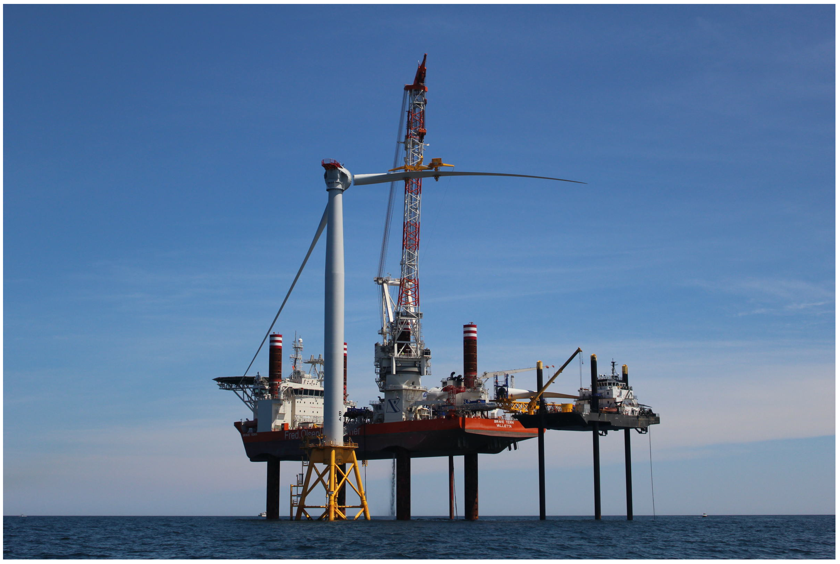
A jackup vessel is considered hereafter for the single blade installation operation. The legs have been lowered into the seafloor and the jack-up vessel has been lifted out of water, which provides a stable platform for lifting operations. The blade lifting operation is conducted by a rigidly fixed boom crane on the vessel. The blade is seized by a yoke through a lift wire and two slings; the configuration is shown in Figure 1 and Figure 2. A hook connects the lift wire and two slings. The yoke and crane boom are fastened by two horizontal tugger lines, constraining the blade motion within the horizontal plane due to the wind-induced loads. The lengths of the tugger lines are adjusted with the blade. Active tension force control on the tugger lines, such as [3], is not considered. The blade is first lifted up from the deck of the jackup or a barge, in which the lift wire gradually takes the gravity of the blade and the wind-induced dynamic loads. The blade is then lifted from a low position up to the hub height. During this phase, the main dynamic loads are the wind loads acting on the blades. If the lifting speed changes, the lift wire experiences the inertial loads on the blade. There are always gravity loads acting on the blade. When the blade is close to the hub height, one may reduce the lifting speed and adjust the position of the blade root for the final connection.

In this paper, we consider a scenario in which the blade starts in the air with a zero lifting speed. The supporting force from the deck is not considered. The lifting speed is increased to the target value and then reduced to zero when it reaches the specific hub height. The payload motion can be estimated by various methods, e.g., GPS and inertial measurement unit (IMU) sensor fusion algorithm and motion capture systems.

2.2. System Modeling

The blade installation simulation framework used is developed in MATLAB and Simulink [4], in which necessary modules for blade installation are included, e.g., wire rope, suspended blade, hook, winch, and wind turbulence. This approach has been applied to analyze and verify active single blade installation methods [3].

The hook and blade are modeled in 3DOF and 6DOF, respectively. Lift wires function as single-direction tensile springs that can only provide tension when the axial elongation is greater than zero. A turbulent wind field is generated by the Mann model in HAWC2. Because of the geometric complexity, the wind-induced loads are calculated according to the cross-flow principle. The total wind loads acting on the entire blade are the sum of the lift and drag forces measured at each airfoil segment.

An National Renewable Energy Laboratory (NREL) 5MW wind turbine blade is selected as the payload for a case study [39]. Due to physical limitations, the winch cannot reach a reference speed infinitely fast, nor exceed the designated safe speed. Hence, we assume the occurrence of saturation for both winch acceleration and winch speed. The main system parameters used are tabulated in

Table 1. Parameters of the single blade installation system.

Parameter	Symbol	Unit	Value
Mass of the blade	$m_t$	ton	$17.74$
Mass of the yoke	$m_t$	ton	20
Mass of the hook	$m_h$	ton	1
Initial length of the lift wire	${\overline{l}}_1\left(0\right)$	m	40
Length of the rope positioned in front of the pulley	$l_b$	m	60
Length of the slings	$l_s$	m	$9.17$
Elastic module	$EA$	N	$2.375\times {10}^9$
Modified coefficient	$\gamma$	-	0.5
Initial lifting speed	$l_2\left(0\right)$	$\frac{m}{s}$	0
Desired lifting speed	$v_{1d}$	$\frac{m}{s}$	$\pm 1.2$
Winch speed boundary	$[{\underline{v}}_1,{\overline{v}}_1]$	$\frac{m}{s}$	$[-1.2,1.2]$
Winch acceleration boundary	$[\underline{u},\overline{u}]$	$\frac{m}{s^2}$	$[-2,2]$

.

A local Earth-fixed, assumed inertial, reference frame is adopted with the x-, y-, and z-axes pointing in northern, eastern, and downward (NED) directions, respectively. Translational velocities measured along the axes are denoted $\dot{x}$, $\dot{y}$, and $\dot{z}$. The orientations about the fixed axes are given by roll, pitch, and yaw angles, denoted $\varphi$, $\theta$, and $\psi$, respectively.

2.3. Case Study

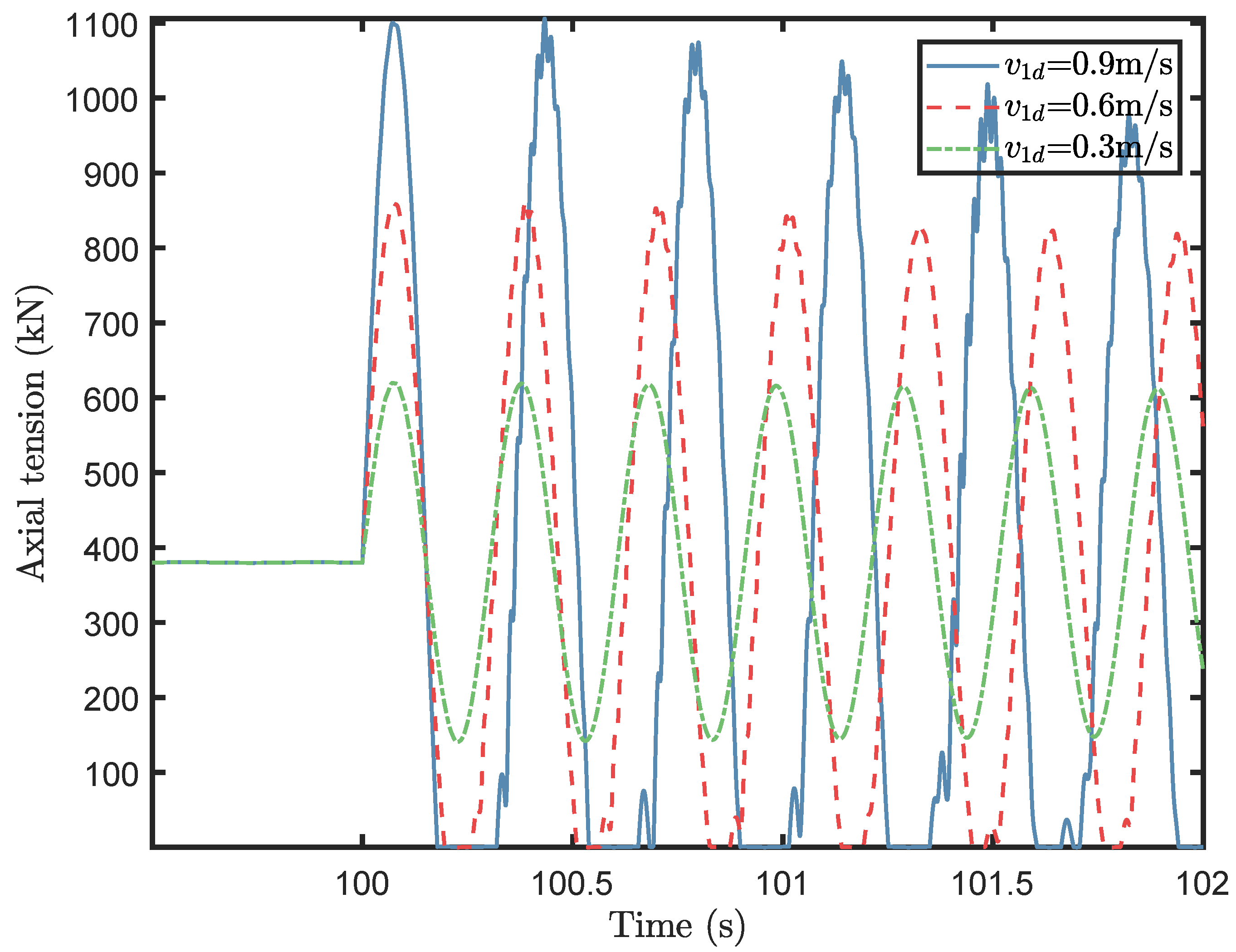
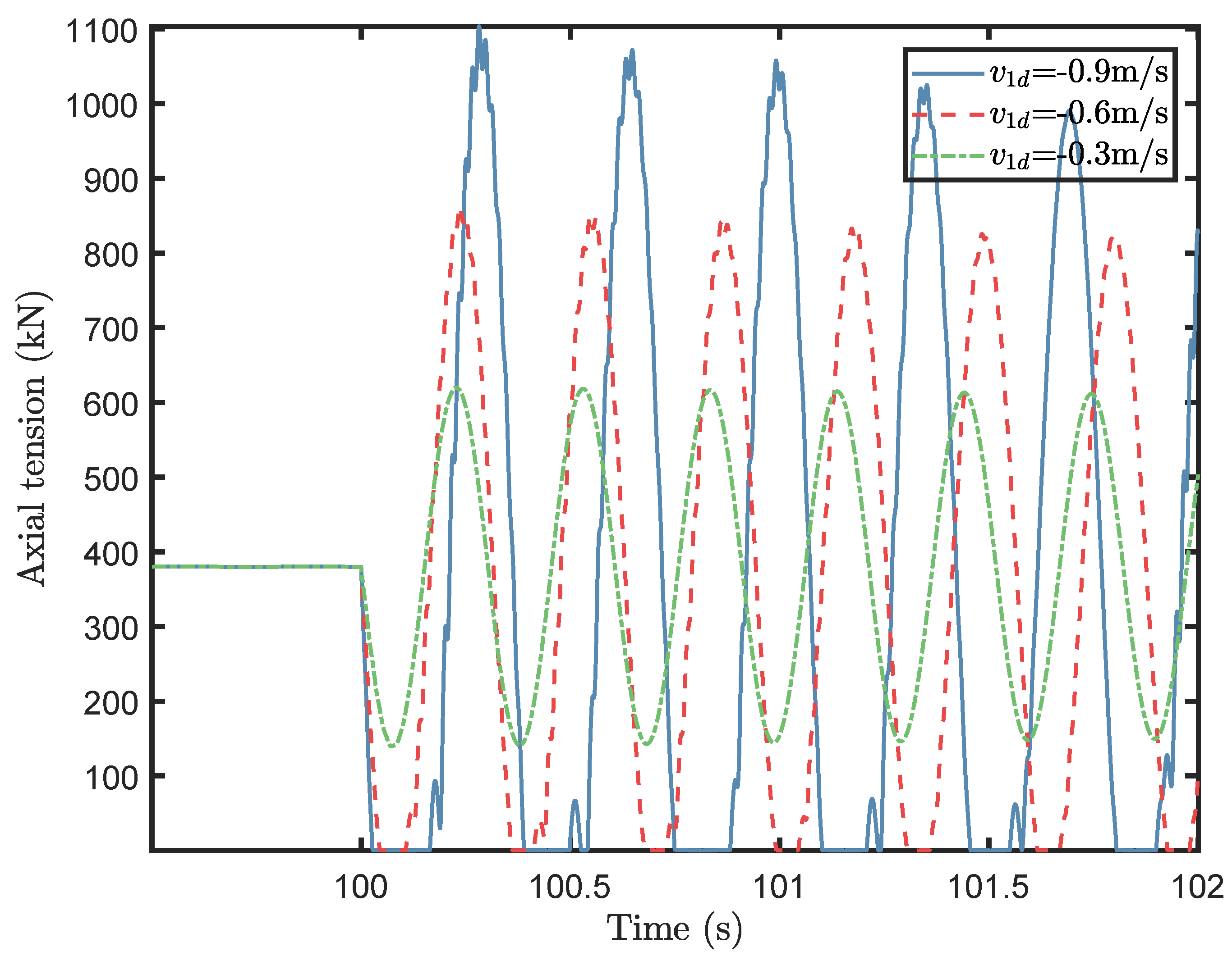
Since the blade is lifted off at a low level where the wind speed is low and the lift-off operation happens in a short duration of a few seconds, we consider a blade lift without aerodynamic loads. At the start of the simulation, the suspended blade is stabilized at an equilibrium point by the lift wire, slings, and tugger lines without oscillation in the lift wire. When a sudden lifting or lowering action is executed at 100 s, the lifting speed is changed to the constant desired speed $v_{1d}$ in a very short time. The wire tension history is shown in Figure 3 and Figure 4 for lifting and lowering, respectively.

In the figures, the only changing parameter is the setpoint lifting speed. It is observed that snap loads or sudden peak tensions are excited in the first 0.5 s, followed by the occurrence of damped oscillations due to the axial damping. The larger sudden tension occurs at the beginning of the lifting operation due to significant winch speed acceleration. The magnitude of the dynamic tension increases with the lifting speed.

In the tension history curves, there are some high-frequency peaks of minor amplitude, which are induced by the slings. The tension deviation caused by the blade’s motion in the horizontal plane is very small compared to the peak values. The amplitude of the oscillation decreases slowly.

Jerking occurs more easily at a higher lifting speed. A sudden tension maximum is dangerous. Snap loads, which occur when the axial tension decreases to below zero, are induced during this lifting operation. The maximum tension, on the other hand, may exceed the lift wire strength. Thus, the minimum value for the axial elongation of the wire should always be non-negative. The restoring force does not act on the payload due to the negative axial elongation when snap occurs. Furthermore, the magnitude of the blade motion is enlarged when snap loads occur, resulting in a potential impact damage between the blade and deck.

In practice, the lifting speed should be changed gradually from 0 to the setpoint speed to prevent the zero tension in the lift wire. In this paper, we show how constrained optimization conveniently can be designed to achieve this while simultaneously satisfying relevant constraints in the control system.

2.4. Problem Statement

The objective is to design a safe and efficient lifting scheme using constrained optimal control to achieve the necessary lifting performance. In more detail, there are seven optimal targets:

(a)

Reach the desired setpoint lifting speed $v_{1d}$ from zero speed in the shortest time possible within the constraints,

(b)

Protect overload tension and reduce dynamic tension by controlling the winch speed,

(c)

Prevent winch servo motor burnout by limiting the winch acceleration,

(d)

Prevent negative elongation and snap loads,

(e)

Reduce the wire rope wear,

(f)

Limit the maximum speed of the servo motor,

(g)

Reach the desired wire rope length.

The tugger lines are assumed to be released with the lifting operation. Therefore, tugger lines do not provide restoring forces unless wind-induced blade displacement is higher than expected. We assume that the blade orientation variance caused by the lifting operation and the wind-induced load is insignificant, and the lifting or lowering operation is so short that wind-induced motion is not affected.

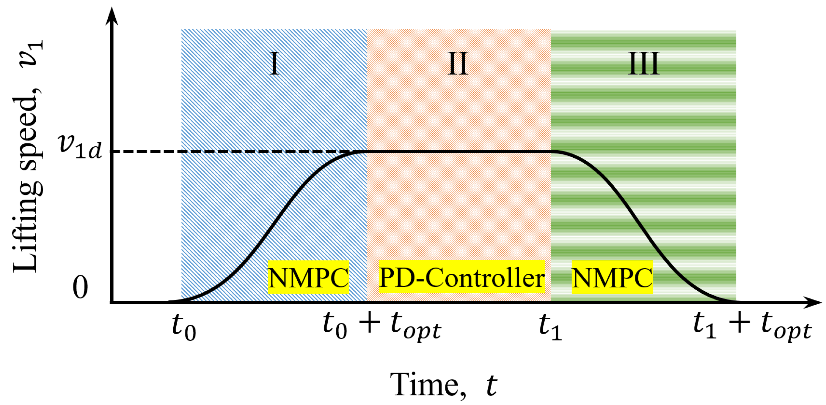
A lifting process is divided into three phases: the startup region, the steady region, and the slowdown region; see Figure 5. The control objective of each region is tabulated in

Table 2. Objectives for Regions I and III.

Objective No.	Region I	Region III
(a)	✔	✔
(b)	✔	✔
(d)	✔	✔
(d)	✔	✔
(e)	✔	✔
(f)	✔	✔
(g)		✔

. Region I denotes the startup stage, wherein the payload speeds up to the desired lifting speed $v_{1d}$ from initial winch speed $v_1\left(0\right)=0$. Sudden overloads or snap loads mainly occur at the beginning of Region I. In Region II, spanning from the end of the startup stage to the outset of the slowdown stage, a steady motion is performed. The purpose of this stage is to ensure the desired lifting speed, i.e., $v_1\left(t\right)=v_{1d}$. The controller should be deactivated during this stage due to the low dynamic tension. Instead, a simple proportional controller is used in this phase for its simplicity. Region III is the slowdown stage, where the controller is again activated. The lifting speed should be reduced to zero. Dynamic tension mainly occurs in the initial period. In addition to all requirements for Region I, the desired wire rope length should be achieved. The controller is switched off at the end of Region III.

3. Reduced Model for Control Design

A reduced model is adopted for the optimization problem in a three-dimensional north–east–down (NED) coordinate system [40]. The crane is assumed to be rigidly fixed on the vessel. The masses of the hook, yoke, and blade are $m_h$, $m_y$, and $m_b$, respectively. We assume that the overall payload mass $m_t$ is concentrated at the blade center of gravity (COG), where $m_t=m_h+m_y+m_b$. Furthermore, the lift wire and slings are considered as one unit without the consideration of the lift wire control; it provides a restoring force on the moving blade. We assume that the ropes are replaced by a lightweight rope, i.e., its mass is assumed to be zero. The blade COG is suspended by the rope, which is connected to the winch through a pulley fixed at the crane tip. Hence, a tensile spring is employed to model the wire rope. The unstretched length of the spring ${\overline{l}}_1$ denotes the distance between the pulley and blade COG. Tugger lines are released at a speed such that only vertical lifting is allowed. Because the lifting operation is executed over a short period, the horizontal wind-induced load is assumed to be restrained by tugger lines and can be disregarded. A 3DOF lifting model, with an elastic wire rope and a controllable winch, is deduced based on the Newton–Euler method in the NED coordinate system. Four vectors are defined correspondingly:

$$\begin{array}{c}\mathrm{the}\mathrm{position}\mathrm{of}\mathrm{the}\mathrm{blade}\mathrm{COG}:r_t={[x_t,y_t,z_t]}^{\top },\hfill \\ \mathrm{the}\mathrm{position}\mathrm{of}\mathrm{the}\mathrm{pulley}:r_p={[x_p,y_p,z_p]}^{\top },\hfill \\ \mathrm{the}\mathrm{translational}\mathrm{velocity}\mathrm{of}\mathrm{the}\mathrm{blade}\mathrm{COG}:u_t={[{\dot{x}}_t,{\dot{y}}_t,{\dot{z}}_t]}^{\top },\hfill \\ \mathrm{the}\mathrm{velocity}\mathrm{of}\mathrm{the}\mathrm{pulley}:u_p={[{\dot{x}}_p,{\dot{y}}_p,{\dot{z}}_p]}^{\top }.\hfill \end{array}$$

The total force acting on the payload is given by

$$M_t{\dot{u}}_t=G+{\tau }_{tr}+{\tau }_{td},$$

(2)

where the mass matrix is written as $M_t=\mathrm{diag}(m_t,m_t,m_t)$, G, ${\tau }_{tr}$, ${\tau }_{td}$ are the gravity, restoring force, and damping force, respectively. If the lifting speed changes quickly, the main reason for the large dynamic tension is from the lifting wire. Then, the blade wind loads could be considered as quasi-static loads. Hence, the controller is not developed to compensate the dynamic tension due to the disturbance in wind.

3.1. Restoring Force

Additional two vectors are defined to shorten the equations. The relative position vector from the pulley to payload ${\Delta }_1$ and its time derivative ${\Delta }_2$ are respectively defined as

$$\begin{array}{c}{\Delta }_1:=r_t-r_p,\end{array}$$

(3a)

$$\begin{array}{c}{\Delta }_2:=u_t-u_p.\end{array}$$

(3b)

The restoring force of the lift wire ${\tau }_{tr}$ reacts with positive wire rope axial elongation, i.e.,

$${\tau }_{tr}=-\kappa \left(\delta \right)k_r\delta \frac{{\Delta }_1}{\left|{\Delta }_1\right|},\kappa \left(\delta \right)=\left\{\begin{array}{cc}1,\hfill & \delta \ge 0,\hfill \\ 0,\hfill & \mathrm{otherwise},\hfill \end{array}\right.$$

(4)

where $\kappa$ denotes the restoring action coefficient, $\delta =\left|{\Delta }_1\right|-{\overline{l}}_1$ is the elastic elongation, and $k_r$ is the stiffness. Determined by the material, diameter, and strand construction, the generalized stiffness of the rope is modeled as

$$k_r=\gamma \frac{E{A}_r}{l_1},$$

(5)

where $\gamma$ is the modified coefficient of a stranded wire, E stands for the Young’s modulus, $A_r$ denotes the cross-sectional area of the rope, and $l_1={\overline{l}}_1+l_b$, where we assume that the length of rope between the winch and pulley $l_b$ is constant.

3.2. Damping

The wire rope has a small damping ratio, generally selected as $0.1$–$0.5\%$ of the critical damping value [41]. Hence, the damping force ${\tau }_{td}$ is given by

$${\tau }_{td}=-d_l\dot{\delta }\frac{{\Delta }_1}{\left|{\Delta }_1\right|}=-\frac{d_l}{\left|{\Delta }_1\right|}(\frac{{\Delta }_1^{\top }{\Delta }_2}{\left|{\Delta }_1\right|}-v_1){\Delta }_1,$$

(6)

where $v_1$: $={\dot{l}}_1$ denotes the wire length changing rate, $d_l$ is the damping coefficient, and the elongation changing rate $\dot{\delta }$ is given by

$$\begin{array}{c}\hfill \dot{\delta }=\frac{{\Delta }_1^{\top }}{\left|{\Delta }_1\right|}{\Delta }_2-v_1.\end{array}$$

(7)

3.3. Winch Servo Motor

A variable-speed DC motor with motion feedback control is used as the winch servo motor to follow the specific motion trajectory. The field voltage is employed as an input for the DC motor. The produced magnetic torque $T_m$ is proportional to the armature current $i_f$, given by

$$T_m=k_m{i}_f=T_l+T_d,$$

(8)

where $k_m$ is the motor constant, $T_l$ is the load torque, and $T_d$ is the disturbance torque. The transfer function between $i_f$ and the field voltage $V_f$ is given by

$$\frac{i_f}{V_f}\left(s\right)=\frac{1}{R_f+L_{f}s},$$

(9)

where $R_f$ and $L_f$ are the armature resistance and inductance. The transfer function between the winch servo motor acceleration, $u={\dot{v}}_1$, and $T_l$ is given by

$$\frac{u}{T_l}\left(s\right)=\frac{s/r_m}{J_{m}s+B_m},$$

(10)

where $r_m$ is the radius of the winch, $J_m$ is the moment of inertial, and $B_m$ denotes the viscous friction coefficient. The low-level servo motor speed and torque control is not discussed in this paper. We assume that the field-current-controlled motor can effectively track the signal u generated from the proposed controller.

3.4. Model Summary

Under the aforementioned assumptions, disregarding wind-induced loads and substituting Equations (4) and (6) into Newton’s second law (2), the simplified control design model for the considered blade lifting operation is produced,

$$\begin{array}{cc}\hfill {\dot{r}}_t& =u_t,\hfill \end{array}$$

(11a)

$$\begin{array}{cc}\hfill M_t{\dot{u}}_t& =-A(r_t,r_p,l_1,v_1){\Delta }_1+G,\hfill \end{array}$$

(11b)

$$\begin{array}{cc}\hfill {\dot{l}}_1& =v_1,\hfill \end{array}$$

(11c)

$$\begin{array}{cc}\hfill {\dot{v}}_1& =u,\hfill \end{array}$$

(11d)

where $A(r_t,r_p,l_1,v_1)=a_t{I}_{3\times 3}$, with $a_t=\gamma EA\frac{\left|{\Delta }_1\right|-{\overline{l}}_1}{l_1\left|{\Delta }_1\right|}+\frac{d_l}{\left|{\Delta }_1\right|}(\frac{{\Delta }_1^{\top }{\Delta }_2}{\left|{\Delta }_1\right|}-v_1)$, and $G={[0,0,m_{t}g]}^{\top }$ is gravity. The nonlinearity of the differential Equation (11) mainly derives from the function $a_t$.

4. Design of the Optimal Control

NMPC is adopted to solve the proposed constrained optimization problem. Numerical nonlinear optimization involves finding suitable inputs for a complex nonlinear system that minimizes a specified performance objective within system constraints. The direct multiple shooting approach is adopted hereafter for discretization, and the ODE (11) is used for prediction.

4.1. Direct Multiple Shooting Method

A continuous optimal control problem is transformed into a nonlinear programming (NLP) problem through a direct multiple shooting approach. According to the discretization of the state variables and control inputs for finite dimensional parameterization of the path constraints, shooting nodes and piecewise functions are adopted to approximate the variables. Then, a quasi-Newton method is employed to solve it.

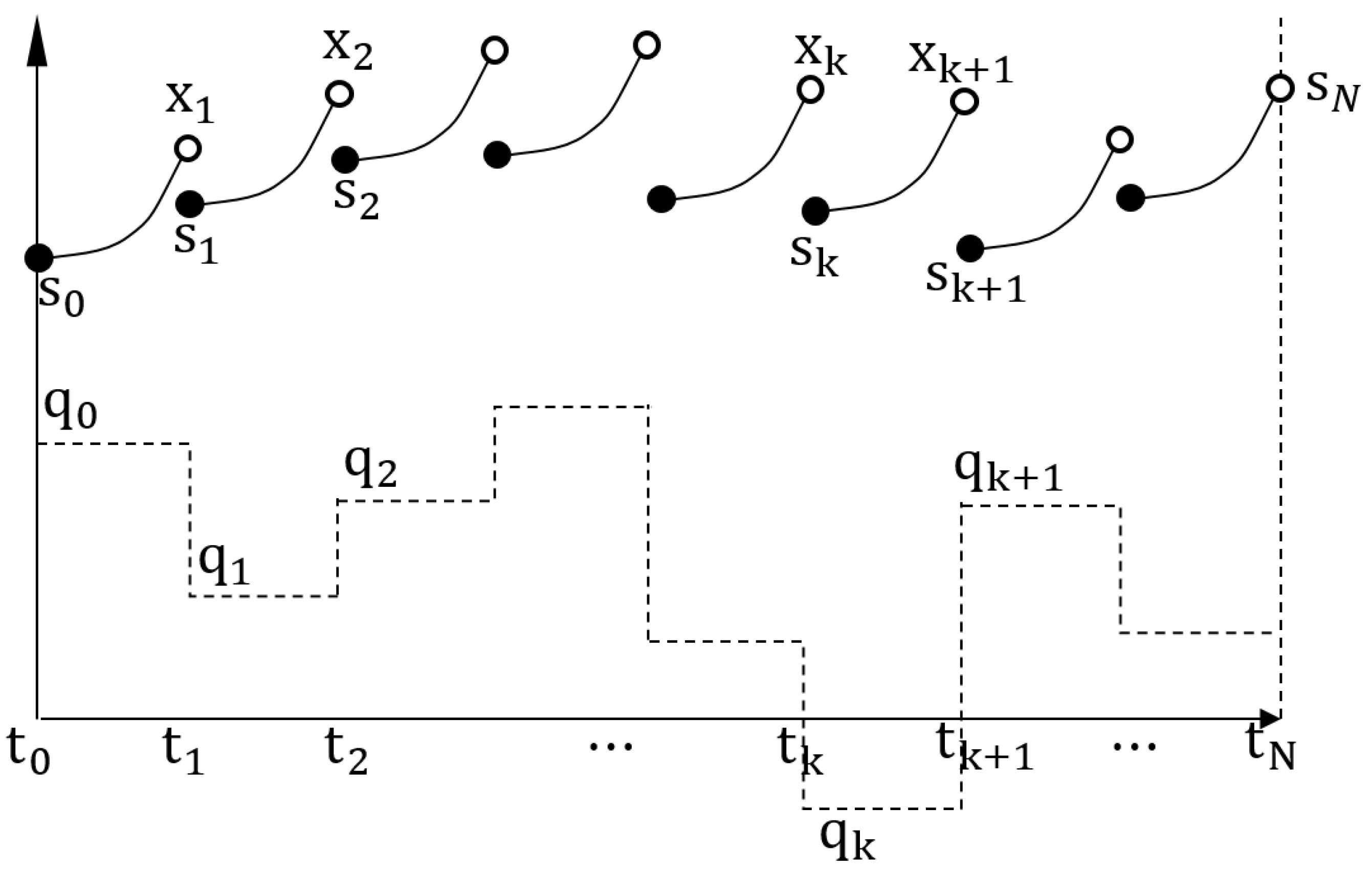
A time grid $t_0<t_1<\cdots <t_N$ is generated over a time horizon $[t_0,t_0+T]$ by dividing the period into N subintervals with a constant time step equal to the sampling time, i.e., $\delta t=T/N$. To simplify the expression, $x\left(t_k\right)$ is denoted by $x_k$, where $t_k=t_0+k\delta t$. For a subinterval $[t_k,t_{k+1}]$, the state numerically updates with the explicit integrator F and approximates the solution mapping, i.e., $x_{k+1}=F(x_k,u_k)$. Two additional variables, $s_i$ and $q_i$, are introduced as discrete representations of x and u, respectively, i.e., $s_{k+1}=F_k(s_k,q_k)$. Zero-order hold is used as the feedback signal input from a finite-dimensional NLP problem during subinterval $[t_k,t_{k+1}]$. The notations of the above processes are presented in Figure 6.

A dynamic optimization problem with constraints can be solved using a multiple shooting approach, which is formulated as

$$\begin{array}{c}\underset{S,Q}{min}\frac{1}{2}\sum _{k=0}^{N-1}{l}_k(s_k,q_k)+E_N\left(s_N\right),\hfill \end{array}$$

(12a)

$$\begin{array}{cc}\hfill \mathrm{s}.\mathrm{t}.& x_0-s_0=0,\hfill \end{array}$$

(12b)

$$\begin{array}{cc}F(t_{k+1};t_k,s_k,q_k)-s_{k+1}=0,\hfill & \hfill k=0,\cdots ,N-1,\end{array}$$

(12c)

$$\begin{array}{cc}h(s_k,q_k)⪯0,\hfill & \hfill k=0,\cdots ,N,\end{array}$$

(12d)

$$\begin{array}{c}r\left(s_N\right)⪯0,\hfill \end{array}$$

(12e)

where $S=[s_1,\cdots ,s_N]$ denotes the state trajectory containing all the the state vector at the kth time interval $x_k$, $Q=[q_1,\cdots ,q_{N-1}]$ refers to the control trajectory, equations (12b–12e) denote the initial value, continuity condition, path constraints, and terminal constraints, respectively. The objective function, which consists of an integral cost contribution (or Lagrange term) $l_k$ and an end time cost contribution (or Mayer term) $E_N$, can be chosen as, e.g.,

$$\begin{array}{cc}\hfill l_k(s_k,q_k)& ={|s_k-x_k^{ref}|}_{\mathcal{Q}}^2+{|q_k-u_k^{ref}|}_{\mathcal{R}}^2,\hfill \\ \hfill E_N\left(s_N\right)& ={|s_N-x_N^{ref}|}_{\mathcal{P}}^2,\hfill \end{array}$$

where $\mathcal{Q}$, $\mathcal{R}$, and $\mathcal{P}$ denote positive-definite diagonal weighting matrices.

An example of the path is given by

$$\begin{array}{ccc}\hfill \underline{u}& ⪯u_k⪯\overline{u},\hfill & \hfill k=0,\cdots ,N-1,\\ \hfill \underline{s}& ⪯s_k⪯\overline{s},\hfill & \hfill k=0,\cdots ,N-1,\end{array}$$

where $\underline{s}$, $\overline{s}$, $\underline{u}$, and $\overline{u}$ are the lower and upper limits for state s and input u. The limits can be chosen according to the critical operational conditions and physical actuator constraints. The desired trajectory for $s_k$ and $q_k$ are denoted by $x_k^{ref}$ and $u_k^{ref}$. Several established methods can be used to solve the NLP problem, e.g., interior point methods [42,43,44] and genetic algorithms [45,46].

4.2. NMPC Design

For the blade lifting problem, the NLP problems in Regions I and III are summarized in

Table 3. Summary of the control algorithm for different regions.

Region	Control Law
I	$$\underset{S,Q}{min}\sum _{k=0}^N[k_{\delta }(\frac{d}{dt}|{\Delta }_1|-v_1{)}^2+k_d{(v_1-v_{1d})}^2]+\sum _{k=0}^{N-1}{k}_u{u}^2,$$ (13a)
	$$\mathrm{s}.\mathrm{t}.\underline{u}\le u\le \overline{u},k=0,\cdots ,N-1,$$ (13b)
	$$|{\Delta }_1|-{\overline{l}}_1\ge 0,k=0,\cdots ,N,$$ (13c)
	$${\dot{|\Delta |}}_1-v_{1d}=0,k=N;$$ (13d)
II	$$u=-k_p(v_1-v_{1d});$$ (14)
III	$$\underset{S,Q}{min}\sum _{k=0}^N[k_{\delta }(\frac{d}{dt}\left|{\Delta }_1\right|-v_1{)}^2+k_d{(v_1-v_{1d})}^2+k_l{({\overline{l}}_1-{\overline{l}}_{1d})}^2]+\sum _{k=0}^{N-1}{k}_u{u}^2,$$ (15a)
	$$\mathrm{s}.\mathrm{t}.\underline{u}\le u\le \overline{u},k=0,\cdots ,N-1,$$ (15b)
	$$|{\Delta }_1|-{\overline{l}}_1\ge 0,k=0,\cdots ,N,$$ (15c)
	$${\dot{|\Delta |}}_1-v_{1d}=0,k=N,$$ (15d)
	$${\overline{l}}_1-{\overline{l}}_{1d}=0,k=N;$$ (15e)

.

In Table 3, $k_p>0$ is the gain of the P controller, and $k_u$, $k_{\delta }$, and $k_d$ are the weights for different components in the cost function. Quadratic objective functions are adopted. The physical meaning of different equations are explained as follows: in equations (13a) and (15a), ${\left(\frac{d}{dt}\left|{\Delta }_1\right|-v_1\right)}^2$, ${(v_1-v_{1d})}^2$, ${({\overline{l}}_1-{\overline{l}}_{1d})}^2$, and $u^2$ penalize the relative speed between the payload and winch, the deviation between the real-time winch speed and the desired final winch speed, the difference between the real-time lift wire length and the desired final length, and the winch input, respectively. The corresponding targets of these terms in Section 2.4 are (b,e), (a,f), (g), and (c), respectively. The objectives of the inequality constraints (13b) and (13c) are (c) by limiting the control input and (d) by ensuring that elongation is always non-negative. The selection of the boundary values $\underline{u}$ and $\overline{u}$ depends on characteristics and configuration of the winch. The equality constraints (13d) and (15e) ensure that the lifting speed and lift wire length reach their specified values at the final time.

For the proposed model in (11), there are eight states and one control input. The initial prediction is significant for the computational efficiency and stability. Figure 7 and Figure 8 show an example of the weight selection with respect to the time interval $t_k$, $k=0,\cdots ,N-1$. Sudden tension peaks occur at the beginning of the start up and slowdown phases. Hence, high weights are selected for $k_{\delta }$ at the beginning period to prevent significant sudden overload, and similarly high weights are needed for $k_d$ at the end of the period to achieve desired lifting speed.

4.3. Stability Considerations

Define new states as $x_1=\left|{\Delta }_1\right|-{\overline{l}}_1-\frac{mg{l}_1}{\gamma EA}$, $x_2={\dot{x}}_1=\frac{d}{dt}\left|{\Delta }_1\right|-(1+\frac{mg}{\gamma EA})v_1$ with $\frac{d}{dt}\left|{\Delta }_1\right|=\frac{{\Delta }_1^{\top }{\Delta }_2}{\left|{\Delta }_1\right|}$, $x_3=l_1-l_{1d}$, and $x_4={\dot{x}}_3=v_1-v_{1d}$. The dynamics are given by

$$\begin{array}{cc}\hfill {\dot{x}}_1=& x_2,\hfill \end{array}$$

(16a)

$$\begin{array}{cc}\hfill {\dot{x}}_2=& -\frac{1}{{\left|{\Delta }_1\right|}^3}{\left({\Delta }_1^{\top }{\Delta }_2\right)}^2+\frac{1}{\left|{\Delta }_1\right|}{\Delta }_2^{\top }{\Delta }_2+\frac{1}{\left|{\Delta }_1\right|}{\Delta }_1^{\top }{\dot{\Delta }}_2-(1+\frac{mg}{\gamma EA})u,\hfill \end{array}$$

(16b)

$$\begin{array}{cc}\hfill {\dot{x}}_3=& x_4,\hfill \end{array}$$

(16c)

$$\begin{array}{cc}\hfill {\dot{x}}_4=& u-{\dot{v}}_{1d}\left(t\right).\hfill \end{array}$$

(16d)

The vector form is

$$\dot{x}=f(t,x,u),x\left(t_0\right)=x_0,t\ge t_0\ge 0,$$

(17)

where $x={[x_1,x_2,x_3,x_4]}^{\top }$ and u is constrained, i.e., $u\in U$.

Function f is twice continuously differentiable. For $x=0$, we have that $\left|{\Delta }_1\right|={\overline{l}}_1+\frac{mg{l}_1}{\gamma EA}$ is a constant, $l_1=l_{1d}$, and $v_1=v_{1d}$. Hence, $\frac{d}{dt}\left|{\Delta }_1\right|=0$, ${\Delta }_1^{\top }{\Delta }_2=0$, ${\left|{\Delta }_2\right|}^2=0$. When the crane pulley is fixed, ${\dot{\Delta }}_2={\dot{u}}_t=0$. In addition, if $u=0$, we get $f(t,0,0)=0$ for all $t\ge t_0$. From (13b) and (15b), $u=0$ is included in U, and U is a compact and convex set. Hence, system (16) has a unique solution for any initial condition $x_0$ and piecewise continuous input $u\left(t\right)$, $t\ge 0$. Furthermore, the Jacobian linearization of the nonlinear system (16) is stabilizable. In our case, starting in Region I at zero velocity and Region III from a constant desired speed, a feasible solution is a matter of accelerating slowly enough. Hence, feasibility solutions always exist so that there exists at least one input profile Q for which all the constraints are satisfied. Therefore, according to the Theorem 1 in [47], the closed-loop system (16) with optimal control problem (13) and (15) is asymptotically stable, if a sufficiently small sampling time $\delta t$ is adopted and there exist no disturbances.

4.4. Overview of the Control System

A block diagram of the control scheme is presented in Figure 9. As several controllers are proposed in Table 3, a switching logic outputs a signal $\sigma$ to determine the working controller used for a specific period. The switching rule is given in Algorithm 1, where $\sigma =0$ denotes that all controllers are switched off and $\sigma \in \{1,2,3\}$ is the index of the corresponding controller; $\mu \in (0,1)$ is a coefficient setting the boundary of Controller I. The feedback to the controller I is the position and velocity of the payload, length of lift wire, and winch servo motor speed. The feedback to the PD controller is the length of lift wire and winch servo motor speed.

In addition, an observer is needed to filter the sensor noise and estimate unmeasured states in practical applications [48]. Observer design is not the emphasis of this paper and therefore not considered.

Algorithm 1 Switching rule.

Data: ($l_1,v_1,\mu ,l_{1d},v_{1d},l_s$)

Initialize: $\sigma =0$

if operation starts

if ($\sigma =0$ or 1) and $v_1<\mu v_{1d}$

$\sigma =1$

elseif ($\sigma =1$ or 2) and $v_1\ge \mu v_{1d}$

$\sigma =2$

elseif ($\sigma =2$ or 3) and $0\le |l_1-l_{1d}|\le l_s$

$\sigma =3$

end

else

$\sigma =0$

end

Return: $\sigma$

5. Simulations and Results

5.1. Simulation Overview

The simulations are conducted in MATLAB. The structural parameters used are tabulated in Table 1. The limits of the winch loads are considered to be expressed by the maximum acceleration. The wind field with turbulence starts acting on the blade with a ramp over the first five seconds. Class C turbulent winds with corresponding turbulence intensity ($TI$) are adopted in the simulations [49]. CaSADi and MarIn toolboxes are used to solve the NLP problems. The ipopt solver is adopted.

The simulation scenario involves lowering a suspended NREL 5 MW wind turbine blade 10 m. The initial wire length is ${\overline{l}}_1=40$ m, the final desired length is ${\overline{l}}_1=50$ m, and the final desired lifting speed is $v_{1d}=1.2$ m/s. The control horizon is $t_{opt}=4$ s with 40 subintervals. The following parameters are used for the different regions:

(a)

Region I: Start a lifting with an initial wire length and initial speed, and reach a desired speed in $t_{opt}$:

• ${\overline{l}}_1\left(t_0\right)=40$ m,
• $v_1\left(t_0\right)=0$ m/s,
• $v_1(t_0+t_{opt})=v_{1d}=1.2$ m/s.

(b)

Region II: Stabilize the lifting speed to the desired value:

• $v_1\left(t\right)=v_{1d}=1.2$ m/s.

(c)

Region III: Stop the lifting operation with the following initial speed, and reach the desired lift wire length in $t_{opt}$:

• $v_1\left(t_1\right)=1.2$ m/s,
• $v_1(t_1+t_{opt})=0$ m/s,
• ${\overline{l}}_1(t_1+t_{opt})=50$ m.

Tugger lines are released with a speed of $v_{tug}$, i.e.,

$$v_{tug,i}=\frac{z_t-z_{tug,i}}{l_{tug,i}}{v}_1,$$

(18)

where subscript i is the index of the tugger line, $z_{tug}$ is the vertical position of the tugger line connection point to the crane boom, and $l_{tug}$ is the length of the tugger line.

5.2. Basic PD Controller

To compare the NMPC controller performance, PD controllers are used. These open-loop controllers accelerate the winch servo motor to the desired speed. Due to physical limitations of the actuator (winch servo motor), saturation modules are applied to bound the lifting acceleration and velocity. A lowpass filter is used as a reference model. In summary, the combination of the lowpass filter and PD controller is given by

$$\begin{array}{cc}\hfill {\dot{l}}_d& =-{\omega }_{v1}(l_d-l_{ref}),\hfill \end{array}$$

(19a)

$$\begin{array}{cc}\hfill {\dot{\overline{l}}}_1& =\mathrm{sat}\left(v_1\right),\hfill \end{array}$$

(19b)

$$\begin{array}{cc}\hfill u& =\left\{\begin{array}{cc}\mathrm{sat}\left(-{\omega }_{v1}^2({\overline{l}}_1-l_d)-2{\zeta }_{v1}{\omega }_{v1}{v}_1\right),\hfill & \mathrm{Reg}.\mathrm{I},\mathrm{III},\hfill \\ \mathrm{sat}\left(-k_{v1}(v_1-v_{1d})\right),\hfill & \mathrm{Reg}.\mathrm{II},\hfill \end{array}\right.\hfill \end{array}$$

(19c)

where $l_{ref}$ and $l_d$ denote the final reference and desired trajectory for the lift wire length, ${\zeta }_{v1}$ is the relative damping ratio, and ${\omega }_{v1}$ is the natural frequency. Select ${\zeta }_{v1}=1$ to ensure critical damping. Different ${\omega }_{v1}$ values are assigned to different regions. In Region II, ${\omega }_{v1}$ can be smaller than ${\omega }_{v1}$ in Regions I and III. In the simulation, ${\omega }_{v1}=0.57$ in Region I and III and $k_p=0.5$ in Region II.

5.3. Comparative Simulation Results

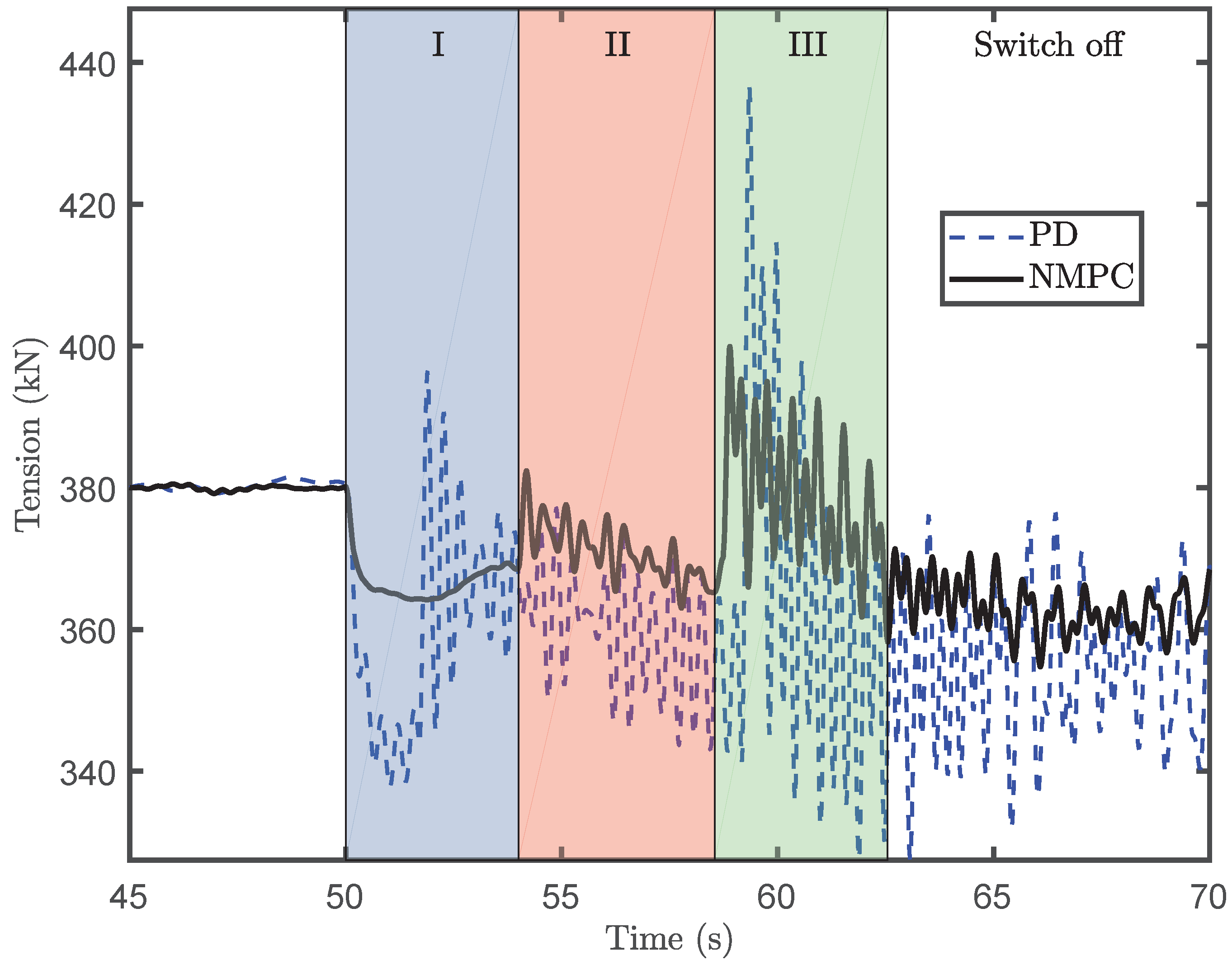
By well-tuned weighting matrices, the simulation results are illustrated in Figure 10, Figure 11, Figure 12, Figure 13 and Figure 14. In the simulations, $\gamma =0.5$ is used in the NMPC controller. Each bar presents the mean value of five simulations with different turbulence seeds.

Note that this is not an accurate value because the overall stiffness is influenced by the slings. The simulations feature a difficult scenario with a short Region II. Typically, the Region II operation can be much longer than five seconds, so that the transient effect in the lifting wire tension may die out. Hence, the maximum dynamic tension in the results simulated here may be higher than those with a longer Region II. The controller is switched off at the end of Region III.

Both the PD controller and NMPC controller are successful at lifting the payload to the desired position at the required speed. However, much less dynamic tension is generated by the NMPC controller than by the PD controller. The PD controller generates a smoother control input profile that is unable to cancel out the axial oscillation. The lift natural frequency of the wire tension is the same for both simulations. Because the NMPC controller significantly reduces the tension on the lift wire, the amplitude oscillation of the servo motor field voltage input is much lower for the NMPC scheme.

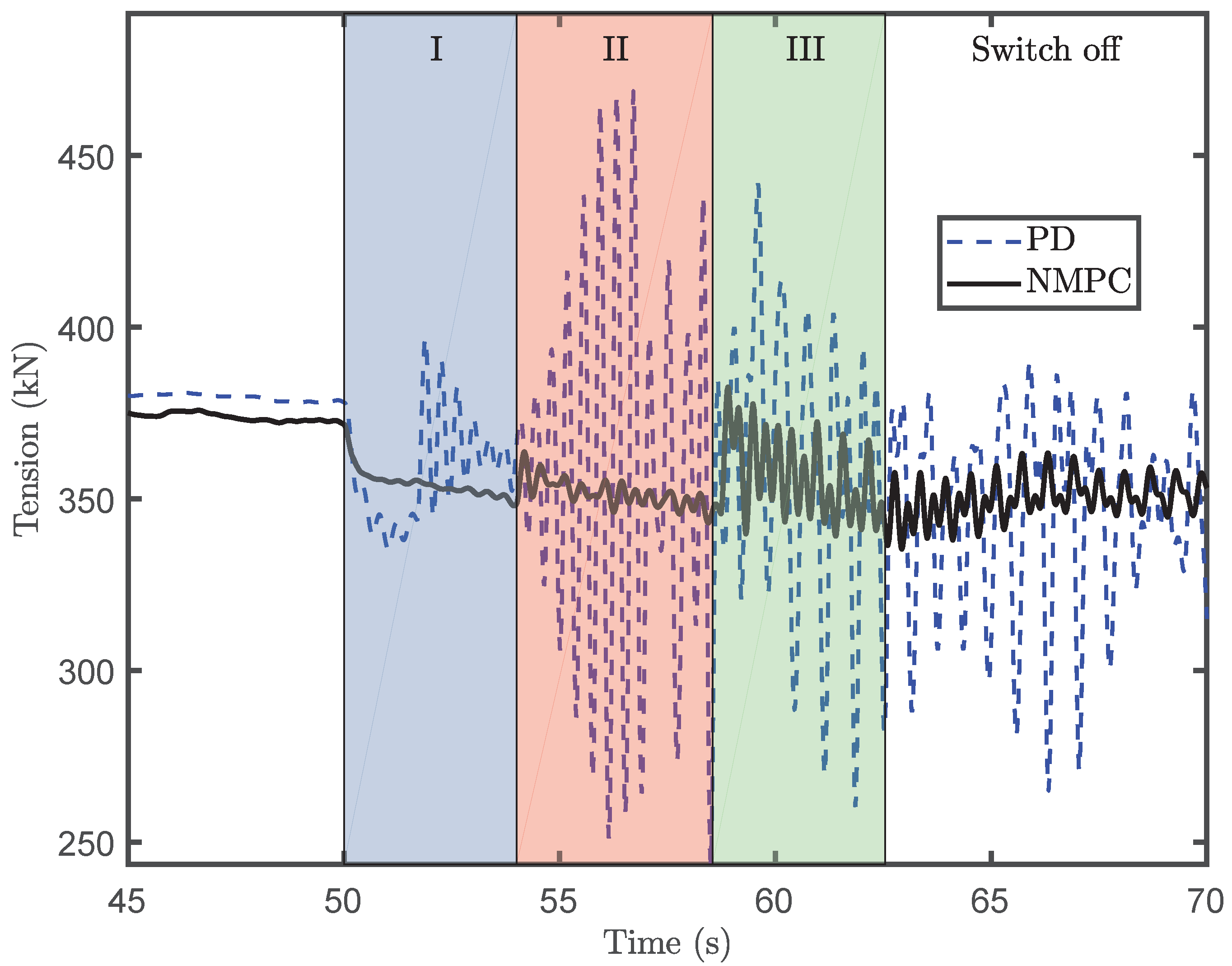
Before the start of the lifting operation, the blade is stabilized by the tugger lines, and the tension oscillation is not remarkable. In Region I, the NMPC controller eliminates most of the oscillation. In Region II, the tension oscillation is caused by interactions between the wind-induced load and the tugger lines. However, the tension oscillation is acceptable in this region. Although the axial tension is not perfectly canceled out in Region III, the NMPC controller performs better than the PD controller. Due to the small wire rope damping ratio, the dynamic tension continues to oscillate after reaching the desired lifting speed. Additionally, because of the higher wind loads, the magnitude of the tension oscillation after the end of the lifting operation increases with higher mean wind speed. It is evident that the amplitude of oscillation is effectively reduced by the proposed NMPC scheme.

The NMPC approach exhibits a superior capacity to regulate the dynamic oscillation, compared to the PD controller. Thus, the NMPC algorithm succeeds to limit winch wear. However, its performance can be further improved, as shown in [37] owing to the simplification of the reduced model.

5.4. Robustness Test of the Algorithm

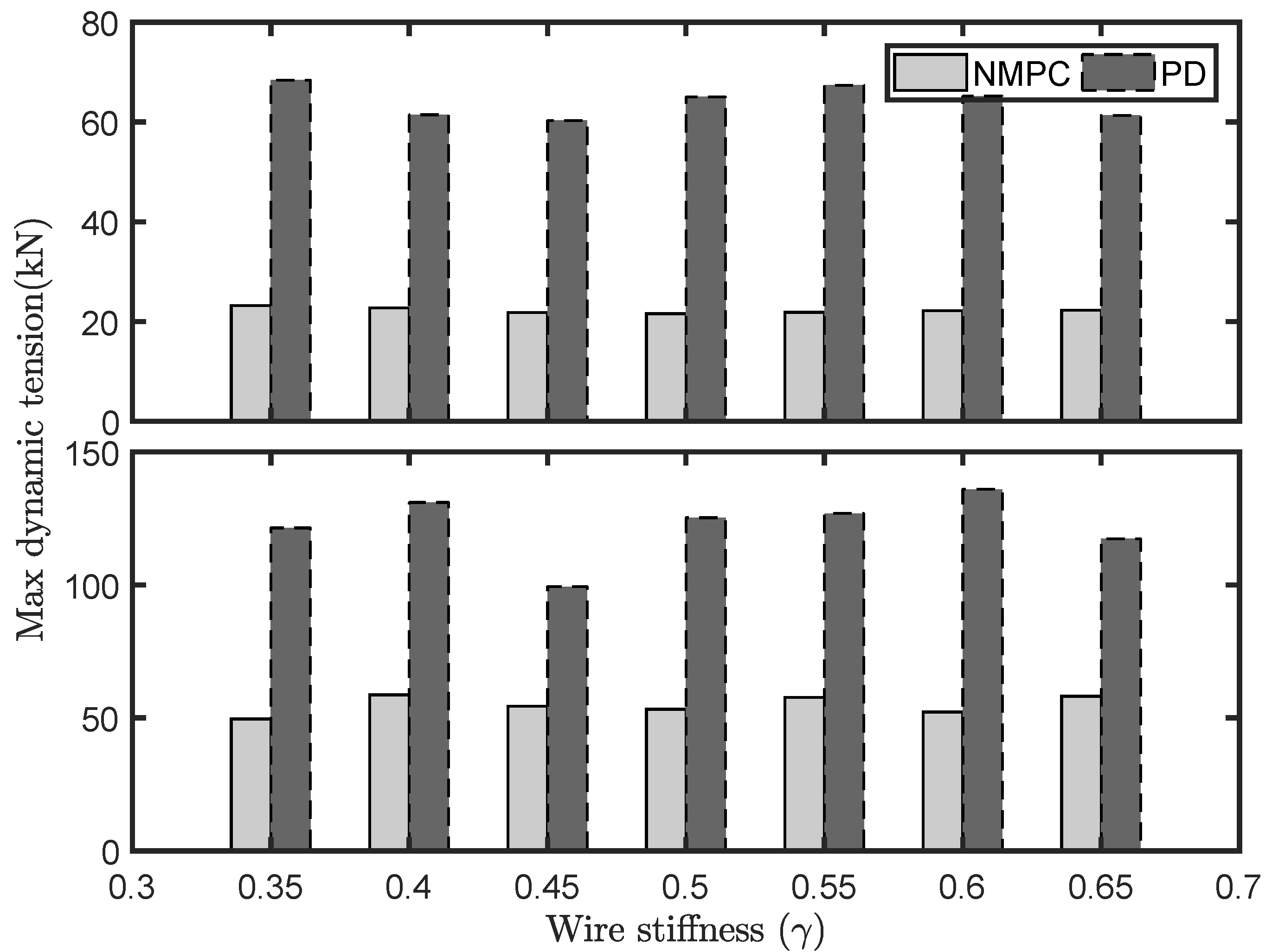
The performance of an NMPC controller is determined by the fidelity of the selected control design model. In our case, the most uncertain parameters are the lift wire stiffness and the neglected wind speed. The effects of model uncertainty matter, as the lift wire stiffness is estimated. Hence, a series of simulations are conducted to test their influence to the controller performance. The wire stiffness is changed by $\gamma =\{0.35,0.4,0.45,0.5,0.55,0.6,0.65\}$, while the $\gamma$ of the NMPC controller remains set at $\gamma =0.5$. The mean wind speed is used as a variable in the simulation, ranges from 4–12 m/s. The corresponding results are presented in Figure 15 and Figure 16.

In Figure 15, we see that the dynamic tension caused by the NMPC controller is almost less than 40% of those resulting from the PD controller. The NMPC controller significantly reduces the dynamic tension at the start and end of a lifting operation, even when the stiffness is not well known. In Figure 16, the performance variation of the PD controller resulted from the increasing stiffness uncertainty increasing significantly, while the performance variation of the NMPC controller is small under the same uncertainties. The mean wind speed does not weaken the NMPC performance, since the mean wind speed does not seem to influence the wire tension considerably. Wind loads are compensated by the tugger lines. Therefore, the robustness of the proposed NMPC law is satisfactory.

5.5. Discussion

We found that the NMPC performance deteriorates with a large sampling interval. In this case, the sampling rate does not satisfy the Nyquist–Shannon sampling theorem if the interval is greater than twice the natural period of the axial oscillation (approximately 0.4 s), i.e., discrete measurements do not approximate the underlying continuous responses. Using shorter sampling and control intervals, not surprisingly, the performance of the control scheme is significantly improved, resulting in more subtle control. Nonetheless, the computation speed depends on the computational capabilities of the measurement and embedded systems. Hence, a trade-off must be made between hardware capabilities and control performance. In the simulation results, we have chosen the sampling period as 0.1 s for this trade-off. The variance in results observed at various lengths of time horizons is limited, as several axial oscillation periods exist in the selected optimal horizon. Therefore, several tension oscillation periods occur over an optimization horizon.

The control effort is determined by the weight matrices in the cost functions. The weights in the Mayer term is more important than the weight values for the end step, since the latter only determines one value among $N+1$ values of the sum operator. The final performance could be prioritized by enhancing it. The running time for the direct multiple shooting approach is longer than that of the direct single shooting approach due to much fewer Karush–Kuhn–Tucker (KKT) conditions involved in the single shooting approach [50]. On the other hand, its application is limited by the strong dependence on the initial guess.

6. Conclusions

An NMPC algorithm is proposed as a mean for efficient and safe lifting operations of a wind turbine blade, by limiting sudden overloads and snatch loads. The simplified model for control design is derived using the Newton–Euler approach. The proposed algorithm has a simple structure. According to the comparative study results, the proposed controller successfully prevents the sudden peak tension, tension dynamics, and the axial oscillation. The NMPC controller still performs well when the lift wire stiffness is poorly estimated or the suspended blade is exposed to a turbulent wind field.

To further improve the system performance when exposed to higher wind speed and model uncertainties, the further research emphasis is on adaptive and robust optimal control schemes, e.g., tube-based model predictive control. In addition, NMPC applications to the blade lifting operation using a floating installation vessel for deep water installation will be investigated.

References

- Jiang, Z.; Hu, W.; Dong, W.; Gao, Z.; Ren, Z. Structural Reliability Analysis of Wind Turbines: A Review. Energies 2017, 10, 2099. [Google Scholar] [CrossRef]
- Jiang, Z.; Gao, Z.; Ren, Z.; Li, Y.; Duan, L. A parametric study on the final blade installation process for monopile wind turbines under rough environmental conditions. Eng. Struct. 2018, 172, 1042–1056. [Google Scholar] [CrossRef]
- Ren, Z.; Jiang, Z.; Skjetne, R.; Gao, Z. An active tugger line force control method for single blade installations. Wind Energy 2018, 21, 1344–1358. [Google Scholar] [CrossRef]
- Ren, Z.; Jiang, Z.; Skjetne, R.; Gao, Z. Development and application of a simulator for Offshore Wind Turbine Blades Installation. Ocean Eng. 2018, 166, 380–395. [Google Scholar] [CrossRef]
- Maes, K.; De Roeck, G.; Lombaert, G. Motion tracking of a wind turbine blade during lifting using RTK-GPS/INS. Eng. Struct. 2018, 172, 285–292. [Google Scholar] [CrossRef]
- Verma, A.S.; Jiang, Z.; Vedvikc, N.P.; Gao, Z.; Ren, Z. Impact assessment of blade root with a hub during the mating process of an offshore monopile-type wind turbine. Eng. Struct. 2018, in press. [Google Scholar]
- Verma, A.S.; Vedvik, N.P.; Haselbach, P.U.; Gao, Z.; Jiang, Z. Comparison of numerical modelling techniques for impact investigation on a wind turbine blade. Compos. Struct. 2019, 209, 856–878. [Google Scholar] [CrossRef]
- Abdel-Rahman, E.M.; Nayfeh, A.H.; Masoud, Z.N. Dynamics and control of cranes: A review. J. Vib. Control 2003, 9, 863–908. [Google Scholar] [CrossRef]
- Spathopoulos, M.; Fragopoulos, D. Pendulation control of an offshore crane. Int. J. Control 2004, 77, 654–670. [Google Scholar] [CrossRef]
- Schaub, H. Rate-based ship-mounted crane payload pendulation control system. Control Eng. Pract. 2008, 16, 132–145. [Google Scholar] [CrossRef]
- He, W.; Zhang, S.; Ge, S.S. Adaptive control of a flexible crane system with the boundary output constraint. IEEE Trans. Ind. Electron. 2014, 61, 4126–4133. [Google Scholar] [CrossRef]
- d’Andréa Novel, B.; Coron, J.M. Exponential stabilization of an overhead crane with flexible cable via a back-stepping approach. Automatica 2000, 36, 587–593. [Google Scholar] [CrossRef]
- Sun, N.; Fang, Y.; Zhang, X. Energy coupling output feedback control of 4-DOF underactuated cranes with saturated inputs. Automatica 2013, 49, 1318–1325. [Google Scholar] [CrossRef]
- Tang, R.; Huang, J. Control of bridge cranes with distributed-mass payloads under windy conditions. Mech. Syst. Signal Process. 2016, 72, 409–419. [Google Scholar] [CrossRef]
- Johansen, T.A.; Fossen, T.I.; Sagatun, S.I.; Nielsen, F.G. Wave synchronizing crane control during water entry in offshore moonpool operations-experimental results. IEEE J. Ocean. Eng. 2003, 28, 720–728. [Google Scholar] [CrossRef]
- Skaare, B.; Egeland, O. Parallel force/position crane control in marine operations. IEEE J. Ocean. Eng. 2006, 31, 599–613. [Google Scholar] [CrossRef]
- Messineo, S.; Serrani, A. Offshore crane control based on adaptive external models. Automatica 2009, 45, 2546–2556. [Google Scholar] [CrossRef]
- Jiang, Z.; Ren, Z.; Gao, Z.; Sandvik, P.C.; Halse, K.H.; Skjetne, R. Mating Control of a Wind Turbine Tower-Nacelle-Rotor Assembly for a Catamaran Installation Vessel. In Proceedings of the 28th International Ocean and Polar Engineering Conference, Sapporo, Japan, 10–15 June 2018; pp. 584–593. [Google Scholar]
- Yang, T.; Yang, X.; Chen, F.; Fang, B. Nonlinear parametric resonance of a fractional damped axially moving string. J. Vib. and Acoustics 2013, 133, 064507. [Google Scholar] [CrossRef]
- Bemporad, A.; Morari, M. Robust model predictive control: A survey. In Robustness in Identification and Control; Springer: London, UK, 1999; pp. 207–226. [Google Scholar]
- Kellett, C.M.; Teel, A.R. Smooth Lyapunov functions and robustness of stability for difference inclusions. Syst. Control Lett. 2004, 52, 395–405. [Google Scholar] [CrossRef]
- Adetola, V.; DeHaan, D.; Guay, M. Adaptive model predictive control for constrained nonlinear systems. Syst. Control Lett. 2009, 58, 320–326. [Google Scholar] [CrossRef]
- Mayne, D.Q.; Kerrigan, E.C.; Van Wyk, E.; Falugi, P. Tube-based robust nonlinear model predictive control. Int. J. Robust Nonlinear Control 2011, 21, 1341–1353. [Google Scholar] [CrossRef]
- Mayne, D.Q. Model predictive control: Recent developments and future promise. Automatica 2014, 50, 2967–2986. [Google Scholar] [CrossRef]
- Deng, W.; Yao, R.; Zhao, H.; Yang, X.; Li, G. A novel intelligent diagnosis method using optimal LS-SVM with improved PSO algorithm. Soft Comput. 2017, 161, 1–18. [Google Scholar] [CrossRef]
- Mayne, D.Q.; Rawlings, J.B.; Rao, C.V.; Scokaert, P.O. Constrained model predictive control: Stability and optimality. Automatica 2000, 36, 789–814. [Google Scholar] [CrossRef]
- Diehl, M.; Findeisen, R.; Allgöwer, F.; Bock, H.G.; Schlöder, J.P. Nominal stability of real-time iteration scheme for nonlinear model predictive control. IEE Proc. Control Theory Appl. 2005, 152, 296–308. [Google Scholar] [CrossRef] [Green Version]
- Diehl, M.; Bock, H.G.; Schlöder, J.P. A real-time iteration scheme for nonlinear optimization in optimal feedback control. SIAM J. Control Optim. 2005, 43, 1714–1736. [Google Scholar] [CrossRef]
- Zhu, M.; Hahn, A.; Wen, Y.; Bolles, A. Identification-based simplified model of large container ships using support vector machines and artificial bee colony algorithm. Appl. Ocean Res. 2017, 68, 249–261. [Google Scholar] [CrossRef]
- Zhu, M.; Hahn, A.; Wen, Y. Identification-based controller design using cloud model for course-keeping of ships in waves. Eng. Applic. Artific. Intell. 2018, 75, 22–35. [Google Scholar] [CrossRef]
- Niu, H.; Lu, Y.; Savvaris, A.; Tsourdos, A. An energy-efficient path planning algorithm for unmanned surface vehicles. Ocean Eng. 2018, 161, 308–321. [Google Scholar] [CrossRef]
- Andersson, J. A General-Purpose Software Framework for Dynamic Optimization. Ph.D. Thesis, Arenberg Doctoral School, KU Leuven, Department of Electrical Engineering (ESAT/SCD) and Optimization in Engineering Center, Heverlee, Belgium, 2013. [Google Scholar]
- Ariens, D.; Houska, B.; Ferreau, H.; Logist, F. ACADO for Matlab User’s Manual; Optimization in Engineering Center (OPTEC): Wetzikon, Switzerland, 2010; Available online: http://www.acadotoolkit.org (accessed on 19 November 2017).
- Mattingley, J.; Boyd, S. CVXGEN: A code generator for embedded convex optimization. Optim. Eng. 2012, 13, 1–27. [Google Scholar] [CrossRef]
- Ren, Z.; Jiang, Z.; Skjetne, R.; Gao, Z. Single blade installation using active control of three tugger lines. In Proceedings of the 28th International Ocean and Polar Engineering Conference, Sapporo, Japan, 10–15 June 2018; pp. 594–601. [Google Scholar]
- Ren, Z.; Skjetne, R.; Jiang, Z.; Gao, Z.; Verma, A.S. Integrated GNSS/IMU Hub Motion Estimator for Offshore Wind Turbine Blade Installation. Mech. Syst. Signal Process. 2019. Revision. [Google Scholar]
- Ren, Z.; Skjetne, R.; Gao, Z. Modeling and Control of Crane Overload Protection during Marine Lifting Operation Based on Model Predictive Control. In Proceedings of the ASME 2017 36th International Conference on Ocean, Offshore and Arctic Engineering, Trondheim, Norway, 25–30 June 2017; p. V009T12A027. [Google Scholar]
- Espinoza, A. Block Island Wind Farm Enters Final Construction Phase. 2016. Available online: http://ripr.org/post/block-island-wind-farm-enters-final-construction-phase#stream/0 (accessed on 19 November 2017).
- Jonkman, J.; Butterfield, S.; Musial, W.; Scott, G. Definition of a 5-MW Reference Wind Turbine for Offshore System Development; Technical Report No. NREL/TP-500-38060; National Renewable Energy Laboratory: Golden, CO, USA, 2009.
- Fossen, T.I. Handbook of Marine Craft Hydrodynamics and Motion Control; John Wiley & Sons: Hoboken, NJ, USA, 2011. [Google Scholar]
- Todd, M.; Vohra, S.; Leban, F. Dynamical measurements of ship crane load pendulation. In Proceedings of the OCEANS’97, MTS/IEEE Conference Proceedings, Halifax, NS, Canada, 6–9 October 1997; Volume 2, pp. 1230–1236. [Google Scholar]
- Wächter, A. Short Tutorial: Getting Started with Ipopt in 90 Minutes; Dagstuhl Seminar Proceedings, Schloss Dagstuhl-Leibniz-Zentrum für Informatik: Wadern, Germany, 2009. [Google Scholar]
- Johansen, T.A. Introduction to nonlinear model predictive control and moving horizon estimation. Sel. Top. Constrained Nonlinear Control 2011, 1–53. [Google Scholar] [CrossRef]
- Vukov, M.; Domahidi, A.; Ferreau, H.J.; Morari, M.; Diehl, M. Auto-generated algorithms for nonlinear model predictive control on long and on short horizons. In Proceedings of the 52nd IEEE Conference on Decision and Control, Florence, Italy, 10–13 December 2013; pp. 5113–5118. [Google Scholar]
- Deng, W.; Zhao, H.; Zou, L.; Li, G.; Yang, X.; Wu, D. A novel collaborative optimization algorithm in solving complex optimization problems. Soft Comput. 2017, 21, 4387–4398. [Google Scholar] [CrossRef]
- Deng, W.; Zhao, H.; Yang, X.; Xiong, J.; Sun, M.; Li, B. Study on an improved adaptive PSO algorithm for solving multi-objective gate assignment. Appl. Soft Comput. 2017, 59, 288–302. [Google Scholar] [CrossRef]
- Chen, H.; Allgower, F. A Quasi-infinite Horizon nonlinear model predictive control scheme with guaranteed stability. In Proceedings of the IEEE European Control Conference, Brussels, Belgium, 1–7 July 1997; pp. 1421–1426. [Google Scholar]
- Zhou, L.; Moan, T.; Riska, K.; Su, B. Heading control for turret-moored vessel in level ice based on Kalman filter with thrust allocation. J. Mar. Sci. Technol. 2013, 18, 460–470. [Google Scholar] [CrossRef]
- Wind Turbine Generator Systems-Part 1: Safety Requirements; Standard, International Electrotechnical Commission: Geneva, Switzerland, 2005.
- Luo, Z.Q.; Yu, W. An introduction to convex optimization for communications and signal processing. IEEE J. Sel. Areas Commun. 2006, 24, 1426–1438. [Google Scholar] [Green Version]
Figure 1.
Single blade installation (Image source: RIPR [38]).
Figure 2.
Free body diagram of the blade lifting operation.
Figure 3.
The lift wire tension history of a suspended blade with constant lifting-off speeds.
Figure 4.
The lift wire tension history of a suspended blade with constant lowering speeds.
Figure 5.
Example of the lifting problem in different regions.
Figure 6.
Illustration of direct multiple shooting.
Figure 7.
An example of the normalizing weights for Region I with respect to the subinterval number.
Figure 8.
An example of the normalizing weights for Region III with respect to the subinterval number.
Figure 9.
Block diagram of the hybrid control scheme.
Figure 10.
Performance of the PD controller with saturating elements and NMPC controller.
Figure 11.
The field voltage, , mean wind speed 0 m/s, .
Figure 12.
Comparison of the time-domain simulation results of the tension on the lift wire, , mean wind speed 0 m/s, .
Figure 13.
Comparison of the time-domain simulation results of the tension on the lift wire, , mean wind speed 8 m/s, .
Figure 14.
Comparison of the time-domain simulation results of the tension on the lift wire, , mean wind speed 12 m/s, .
Figure 15.
Comparison of the maximum dynamic tensions resulted by the NMPC and PD controllers, mean wind speed = 0 m/s (upper: Region I, lower: Region III).
Figure 16.
Comparison of the maximum dynamic tensions resulted by the NMPC and PD controllers in a turbulent wind field, mean wind speed = 4–12 m/s (upper: Region I, lower: Region III).