2.1. Posterior Predictive Process
Gaussian processes give rise to a class of Bayesian nonparametric models which have garnered tremendous attention in the machine learning community. The recent attention belies the fact that Gaussian processes, and more broadly kernel methods, have been used in scientific computing and numerical analysis for over 70 years. These methods draw on a rich theoretical and practical background. The popularity of Gaussian processes is due to the flexibility of modeling in infinite-dimensional space, the efficiency with which the data are used, the ease of implementation, and the natural handling of uncertainty. These properties make Gaussian processes ideal to forecast load for energy trading where accurate point estimates are required and uncertainty (i.e., risk) quantification is desirable.
Consider a matrix of input data
such that
, and
are column vectors. For this paper, the input data consist of temperatures
, dew points
, and a time component
, such that for
,
Output data, load, are also observed,
such that
. The goal is to predict the load,
, at
future times given future inputs
. For Gaussian processes, the posterior distribution of the predictive process relies on the particular positive definite kernel chosen for the task; the properties of various kernels are discussed in
Section 2.3. For shorthand, it is a common abuse of notation to pass the kernel matrix-valued arguments; the corresponding output is a kernel matrix (often referred to as the Gram matrix), as discussed in
Appendix A. The posterior process is derived in [
16], and the result is that
, when conditioned on the observed data
is Gaussian distributed. This is denoted as follows:
where
is the posterior mean,
and
is the posterior variance,
The mean term is also referred to as the maximum a posteriori (MAP) estimate. In our context, it is a point forecast of the load. Sample realizations can be drawn from the predictive distribution, providing a mathematically rigorous and computationally efficient estimate of uncertainty. As a density estimate for future load, the posterior distribution can be used downstream in electricity price forecasting and modeling the risk associated with generation or trading decisions.
2.3. Properties of Positive Definite Kernels
Equations (
1) and (
3) make clear that the problem of modeling in a Gaussian process framework revolves around the positive definite kernel
K, and its kernel matrix
. A brief mathematical background on positive definite kernels is provided in the Appendix. Gaussian processes are
nonparametric models due to the fact that parameters do not appear in the model (see, for instance, Equation (
1)). This nomenclature is somewhat confusing as the kernel itself is typically parameterized. The parameterization of the kernel is important to the modeling process; it allows the analyst to impose structure on the covariance (to specify, for instance, periodicity), and allows for intuitive interpretations of the model. In the statistics literature, a positive definite kernel is referred to as a
covariance kernel, emphasizing that
is a covariance function. Evaluating this function at particular arguments,
, provides the covariance between two points
and
; performing this operation for
and
yields the kernel matrix
. The goal is to identify the correct covariance structure of the data by selecting an appropriate kernel and parameterizing it correctly. Since the choice of kernel and its parameterization determine the properties of the model, making an appropriate selection is crucial. In this section, we provide examples of the kernels used in our model, explain the rationale behind their use, and discuss mathematical properties needed to construct the model from these kernels.
The most obvious structure of the data is the cyclic nature over the course of the day, week, and year. A discussion of the 7- and 365-day seasonality can be found in [
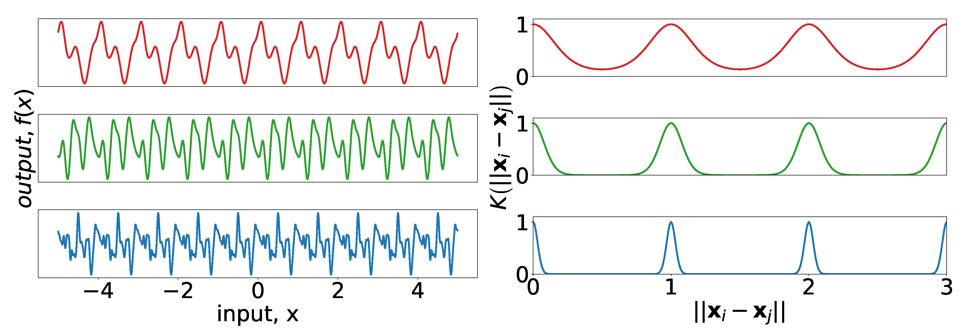
28], where the authors showed load data in the frequency domain to identify the cyclic behavior. Their analysis has intuitive appeal as it confirms the seasonal structure of power demand one might expect before observing any data. The periodic kernel, first described in [
29], can be used to model seasonality:
where
are the amplitude, the period, and the length-scale, respectively.
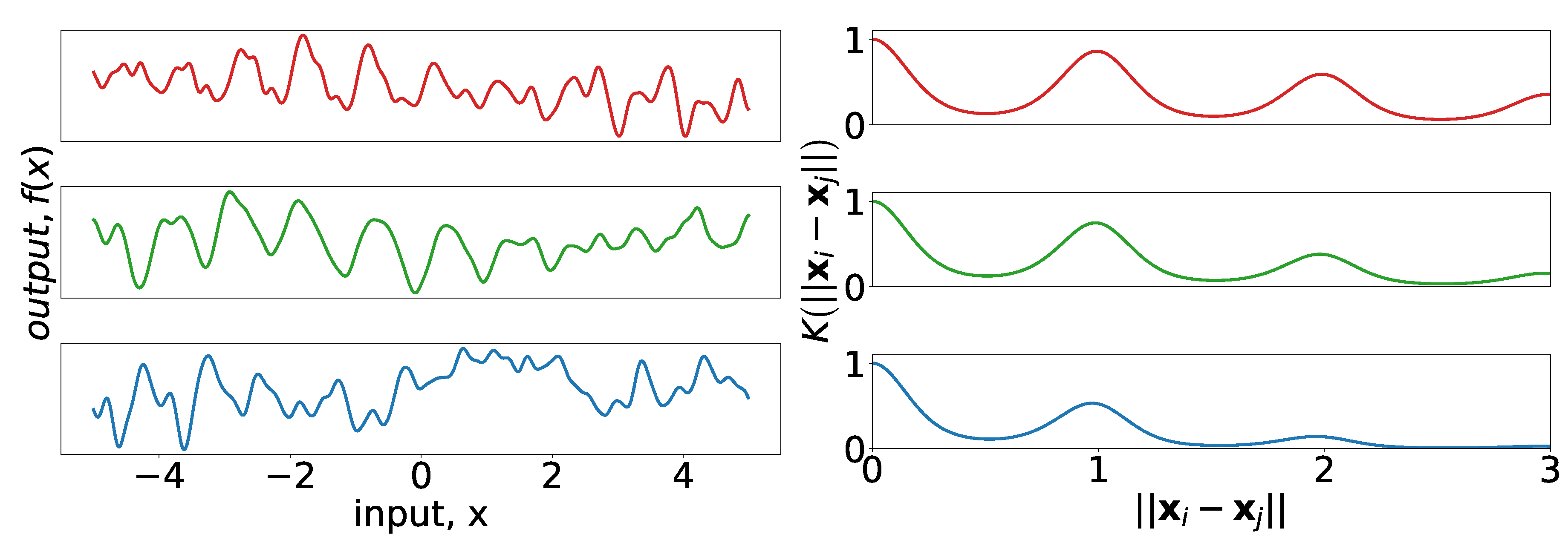
Figure 4 provides examples of periodic kernels of different length-scales, as well as realizations of Gaussian processes drawn using the kernels as covariance functions.
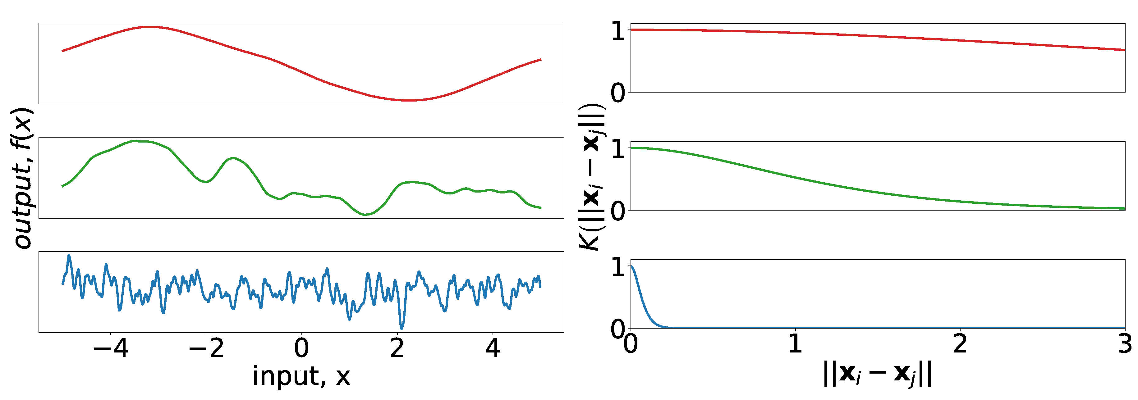
The Gaussian (also known as squared-exponential) kernel is commonly used in the machine learning literature. It has the form
where in this context
are the amplitude and length-scale parameters, respectively.
Figure 5 provides insight into the effect of the length-scale parameter for the Gaussian kernel. Notice that the samples in all cases are smooth even for short length-scales, which is characteristic of the Gaussian kernel.
The Matérn 5/2 kernel, commonly used in the spatial statistics literature, has the form
Here,
are the amplitude and length-scale parameters, respectively, which are analogous to their counterparts in the Gaussian and periodic kernels. The general Matérn kernel can be viewed as a generalization of the covariance function of the Ornstein–Uhlenbeck (OU) process to higher dimensions ([
16] Section 4.2). The OU process has been used before to forecast load (see, e.g., [
30]), although in a different context then we use the Matérn here.
Figure 6 provides insight into the effect of the length-scale parameter for the Matérn 5/2 kernel. Although
Figure 6 (right) appears almost indistinguishable from the corresponding frame of
Figure 5, it is apparent in
Figure 6 (left) that draws from Gaussian processes with the Matérn kernel are not smooth (though they are twice-differentiable).
At this point, we have introduced several kernels, but the posterior predictive distribution outlined in
Section 2.1 only identifies a single kernel. The following properties of positive definite kernels allow for their combination:
Remark 1. Let be two positive definite kernels taking arguments from a vector space . Then, for all :
is a positive definite kernel.
is a positive definite kernel.
Furthermore, if takes arguments from (for instance, time), takes arguments from (for instance, space). Then, for all in and all in :
is a positive definite kernel.
is a positive definite kernel.
Proofs of the statements in the above remark are straightforward and can be found in ([
31] Section 13.1). This remark allows for the combination of all the kernels that have been discussed in a way that is intuitive and easy to code. For example, we use the periodic kernel with a Matérn decay on time:
The kernel can be interpreted as follows: the Matérn portion allows for a decay away from strict periodicity. This allows the periodic structure to change with time. A small length-scale for
corresponds to rapid changes in the periodic structure, whereas a long length-scale would suggest that the periodicity remains constant over long periods of time. We combine the amplitude parameters of each kernel into a single parameter,
.
Figure 7 demonstrates the effect that varying
of Equation (
7) has on the kernel, and on realizations of a process using that kernel. Consider that the structure of the top realization in
Figure 7 (left) has clear similarities between successive periods, but after four or five periods the differences become more pronounced; this is in contrast to the bottom realization for which the similarities after two periods are already difficult to identify.
2.4. Creating a Composite Kernel for Load Forecasts
To showcase the properties of this method, and to give insight into how one might go about creating a composite kernel using domain expertise, we step through the construction of one such kernel in this section. At each step, we discuss the desired phenomena that we would like to capture with the structure of the latest model. We also provide figures to help interpret the effect the changes have on the resulting predictions. The purpose of this section is to demonstrate how practitioners and researchers can create kernels which incorporate their own understanding of the ways load can vary with the forecast inputs. For illustrative purposes, we use the same training/test data for every step in this process.
We train each model on PJMISO data beginning on 17 September 2018 and ending on 26 October 2018. We then predict load for 27 October 2018. The point estimate prediction is the posterior mean of the Gaussian process. We also draw 1000 samples from the posterior distribution to illustrate the uncertainty of the model. Parameters that are not set manually are estimated via maximum likelihood, as described in
Section 2.5. The parameter
is not associated with any kernel, but reflects the magnitude of the noise, and is required for regularizing the kernel, as shown in Equations (
1) and (
3).
We begin with two kernels meant to capture the periodicity. As discussed in
Section 2.3, there is known daily and weekly seasonality to the data, thus we fixed the parameters that control the period. The kernel is thus,
where
is the amplitude of the composite kernel. The parameters are provided in
Table 1.
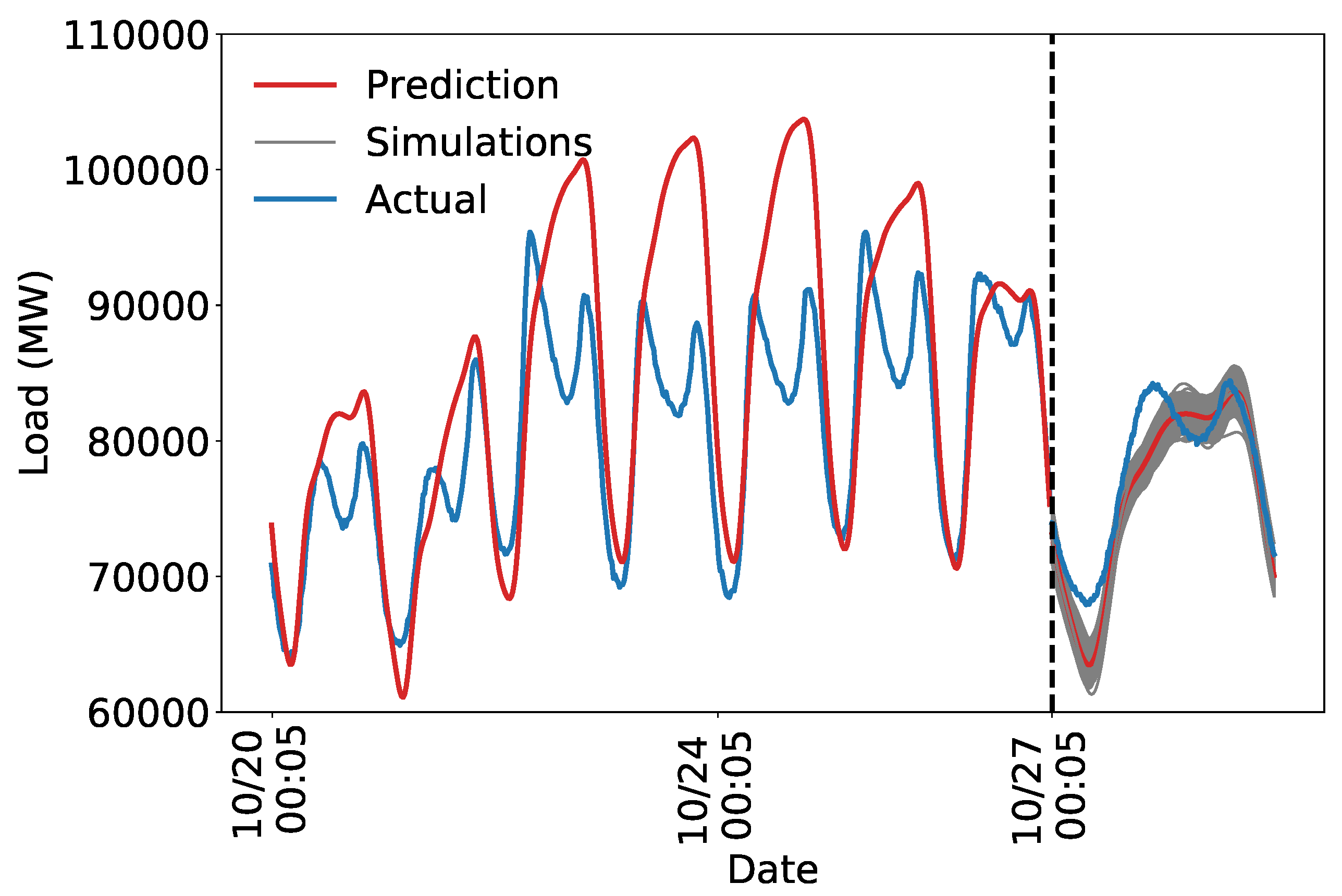
Figure 8 shows that the daily and weekly periodicity capture a substantial portion of the variation in load. As expected, a purely periodic structure is not sufficient to accurately predict future load. Nevertheless, capturing the weekly and daily periodicity is an important first step for creating an accurate model. The estimated uncertainty is too low, likely because the model is not flexible enough to capture all the variation in load. We next develop a kernel that specifies a more realistic model to address this problem.
Studying the structure of the forecasted and actual data in
Figure 8 suggests that a decay away from exact periodicity is desirable. One way to achieve this is via the kernel described in Equation (
7). In particular, we want to allow consecutive days to co-vary more strongly than nonconsecutive days, and similarly for weeks. This structure is described in Equation (
9) and
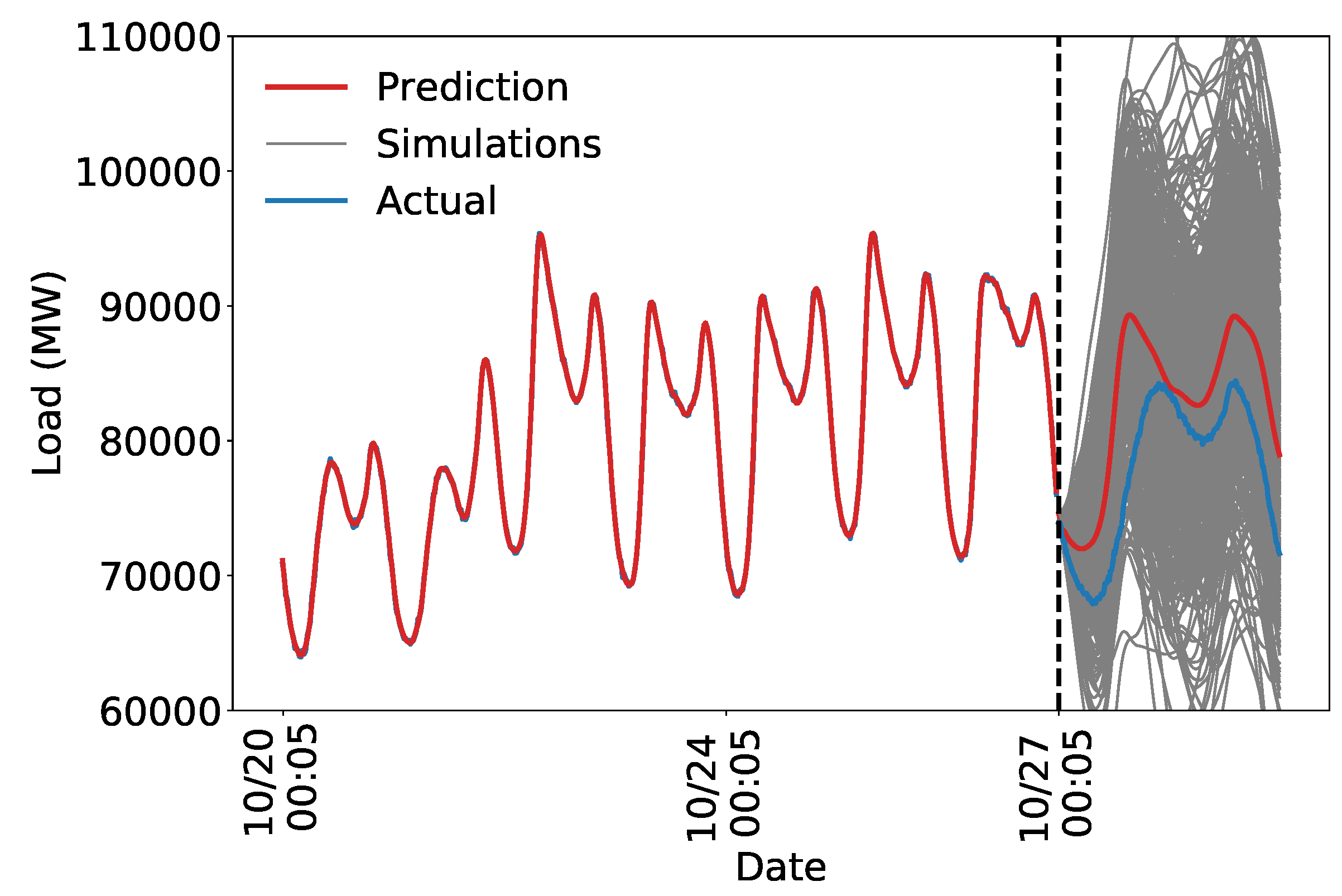
Table 2Relaxing the strict periodic structure gives the model the flexibility required to capture the shape of the load curve. The noise term regularizes as needed to avoid overfitting. The training set is nearly perfectly predicted, but the model seems to generalize adequately, suggesting the regularization is working.
Figure 9 shows that the decaying periodic model better captures the structure of the load, and the uncertainty is more realistic. The predicted uncertainty is too high which we address by adding more structure to the model.
The model appears to explain the temporal trends in the training data. For example, note the distinct dip and rise in the test predictions around the morning peak, characteristic of an autumn load curve. The discrepancy between the forecast and actual values on the test set may be due to the inability of a strictly time series model to capture all of the intricacies of power demand on the electric grid.
A reasonable next step is to incorporate temperature information. We do this with a tensor product over time to allow for a decay of the relevance of information as time passes. The resulting kernel is described by Equation (
10) with the parameters outlined in
Table 3. The temperature data are modeled with a single Gaussian kernel, which gives changes in temperature at every location equal weight. More sophisticated methods for handling the high-dimensional temperature data are discussed in
Section 2.6.
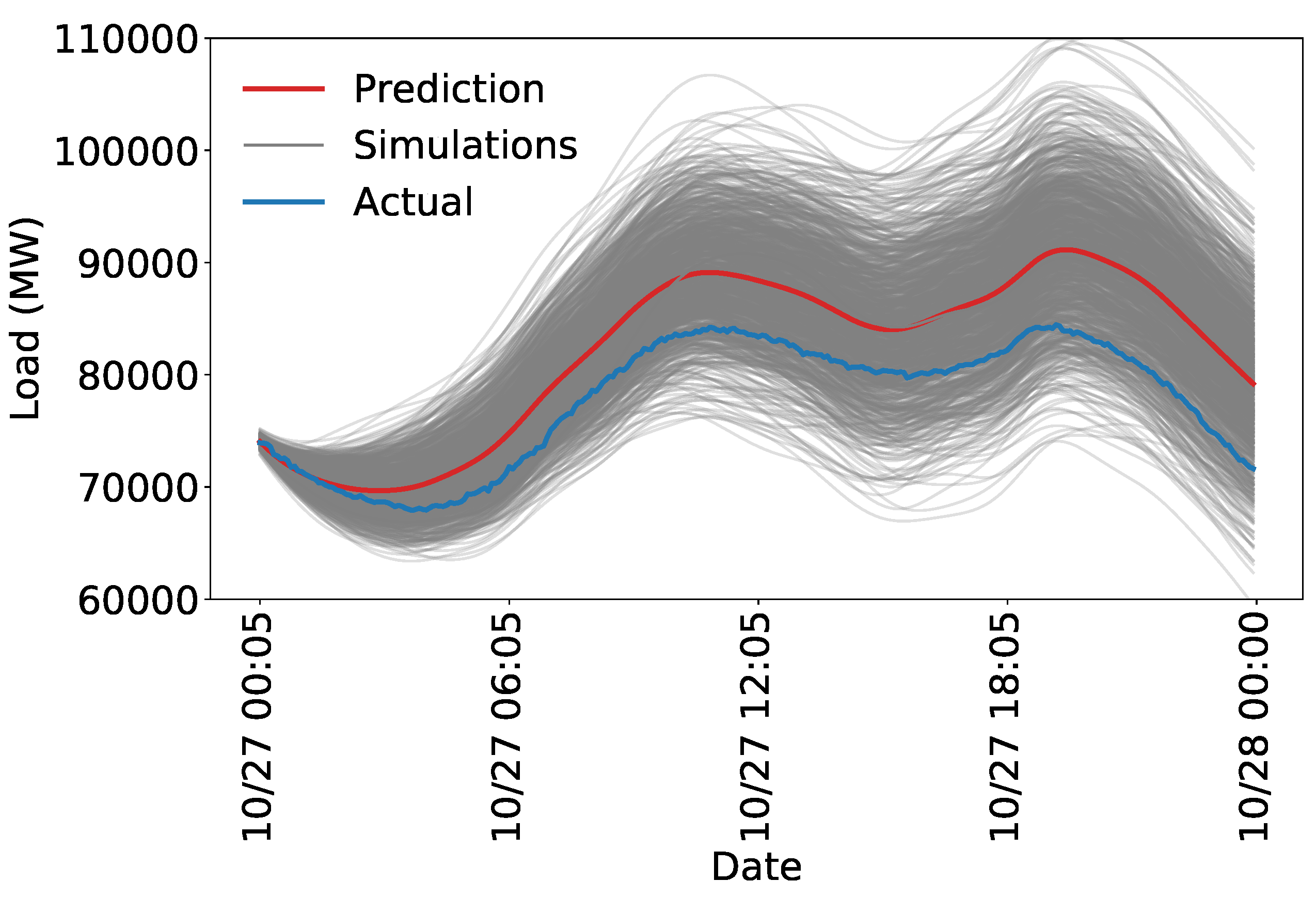
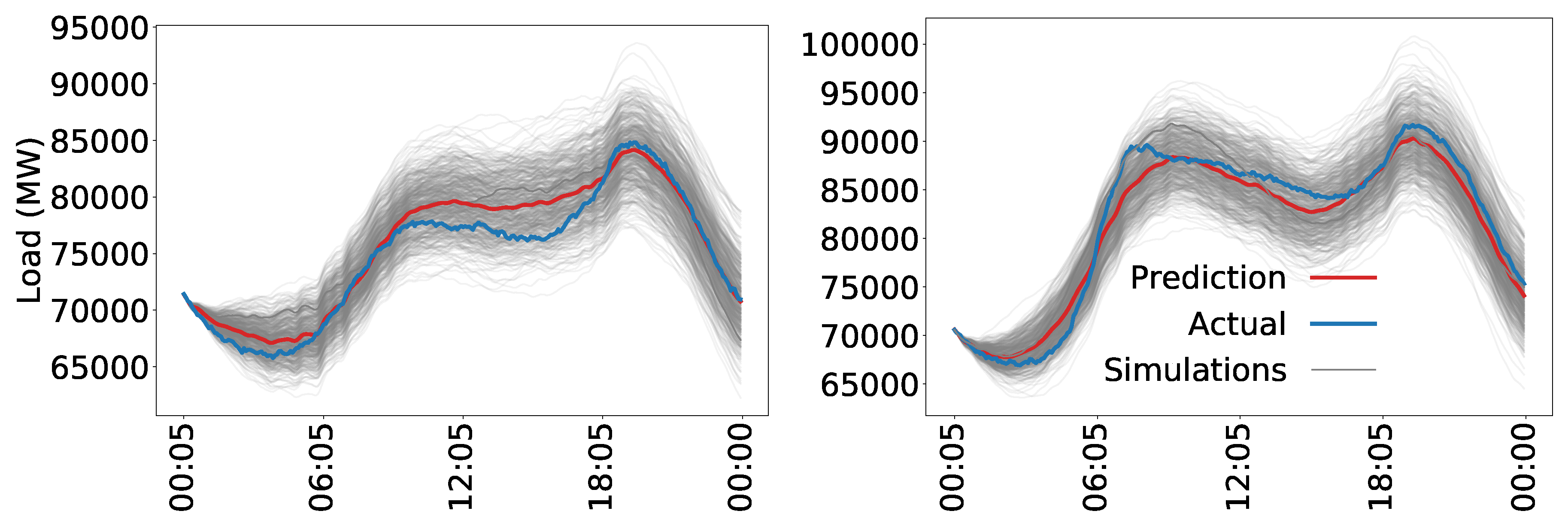
Figure 10 shows the results of using the kernel to predict only on the test set. The simulations shown in
Figure 10 are more accurate than those shown in
Figure 9. The errors are smaller and the uncertainty appears more reasonable. Clearly, some phenomena are not picked up by the model. There remains a persistent error of approximately 5000 MW throughout the day. A more rigorous evaluation of the performance and a more thorough analysis of the forecast error and uncertainty for more complex models is provided in
Section 3.
The model used in
Section 3 is the result of creating a composite kernel using the procedure described in this section. The final kernel includes additional structure meant to capture phenomena not discussed in this section. In contrast to many modern machine learning techniques, we develop this structure consistent with domain specific knowledge as described above. The ability to incorporate this type of knowledge makes Gaussian processes among the most powerful tools available to researchers with subject expertise. The benefits of Gaussian processes are likely smaller for situations where the modeler has little domain specific knowledge.
2.5. Parameter Estimation
Once the kernel has been specified, the values of the parameters of the model must be determined. We use maximum likelihood estimation, a popular and mathematically sound method for parameter estimation. The log marginal likelihood of a Gaussian process is
where the parameter vector
is implicit in the kernel and
det is the determinant of the matrix. The observed data are fixed, thus the goal is to choose the parameters which are most likely to have resulted in the observed data. Equation (
11) has a convenient interpretation that helps explain why Gaussian processes are useful for modeling complex phenomena: the first term is the data-fit, encapsulating how well the kernel evaluated at the inputs represents the outputs. The second term is a penalty on the complexity of the model, depending only on the covariance function and the inputs. The third term is a normalization constant. Maximum likelihood estimation of the Gaussian process occurs over the hyperparameters
and the complexity penalty inherently regularizes the solution.
Likelihood maximization is an optimization problem that can be tackled in a variety of ways. Due to the high-dimensionality of the problem, a grid search is too time consuming. For the forecasts in
Section 3, we use a generalization of gradient descent called stochastic subspace descent, as described in [
32] and defined in Algorithms 1 and 2.
| Algorithm 1 Generate a scaled Haar distributed matrix (based on [33]). |
Inputs: ▹ Dimensions of desired matrix, Outputs: such that: columns of are orthogonal Initialize Set Calculate QR decomposition of Let P =
|
Algorithm 2 is called by passing a random initialization of the parameters as well as a step-size, and a parameter
ℓ which dictates the rank of the subspace that is used for the descent. The generic function
that Algorithm 2 minimizes is specified by Equation (
11).
| Algorithm 2 Stochastic subspace descent. |
Inputs: ▹ step size, subspace rank Initialize: for k = 1, 2, … do Generate by Algorithm 1 end for
|
This particular optimization routine is designed for high-dimensional problems with expensive function evaluations and gradients that are difficult or impossible to evaluate. Stochastic subspace descent uses finite differences to compute directional derivatives of low-dimensional random projections of the gradient in order to reduce the computational burden of calculating the gradient. The subroutine in Algorithm 1 defines a random matrix that is used to determine which directional derivatives to compute. Automatic differentiation software such as
autograd for Python [
34] can speed up the implementation by removing the need for finite differences, or, for simpler kernels, the gradients can be calculated by hand. For complex kernels, this may not be feasible so for generality and programming ease we use a zeroth-order method.
An important attribute of stochastic subspace descent is that the routine avoids getting caught in saddle points which is a typical problem in high-dimensional, non-convex optimization as discussed in [
35]. Despite the fact that this algorithm avoids saddle points, there is no guarantee that the likelihood surface is convex for any particular set of data and associated parameterization. Non-convexity implies that there may be local maxima with suboptimal likelihood that are far from the global maximum in parameter space. To address this concern, we perform multiple restarts of the optimization routine with the parameters initialized randomly over the domain.
2.7. Model Combination
Ensemble methods, which combine multiple models to create a single more expressive model, have been common in the machine learning community for many years, see [
42] for an early review in the context of classification. Recently, such methods have been applied successfully to load forecasting; in a paper analyzing the prestigious M4 load forecasting competition [
43], model combination is touted as one of the most important tools available to practitioners. Done correctly, models can be created and combined without substantial additional computational overhead. This is due to the parallel nature of many ensembles and is true of our proposed method. Several strategies exist for combining models, particularly in the Bayesian framework which allows for a natural weighting of different models by the
model evidence ([
44] Section 3.4), which in our case is expressed by (
11). Extensive research has been conducted into the combination of Gaussian process models, a comparison of various methods is provided in [
24]. In this paper, we propose using the Generalized Product of Experts (GPoE) method originally described in [
45].
The standard product of experts (PoE) framework [
46] can take advantage of the Gaussian nature of the posterior process. We recall the posterior density from Equation (
1) with an additional subscript to denote the model index
The product of Gaussian densities remains Gaussian, up to a constant:
where
M is the number of models to be combined. The density of the PoE model is
Although Equation (
12) may look complicated, it has a simple interpretation. We can re-write the mean as
, where
is a weight matrix for the
jth model, corresponding to the inverse of the uncertainty of that model. That is, models for which the uncertainty is high are down-weighted compared to those with low uncertainty. The variance
can readily be seen as the inverse of the sum of the constituent precision matrices
.
It is apparent that models with low uncertainty will dominate
, and cause the variance of the PoE model to be relatively small. This is because if
is small, then
will be large, dominating the variance of the other models in the sum. The GPoE framework is designed to ameliorate this by allocating additional weight to those models for which the data are most informative to the model. The details of the algorithm, including how we measure the informativeness of data to a model, are available in
Appendix B. See [
45] for a more detailed discussion.
There is a trade-off to model combination. On the one hand, it is straightforward to implement, provides empirically and provably better estimates (see, e.g., [
42] for a straightforward explanation in the context of classification), and has enormous practical value as demonstrated in the M4 competition. The cost of these benefits is that there is no longer a single kernel to provide interpretability. Since the method for combining the models is to take a product of the densities, the kernels of the individual models get lost in the mix, turning the GPoE model into a black box. Depending on the application, interpretability may or may not be a relevant consideration. The ability to combine models in this way provides the data analyst the opportunity to make a decision based on the requirements placed on the forecast.


