1. Introduction
For many years fossil fuels have been the primary source of energy in the world, however these resources are finite. The threat of climate change due to global warming (caused in part by the burning of fossil fuels) has prompted the search for renewable energy sources such as the sun and the wind. Solar energy is a sustainable, environmentally friendly, and cost-efficient source of energy available around the world, and for this reason solar technologies using photovoltaic (PV) systems have penetrated the electric power production market, with the additional advantages of working quietly and with low maintenance cost. Nonetheless, as it has been remarked by [
1], the increment in the use of PV devices in power systems has generated new challenges, such as those related with control strategies looking to provide good, even optimal, operating conditions of the PV systems. Moreover, the control strategies need to cope with the fact that the performance of PV systems depends on solar irradiance, ambient temperature, and load impedance [
2]. As in [
1], the approach proposed in this paper is implemented in the open programming environment MATLAB
®/Simulink
®; nevertheless, the focused problem is the application of a novel control strategy (flatness-based) for the MPPT in PV systems. As mentioned in [
3], it is evident that PV components will be essential elements in power electrical systems, where their inclusion considers the MPPT control problem as a strategy that is part of one of the two most important approaches highlighted in literature that corresponds to “the installation and operation of an energy storage system (ESS), while keeping the PVs in the maximum power point tracking (MPPT)…” [
3]. To the best knowledge of the authors, no flatness-based control strategies have been reported to cope with the MPPT problem in PV systems. This paper proposes the use of a control strategy based on the differential flatness properties of the PV system model to tackle the MPPT task.
The main drawback of PV systems is their low conversion efficiency. For an optimal operation, it is required for the system to operate at the Maximum Power Point (MPP), which represents the maximum energy that can be extracted from the PV panel. To reach this condition, it is necessary to use Maximum Power Point Tracking (MPPT) systems. A major challenge in PV systems is to handle their non-linear characteristics of current-voltage
I-
V relation that generate a unique MPP in the power-voltage relation
P-
V [
4]. The MPPT process becomes complicated due to the fact that the
P-
V relation varies with weather conditions. MPPT methods not only allow an increase in the power delivered by PV systems to the load, but they also give rise to a longer operating life of the system [
5].
MPPT algorithms are designed so that the PV system adapts to weather changes in such a way that optimal power is delivered. Typically, these algorithms are integrated into electronic power converter systems where their duty cycle is controlled to deliver the maximum available power to the load [
6,
7]. Several methods to solve the problem of MPPT have been reported in the literature. Among them are the Perturb and Observe (P&O) method, the Incremental Conductance (IncCond) algorithm, fuzzy logic-based methods, neural networks techniques, and the sliding mode control. The P&O and IncCond are the most popular algorithms to track the MPP [
8,
9,
10,
11,
12,
13].
The P&O method is inexpensive and relatively simple; its operation is based on periodic measures of the voltage and current of the PV system to calculate the MPP. However, its main disadvantage is that it delivers an oscillatory power around the MPP. Besides, since it is unable to detect if the power variation is caused by weather effects or by inherent perturbations of the algorithm, the P&O method may fail in the presence of abrupt changes of temperature and solar irradiance [
14].
The IncCond method is based on the fact that the slope of the
P-
V curve of a PV system is zero when the MPP is reached, positive to the left of the MPP and negative to its right. Based on that, the method calculates the MPP by comparing the instantaneous conductance with the incremental conductance to modify the required reference voltage. The main disadvantage of the IncCond method is that the response of the system to reach the MPP under certain conditions can be slow. However, the IncCond technique exhibits less oscillatory behavior around the MPP compared to the P&O method [
15].
Fuzzy logic-based methods have demonstrated fast convergence and high performance under varying weather conditions [
16,
17,
18,
19,
20,
21,
22,
23]. These methods do not require a mathematical model and are able to handle the system nonlinearities. However, the main disadvantage of these controllers is that their effectiveness depends on the error calculation and on the definitions of their base rules for the fuzzy inference mechanism. These definitions must be done by a human expert and the effectiveness of the control relies on them.
Neural network-based algorithms require proper training strategies to effectively track the MPP [
24,
25,
26]. It is worth mentioning that neural networks must be retrained to be applied to different PV systems since they may have different specifications. Besides this, since the system parameters can be modified over time, it is necessary to periodically train a neural network to ensure its effectiveness. Furthermore, according to [
27,
28], the implementation of fuzzy logic and neural network algorithms may be complex.
The sliding mode control technique sends an on-off signal to control the operation of the power converter to reach the MPP of the PV system. The commutation function is computed based on the fact that the derivative of the power with respect to the voltage is positive to the left of the MPP, negative to its right, and zero at the MPP. Conventional sliding mode control techniques have limitations such as variable operating frequency and the presence of nonzero steady state error [
29].
The use of flatness-based control strategies in the area of power electrical systems has been explored in the last decade, where some works have reported the use of flatness-based controllers for power converters. For instance, authors in [
30] use a recursive approach were differential flatness properties are used to synthesize a controller that guarantees closed-loop asymptotic stability of a power converter connected to a DC motor. Two flatness-based controllers are proposed in [
31] for a Boost inverter (two DC-DC Boost converters connected in differential mode to a grid) in order to control, individually, each of the two output voltages of the Boost converters. A flatness-based control approach is provided in [
32] to achieve the maximum power that is captured by a wind generator driving a permanent magnet synchronous generator whose mathematical model is flat and is connected to a battery bank using an AC-DC converter. A differential flatness-based controller is proposed in [
33] to improve the stability of the converters used in a distributed PV-energy storage DC generation system under the presence of parameter disturbances, while an extremum seeking algorithm guarantees the tracking of the MPP under irradiance disturbances. Authors in [
30,
31,
32,
33] validate their flatness-based control strategies through numerical simulations. Nevertheless, as it has been remarked previously, differential flatness-based methods have not been investigated to deal with the MPPT problem in PV systems.
The main contribution of this paper concerns the use of a novel control strategy to perform the tracking task of the MPP in PV systems. A new methodology that exploits the differential flatness property of the Boost converter allows deriving a MPPT controller for a stand-alone PV system constituted by a PV panel and a Boost power converter with resistive load. The strategy is based on the trajectory tracking flatness-based control approach where a reference voltage is defined in terms of the maximum power provided by the PV panel. Like the mentioned works that have used a flatness approach [
30,
31,
32,
33], the performance of the control law reported in this paper is validated through numerical simulations. Nevertheless, this paper also reports experimental tests confirming the controller performance.
The proposed approach is shown to be capable of operating under changing conditions of solar irradiance, temperature, and load, even when the variations are abrupt. This is an important feature that an efficient MPPT must have since the presence of clouds or trees, for instance, may degrade the performances of certain controllers. The robustness against load variations (normally related in practice to energy consumption demands) is an important aspect disregarded in most of the existing control techniques. This paper presents also a comparative analysis that shows the benefits of the proposed controller compared to the two most popular methods for the MPPT: P&O and IncCond. The flatness-based controller gives rise to an improved system response regarding the power behavior: before reaching the MPP, less oscillations are shown with the proposed control in contrast to the IncCond, and, once reaching the MPP, unlike the P&O method, no oscillations are exhibited.
This paper is organized as follows:
Section 2 presents the mathematical model of the PV system that is used in this study.
Section 3 details the design of the differential flatness-based controller to track the MPP.
Section 4 presents the numerical simulations to evaluate the effectiveness of the controller under variations of solar irradiance, temperature and load. Besides, a comparative analysis shows the benefits of the proposed controller compared to the P&O and IncCond methods. In
Section 5, the performance of the proposed control approach is validated through experimental tests conducted in a prototype of the system. Finally,
Section 6 gives some concluding remarks.
3. Flatness-Based Control Design
In nonlinear systems theory, the flatness property is due to the ability of dynamic systems to support an accurate linearization through endogenous feedback. A system that satisfies the flatness property is named a differentially flat system. The main attribute of flat systems is that state and input variables can be expressed directly (without the integration of a differential equation) in terms of a particular set of variables called flat outputs (or linearizing outputs) and a finite number of their derivatives [
37]. This section presents the main contribution of this paper which is the development of a controller based on the differential flatness property of the Boost converter for the MPPT of a PV system.
The flatness property of the Boost converter has been established in [
38]. A flat output
F can be determined by the total energy stored in the system, that is
Using Equations (
8), the differential parametrization of the states and the input of the Boost converter are obtained as follows:
The derivation of Equations (
11)–(
14) is presented in
Appendix A. Note that the model defined by Equations (
8) is represented by the differential parameterization given by Equations (
11)–(
14) stated in terms of the flat output
F and its time derivatives
and
. In Equation (
13),
is the time derivative of the output voltage of the PV cell.
The underlying idea of the proposed control approach for the MPPT is to use the classical flatness-based trajectory tracking control but instead of predefine a reference path, a reference voltage
will be obtained from the maximum power provided by the PV panel. From this reference voltage, using Equation (
10), a reference flat output
is constructed. The controller is designed to track the reference signal
with a guaranteed convergence of the error to zero. As shown below, this ensures an efficient tracking of the MPP.
The control design is explained as follows. To obtain the reference voltage corresponding to the maximum power provided by the PV panel, the power delivered by the Boost converter
must match the power supplied by the PV panel
, i.e,
Note that, for a pure resistive load,
can be written in terms of the output voltage
v and the load resistance
R, and
can be expressed in terms of
and
, as shown in Equation (
16).
Then, in view of Equations (
15) and (
16), the reference voltage
that the controller must take into account to guarantee the tracking of the MPP is given by,
In order to steer the converter output voltage
v to the reference voltage
defined in Equation (
17), the control must force the flat output
F to follow the reference flat output
calculated as:
In order to establish the closed-loop dynamics, in Equation (
13), the highest order derivative of the flat output is replaced by an auxiliary input
. Regarding the tracking problem under consideration, the error is defined as
. To guarantee stable closed-loop error dynamics, the auxiliary input
can be defined as:
with
and
are constant gains to be determined. Equation (
19) allows one to define the error dynamics as:
which is associated with the characteristic polynomial,
For the sake of convenience, the characteristic polynomial can be written in terms of the damping factor
and the natural frequency
as follows,
where
and
. Notice that
and
are determined by
The error will asymptotically converge to zero if the gains of the feedback tracking controller are chosen such that the roots of the characteristic polynomial defined in Equation (
21) lie in the left half complex plane. The constants
and
must be chosen accordingly. In view of the parametrization of the control input given in Equation (
13) and the auxiliary input dynamics defined in Equation (
19), the flatness-based controller that ensures the tracking of the MPP with an asymptotic convergence of the error to zero is given by
where
is obtained from Equation (
11) where
is given in terms of
and
. As it was previously described, the switching function of the Boost converter is able to take binary values, then, the average control law defined in Equation (
24) cannot be directly implemented. As usual practice in this scenario, a Pulse Width Modulation (PWM) has been used for which the average control
acts as a modulation signal.
Figure 6 presents a schematic diagram illustrating the control system implementation.
4. Simulation Results
In this section the performance of the proposed control approach is evaluated through numerical simulations. The PV system consisting of a photovoltaic module, a Boost converter, a load resistance, and the flatness-based controller is implemented in the MATLAB
®/Simulink
®environment (R2015a, The MathWorks, Inc, Natick, MA, USA).
Table 1 shows the characteristics of the Virtus II photovoltaic module (JC250M-24/Bb, ReneSola, Shanghai, China) used for this experimental setting.
Table 2 presents the parameters of the Boost power converter and the proposed values of the natural frequency and the damping factor for the flatness-based controller. Notice that with the proposed values of damping
and natural frequency
, the controller gains are
= 90,000 and
. Then, the roots of the characteristic polynomial given in Equation (
21) are
j and
j. Since the roots lie on the left side of the complex plane, the stability of the error dynamics is ensured, i.e., the error
asymptotically converges to zero as
.
Through simulations, the robustness of the differential flatness-based controller under variations of the solar irradiance, temperature and load is evaluated. To develop such evaluation, four study cases were considered:
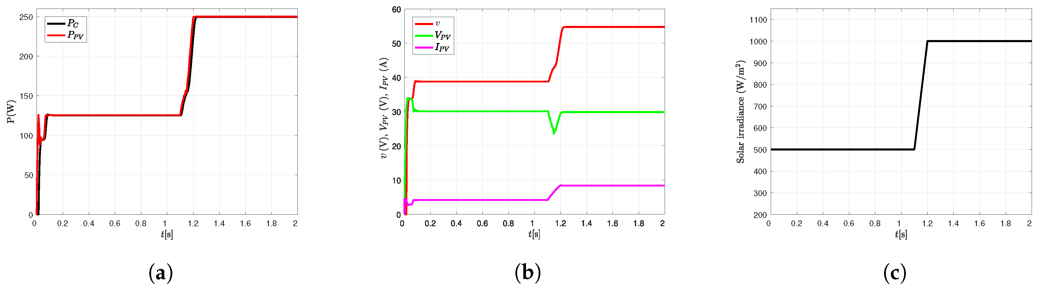
Case 1. At 1.1 s, the solar irradiance is increased from 500 W/m
to 1000 W/m
within a time interval of 0.1 s. A constant temperature of 25
C is considered (see
Figure 7c).
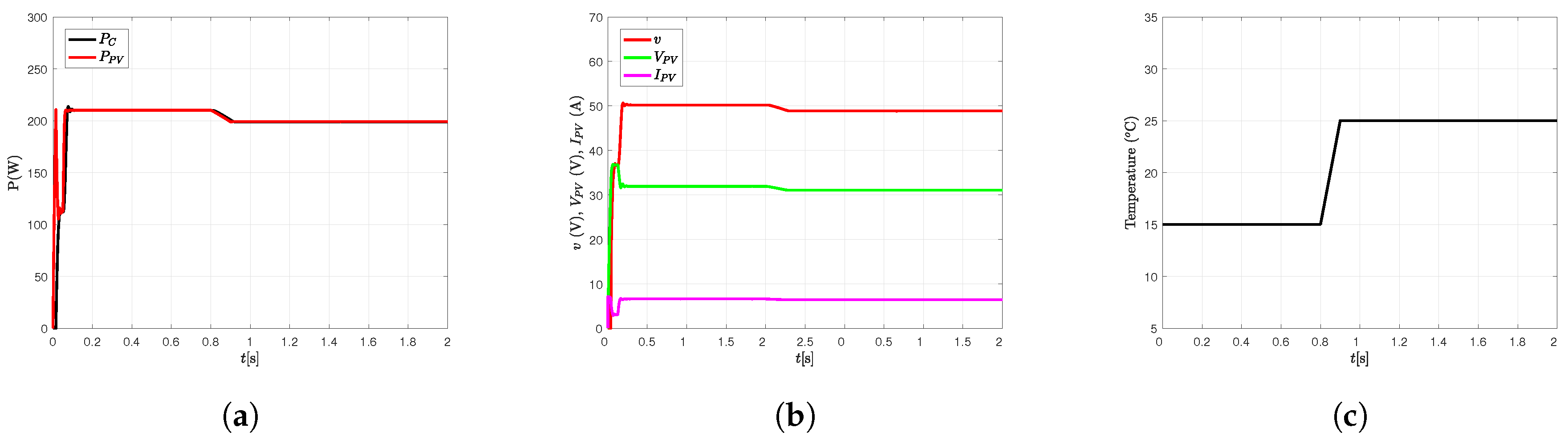
Case 2. At 0.8 s, the temperature is increased from 15
C to 25
C within a time interval of 0.1 s. A constant solar irradiance of 800 W/m
is considered (see
Figure 8c).
Case 3. Considering a constant temperature of 25
C, at 0.6 s, the solar irradiance is decreased from 1000 W/m
to 500 W/m
within a time interval of 0.5 s. Then, at 1.2 s, the solar irradiance is increased from 500 W/m
to 1000 W/m
within a time interval of 0.5 s. In a different time instant (at 2 s), the temperature increases from 25
C to 40
C within a time interval of 0.1 s (see
Figure 9c).
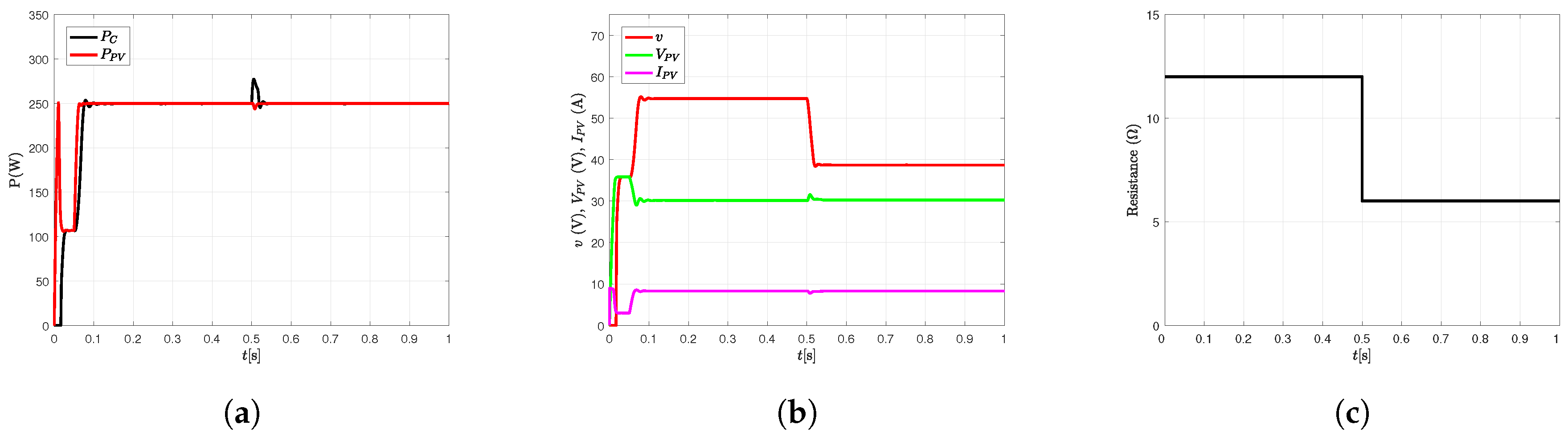
Case 4. A solar irradiance of 1000 W/m
and a temperature of 25
C are kept constant while the load instantly decreases from 12
to 6
at 0.5 s (see
Figure 10c).
In the first three cases, a constant load of 12 is considered.
Note that the proposed time scales are short (tests were performed within time intervals less than 3 s). This aims at demonstrating the strength of the proposed approach for the MPPT, i.e., to evaluate the performance of the flatness-based control law against sudden variations of weather conditions. Clearly, if the controller is efficient in tracking the MPP in spite of the abrupt changes considered in the study cases described above, it will also have a satisfactory performance under realistic operating conditions involving smoother variations of solar irradiance and of temperature, occurring within longer time intervals.
Figure 7,
Figure 8,
Figure 9 and
Figure 10 illustrate the performance of the proposed control approach under the conditions stated above.
Table 3 presents the theoretical maximum power for the different values of temperature and solar irradiance considered in the four study cases. It is important to mention that, theoretically, load variations do not affect the maximum power.
The trajectories generated under the conditions described in
Case 1 are depicted in
Figure 7. The output power of the Boost converter and the power delivered by the PV panel are shown in
Figure 7a. The output voltage of the converter and the current and voltage of the PV panel are presented in
Figure 7b.
Figure 7c shows the variation of the solar irradiance. Note that the theoretical values of the maximum power for a constant temperature of 25
C are reached: 125 W for a solar irradiance of 500 W/m
, and 250 W for 1000 W/m
. Observe that, as expected, during the time period in which the solar irradiance increase takes place (from 1.1 s to 1.2 s), an increment of the current of the PV panel occurs. However, the voltage
is kept at a constant value (except for the variation observed within the time lapse in which the solar irradiance variation occurs).
The system response obtained by considering the conditions stated in
Case 2 is illustrated in
Figure 8.
Figure 8a depicts the Boost converter output power as well as the power delivered by the PV panel.
Figure 8b shows the output voltage of the converter and the current and voltage provided by the PV panel. The variation of temperature is presented in
Figure 8c. In this case, an increase of temperature occurs from 0.8 s to 0.9 s. In this period of time, the power values are decreased from 210 W/m
to 200 W/m
. These values are in accordance with the theoretical maximum power that can be achieved (see
Table 3). As expected, the current of the PV module remains constant and the value of
decreases.
The controller performance under the conditions described in
Case 3 is illustrated in
Figure 9.
Figure 9a presents the output power of the Boost converter and the power delivered by the PV panel.
Figure 9b shows the trajectories of the converter output voltage as well as the voltage and current values delivered by the PV panel.
Figure 9c illustrates the solar irradiance and temperature variations. It is obvious that when a decrease of solar irradiance occurs, the power provided by the PV panel
and the current
also decrease meanwhile the voltage
does not vary significantly. Conversely, when solar irradiance increases, the power provided by the PV panel
and the current
are also incremented meanwhile the voltage
undergoes variations but after a short period of time it reaches the previous value again. The temperature increase leads to a slight reduction of the voltage
and a decrease of the power
meanwhile the current
remains almost unchanged. Notice that in all cases the theoretical maximum value of the power provided by the PV panel is achieved (see
Table 3).
The controller performance under the conditions described in
Case 4 is illustrated in
Figure 10.
Figure 10a shows the output power of the Boost converter and the power delivered by the PV panel.
Figure 10b shows the trajectories of the converter output voltage as well as the voltage and current values delivered by the PV panel.
Figure 10c illustrates the load variation. Note that the load is diminished at 0.5 s leading to minor variations of the signals coming from the PV panel
,
, and
. However, the output voltage of the Boost converter
v is significantly decreased. It is noteworthy that variations of the load do not prevent the proposed algorithm from successfully tracking the maximum power.
Simulation results highlight the performance of the proposed control approach. Case 1 is defined to demonstrate the robustness of the control law against solar irradiance abrupt changes; Case 2 aims to show the controller performance under a sudden variation of temperature; Case 3 allows evaluating the performance of the controller under abrupt variations of solar irradiance and temperature; finally, Case 4 considers the transit from a lightly loaded system to a heavily loaded one.
Simulation results show that the proposed control scheme is robust against variations of external conditions and that the corresponding values of maximum power are reached in all cases. From
Figure 7,
Figure 8,
Figure 9 and
Figure 10, it can be noticed that the control action takes about 0.1 s to be reflected in the system trajectories and that the system reaches the steady state in a very short period of time regardless the variation of weather conditions and load. This stabilization time can be considered acceptable since most of the PV applications do not require a faster response.
As can be seen, the sudden variations of temperature, solar irradiance and load do not degrade the performance of the flatness-based controller. It can be concluded that the flatness-based controller is effective in maintaining the output power of the PV panel at the corresponding optimum values. Furthermore, it is robust against variations of external conditions and operates under low or high temperatures.
Comparative Analysis
In order to determine the benefits that the proposed control scheme offers in contrast to the most popular MPPT techniques: Perturb and Observe (P&O) and Incremental Conductance (IncCond), numerical simulations were performed. Under the conditions stated in
Case 3, the conventional P&O method (see for instance [
12]) and the IncCond with integral regulator (IncCond+IR) algorithm proposed in [
39] were evaluated.
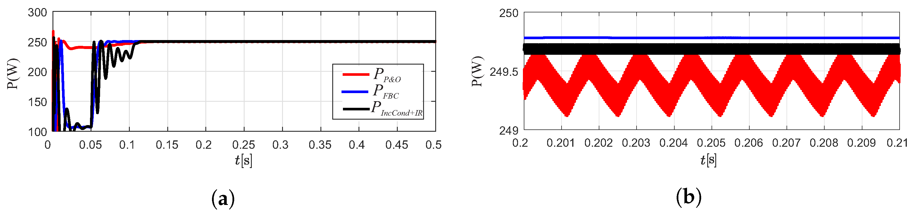
Figure 11 shows the performance of these three techniques;
corresponds to the power obtained with the P&O method,
is the power obtained with the flatness-based control technique proposed in this paper, and
is the power obtained with the IncCond+IR algorithm.
Note that within the time interval where the solar irradiance increase occurs (between 1.2 s and 1.7 s), the response produced with the flatness-based approach differs from the ones produced with the other techniques. However, the theoretical power is reached when the solar irradiance is set at 1000 W/m.
At first glance, it might seem that the three methods have almost the same performance, however, a zoom of
Figure 11 shows that, although the time to reach the MPP is almost equal (about 0.13 s), the response obtained with the IncCond+IR method exhibits oscillations of significant magnitude before reaching the MPP (see
Figure 12a), and that, as expected, the response produced with the P&O technique presents small amplitude oscillations around the MPP (see
Figure 12b).
In view of the simulation results, it can be concluded that one important advantage of the proposed approach is that less oscillations are produced before reaching the MPP compared to the IncCond+IR method. Furthermore, the flatness-based method does not give rise to oscillations around the MPP, like the ones observed for the P&O technique.
Another disadvantage of the P&O technique is that its accuracy depends on the perturbation size: if it is small, the method takes more time to reach the MPP, if it is big, the amplitude of the oscillations around the MPP increases [
26]. This does not occur with the proposed flatness-based method.
5. Experimental Results
Experimental results obtained with a PV panel Virtus II model JC250M-24/Bb show the performance of the flatness-based controller under realistic scenarios. For the implementation of this MPPT controller, a Boost power converter is designed to operate in continuous mode at a switching frequency of 45 kHz; the parameter values used in the experimental set up are shown in
Table 2.
The MPPT flatness-based control algorithm was implemented with the Simulink Real-Time
® software (R2015a, The MathWorks, Inc, Natick, MA, USA) using a Humusoft
® MF 624 multifunction I/O card (MF624, Humusoft Ltd., Prague, Czechia) that is installed on a computer with an Intel
® Core
TM processor (i7-2600, 3.40 GHz, Intel, Santa Clara, CA, USA) and 8GB RAM memory (DDR3 1333 MHz, Hynix, Incheon, Korea). The complete scheme operates at a fixed sampling frequency of 10 kHz. A PWM generator set to a frequency of 45 kHz is employed. Four analog inputs are used to sense the current
and voltage
of the PV panel, the output voltage of the converter
v, and the current through the load resistor
, which allows monitoring possible variations of the load. The control system can be described as follows. The input signals
and
are acquired by sensors S22P (current) and AMC1100 (voltage) respectively. The average control signal
adjusts the duty cycle of the PWM generator which activates the MOSFET 19NF20 through the optocoupler circuit IX3180. The auxiliary input
defined in Equation (
19) is generated with the use of the reference signal
(derived from the output voltage reference) and the flat output
F. The Vantage Pro2
weather station is used to measure solar radiation; it is remotely connected with an indicator console. The experimental configuration diagram, the nominal values of the components, and the information of electronic devices and sensors are shown in
Figure 13.
It is important to mention that the true MPP is unknown during a real-time test under natural sunlight. This is because the temperature cannot be accurately measured since PV panels have a multicell distribution and an insulated laminated structure [
40].
During the development of experiments, temperature differences of more than 5 C were found in different sections of the PV panel. Higher temperatures were identified near to the edges of the PV panel due to the heating generated by its laminated structure. To cope with this, approximate values of the panel temperature were calculated from the average of the measured temperatures. Based on these values, the corresponding values of the theoretical maximum power were obtained.
The first experimental test was carried out when a solar irradiance of 510 W/m
was measured and an average temperature of 35
C was calculated.
Figure 14 shows the closed-loop response of the system under these conditions.
Figure 14a corresponds to the experimental result and
Figure 14b to the simulation response.
The second test was conducted under a solar irradiance of 900 W/m
and an average temperature of 45
C. The system response is shown in
Figure 15.
Figure 15a corresponds to the experimental result and
Figure 15b to the simulation response.
Notice that, in simulation, the theoretical maximum powers are reached (118 W for the first case, 203 W for the second one, see
Table 3), meanwhile the powers obtained with the experimental tests are below these values (around 110 W for the first case, around 190 W for the second one). As explained before, these differences between the power values are due to the fact that it is impossible to estimate precisely the true MPP value based on the weather conditions because of the complexity of module lamination and measurement accuracy [
40]. Besides, there are power losses in the connection cable between the photovoltaic module and the converter that should be considered. In [
41], it is shown that the theoretical MPP values can be either higher or lower than the practical measured tracking values. Despite this, from
Figure 14a and
Figure 15a it can be inferred that the flatness-based controller allows delivering all the available power to the load.

 ,
, 


