Article

Integrated Techno-Economic Power System Planning of Transmission and Distribution Grids

1
Centre for Sustainable Energy Systems, Flensburg University of Applied Sciences, Kanzleistraße 91-93, 24943 Flensburg, Germany
2
Reiner Lemoine Institute, Rudower Chaussee 12, 12489 Berlin, Germany
3
Centre for Sustainable Energy Systems, Europa-Universität Flensburg, Auf dem Campus 1, 24943 Flensburg, Germany
4
Institute for Intelligent Cooperative Systems, Otto-von-Guericke-University Magdeburg, Postfach 4120, 39016 Magdeburg, Germany
5
DLR Institute of Networked Energy Systems, Carl-von-Ossietzky-Str. 15, 26129 Oldenburg, Germany
*
Author to whom correspondence should be addressed.
Energies 2019, 12(11), 2091; https://doi.org/10.3390/en12112091
Submission received: 19 March 2019 / Revised: 9 May 2019 / Accepted: 26 May 2019 / Published: 31 May 2019
(This article belongs to the Section F: Electrical Engineering)

Abstract

:
The energy transition towards renewable and more distributed power production triggers the need for grid and storage expansion on all voltage levels. Today’s power system planning focuses on certain voltage levels or spatial resolutions. In this work we present an open source software tool eGo which is able to optimize grid and storage expansion throughout all voltage levels in a developed top-down approach. Operation and investment costs are minimized by applying a multi-period linear optimal power flow considering the grid infrastructure of the extra-high and high-voltage (380 to 110 kV) level. Hence, the common differentiation of transmission and distribution grid is partly dissolved, integrating the high-voltage level into the optimization problem. Consecutively, optimized curtailment and storage units are allocated in the medium voltage grid in order to lower medium and low voltage grid expansion needs, that are consequently determined. Here, heuristic optimization methods using the non-linear power flow were developed. Applying the tool on future scenarios we derived cost-efficient grid and storage expansion for all voltage levels in Germany. Due to the integrated approach, storage expansion and curtailment can significantly lower grid expansion costs in medium and low voltage grids and at the same time serve the optimal functioning of the overall system. Nevertheless, the cost-reducing effect for the whole of Germany was marginal. Instead, the consideration of realistic, spatially differentiated time series led to substantial overall savings.

1. Introduction

Historically in Germany, electric energy was supplied by large conventional power plants in the transmission grid to consumers mainly connected to the distribution grid. Distribution grids were therefore dimensioned to ensure power supply in extreme load cases. In this context, the clear division of transmission and distribution operation and planning is reasonable.
In the year 2000, the German Renewable Energy Act was introduced in order to reduce greenhouse gas emissions, leading to a strong expansion of renewable energy (RE) systems, which is expected to be continued in the future. By 2050 at least 80% of Germany’s electricity demand is supposed to be supplied by RE production [1]. Due to their relatively small nominal power these power plants are mainly connected to the distribution grid (e.g., [2,3]). This substantial transition of energy supply structure leads to more diverse power flow characteristics (e.g., [4,5,6]). In simple terms, unidirectional flow patterns are shifted to bidirectional ones. Distribution grids not only distribute but also supply power changing their behavior with respect to the mostly weather-dependent renewable power production. The increase of complex interdependencies between the different voltage levels calls for research on integrative transmission and distribution grid planning (see also [6]).
Furthermore, the described energy transition most likely leads to substantial grid and storage expansion needs in the German power system (e.g., [2,3,7,8,9,10]). For society it is of interest to find economically efficient solutions. In this spirit, a combined economic optimization of grid and storage expansion considering technical constraints seems to be a worthwhile task.
On the one hand, the need for combined optimization of grid and storage expansion and on the other hand the spatially detailed integrative consideration of all voltage levels motivate this work and lead to the following research questions:
  • How is it possible to integrate transmission and distribution grid planning?
  • Is it (systematically) cost-efficient to align distribution grid planning with the overall systematic optimization of power plant dispatch, grid and storage expansion?
This work explicitly uses and creates open data and open source tools. The underlying paradigm is motivated by multiple considerations. Due to the lack of available grid data, open data methods enable and enhance independent and diversified research. Additionally, the good scientific practice aims to create reproducible methods and results. Last but not least, the energy transition displays a fundamental societal effort which may be better addressed in a transparent way to raise public acceptance for scientifically reasonable changes. Recently these aspects have been addressed more often in energy research gaining greater relevance (e.g., [11,12,13,14,15]).
The following Section 2 provides an overview of the state of the art of transmission and distribution grid planning. Here, we primarily focus on the research and best-practice principles which are conducted and applied by transmission and distribution grid operators. Thereafter, a novel approach of integrated transmission and distribution grid planning is presented (Section 3). First, a brief introduction to the underlying grid model is provided. Second, the methods used to optimize grid and storage expansion on the extra high (EHV) and high voltage (HV) level are described. Third, the interface to the medium (MV) and low voltage (LV) level is characterized. Lastly, the grid expansion, storage and curtailment distribution methods on these lower distribution grid levels are specified. Based on this we present, discuss and critically address our results for a mid-term and a long-term future scenario (Section 4 and Section 5) before we conclude our findings in the last section.

2. State of the Art

The following two subsections set the basis for the further understanding of our novel applied research approach by presenting an overview of today’s transmission and distribution grid planning. The aim is to outline the general grid planning from a German grid operators’ perspective. We therefore mainly focus on planning principles applied in practice rather than the state of theoretical research.

2.1. Transmission Grid Planning

Currently, the German power transmission grid is maintained by four transmission system operators (TSO) and future developments are documented and adapted continuously in the grid development plan [16]. To create those grid development plans, TSO use energy system models to represent the interaction of various components like grid, generation, demand, and markets in an interconnected energy system. In this context various opportunities and requirements in future energy system scenarios are modelled with the help of computer simulations.
The methodological approach of the official grid development plans can be summarized by the following heuristic. At first, TSOs apply information about the future load and generation development estimating their technological, temporal and spatial characteristics. These values are mapped to the nodes of the transmission grid via various approaches and data sets. A market simulation defines the dispatch of the power plants matching the assumed demand. At last, power flow simulations are executed which may result in critical line loads. In this case, these critical line loads are eliminated by iteratively applying grid optimization, strengthening and finally expansion measures (prioritization of measures in Germany referred to as NOVA-principle) [16]. Furthermore, the TSOs are not only responsible for the security of supply during normal operation but also in case of contingencies. Therefore, (n-1) contingency analyses are performed to assess the capability of the grid to sustain various combinations of power grid component failures [17]. Consequently, reserve capacity is provided to fulfill the so-called (n-1) security. The (n-1) security is a common principle to ensure a power supply even if a single component of the system fails [18].
Appropriate models of the transmission grid are often used to analyze impacts due to the integration of a higher amount of RE resources [19] and coupled with the energy dispatch [20]. Depending on their focus, transmission grid models vary in their type of power flow simulation, the level of detail regarding the grid, spatial and temporal resolution as well as the extension of the grid and management of bottlenecks. Especially power flow simulations apply several approaches such as DC, PTDF, AC or NTC [21], which lead to different degrees of accuracy and computational effort. The trade-off between accuracy and computational burden leads to a wide range of existing approaches to model the transmission grid. Besides the power flow simulations, there are different methods to represent power flow monitoring devices like phase-shifting transformers or high-voltage DC transmission links which may be used more often in the future grid [22]. The results of power flow simulations in combination with a grid model help to identify bottlenecks of the grid and to prevent them with an adapted energy redispatch [23]. If this prevention is impossible, models enable to evaluate possible actions such as reinforcing or extending the transmission grid [24].

2.2. Distribution Grid planning

Distribution grid operators are, just as transmission grid operators, obliged by the German Energy Act [25] to guarantee a safe and reliable electricity supply at a certain quality. To ensure fulfillment of these objectives, distribution grid planning focuses on compliance with allowed limits for thermal loading of network equipment and voltage deviations.
Allowed voltage deviations of the supply voltage are specified in DIN EN 50160 [26]. According to [26], voltage deviations under normal conditions in MV and LV grids must be kept below 10% relative to the nominal voltage. Regarding supply voltage in HV grids, [26] does not specify fixed limits but states that it must be defined in coordination with each grid user as the number of grid users connected to the HV grid is limited, and supply is based on individual contracts. Furthermore, guidelines [27,28] define allowed voltage deviations caused by distributed generators (DG) in MV and LV grids with respect to voltage deviations without DG feed-in of 2% and 3%, respectively.
Thermal loadings of network equipment are among others defined in DIN EN 60076 [29] and DIN VDE 0276-603 [30]. In addition, load factors are defined by the distribution system operators (DSOs) that further limit allowed thermal loading under normal conditions to ensure reserve capacity for (n-1) security. Although being more relevant in the transmission grid, the (n-1) principle also applies for generators connected to the HV grid and consumers connected to the HV and MV grid; it does not usually apply for consumers connected to the LV grid nor for DG in the MV and LV grid [2,3,31].
In traditional grid planning, overloading and voltage issues are mostly resolved by grid expansion measures. If possible, a modification of the switching state or the control voltage are as well deployed, though less commonly. Although there are different guidelines for distribution grid planning, every DSO defines their own principles adjusted to their historical and operational conditions. Economic efficiency is motivated to be considered for the applied measures by regulation [32]. Therefore, usually a general cost efficiency paradigm such as the NOVA-principle is used not only in transmission grid planning (see also previous section). Commonly, grid planning is conducted separately for the different voltage levels. Prevailing measures are replacement of equipment by equipment with a higher capacity or reinforcement through parallel equipment. These measures increase the thermal capacity and may have a positive impact on voltage stability by decreasing grid impedance. Another option is adapting grid topology e.g., by adding a new substation. [2,3,31,33]
Necessary grid expansion measures are usually identified for two extreme loading cases with fixed simultaneities for loads and generators—the heavy load flow (HLF) and the reverse power flow (RPF). The HLF is characterized by maximum demand and zero or small feed-in by generators in the grid. The demand is in that case supplied by the upstream grids. The RPF is characterized by high feed-in of generators and small demand. Excess power is fed to the higher voltage grid. The RPF becomes increasingly relevant as capacity of DG increases [3,31,33]. It is deliberately not defined by maximum feed-in as a targeted reduction of feed-in of wind and solar generators is already an applied planning principle [2]. However, the exact definition of simultaneities for both design cases usually depends on broad assumptions by the grid operator.
In addition to feed-in management, further innovative options supplementing conventional grid reinforcement to solve new challenges arising from the transformation of the energy system have become available [34]. These supplementary options can be distinguished between innovative grid operation concepts such as demand response and reactive power management on the one hand and on the other hand innovative network equipment such as on load tap changers and battery storage units [35]. For an holistic assessment incorporating all these options to find the most efficient combination, time-dependent variables such as the amount of curtailed energy, grid losses and provided reactive energy have to be considered [36]. In transmission grid planning analyses based on feed-in and demand, time series are already state-of-the-art [37] and could consequently be applied in distribution grid planning.
Furthermore, a number of these novel options as well as the transformation of the generation landscape and the planned electrification of the heat and mobility sectors will impact dependencies and simultaneities on the demand and generation side, making simplified worst-case assumptions based on sweeping standardized factors less precise and thus leading to an over- or underdimensioning of the grid [35]. Numerous studies have therefore analysed and reviewed new innovative grid planning methods and design cases [35,36,38,39,40], though these are not widely applied by DSOs.

3. Methods

The software tool eGo aims at optimizing the electrical grid and storage devices throughout all voltage levels. This is achieved by a top-down approach: First, the integrated EHV and HV grid is optimized with the tool eTraGo (Section 3.2). Subsequently, a selection of MV (and subordinate LV) grids are simulated and optimized with the tool eDisGo (Section 3.3.3). This approach requires an interface which transforms the top-level optimization results into input data for the lower grid levels (Section 3.3.1). Moreover, the selection of MV grids was systematically determined and used for generalization (Section 3.3.2). All of these methods are based on a data model that is mainly described and partly validated in previous works [14,41,42]. Recently, [6,43] used that same data basis. For the sake of integrity it is briefly presented in Section 3.1.

3.1. Data Model

The investigation of the cross-voltage-level electrical power grid with the developed models eTraGo [44] for EHV and HV (≥110 kV), eDisGo [45] for MV and LV and eGo [46] which joins both models (see also Section 3.2 and Section 3.3 below) is based on a coherent, fundamental data basis. This data basis relies on open data sources such as OpenStreetMap (OSM) [47] and is open and freely available on the complementary developed OpenEnergy-Platform (OEP) [48] and OpenEnergy-Database (oedb) [49]. In this work, the data version v0.4.5 was consistently used.
Beginning from the fundamental data basis, a sequential processing of raw data is conducted by the software tool data processing [50] and creates the structured input format for the German EHV and HV power grids and provides a pre-processed input for the tool Ding0 [51] which creates synthetic MV and LV grid models considering DG and demand.
The two resulting input data models are at an hourly and geographically high resolution. The methods and assumptions of the allocation of electricity consumption and power generation capacities in a high spatial resolution for both data sets are described in a previous article [41]. The developed EHV/HV grid topology model for Germany is based on OSM data and is created with the heuristic abstraction tool osmTGmod [52]. By revising the tool, the 110 kV grid was integrated into the grid topology [14]. All existing border crossing power lines of the neighbouring countries are connected to the detailed German grid model with respect to their voltage level. MV and LV grid topologies are, as mentioned, synthesized using the tool Ding0 taking into account local characteristics, such as demography and land use, and former planning principles. MV grid topologies are modeled as open half-rings. LV grids are modeled as radial networks using reference grids from [53,54]. The in-depth scientific explanations of the EHV/HV power grids [14] and the MV grid models [42] specify the further methods and assumptions leading to suitable data sets for the power grid planning tools. In comparison to standard transmission grid planning, the voltage level of 110 kV is included in the top level optimization of eTraGo.
For the representation of the weather dependent power generation, the feedinlib [55] is used. The feedinlib is a tool that generates feed-in time series of solar and wind generators from given weather and generator data. Here, coastDat-2 [56,57] weather data of the year 2011 with a spatial resolution of 0.22 degrees is applied. Due to the complexity and missing detailed information, generic solar and offshore wind power plants are used. In contrast, onshore wind power plants are differentiated by seven power classes characterizing typical wind onshore turbines in terms of installed capacity and installation site (regarding the register of RE plants of the BNetzA [58]).
Three scenarios are defined representing the German power system of 2015 (Status Quo) and of the future (NEP 2035 [7] and eGo 100 [15,59]). In this work, particularly the two future scenarios are utilized. The scenarios mainly differ by the share of RE sources in installed capacity (for Germany: Status Quo: 47%, NEP 2035: 70% and eGo 100: 100%; cf. [14]). In Figure 1 the installed generation capacities are displayed for each scenario and technology. Note that, in the eGo 100 scenario a few gas fired power plants in the neighboring countries were tolerated with respect to [60] (cf. [14]). The net electricity consumption, the annual peak load and weather year are assumed to be the same in all scenarios. The EHV/HV and MV/LV grids represent grids that are stable in the Status Quo scenario and are the basis of the optimization of the grid topologies in the two future scenarios.
The resulting data sets are considerably large and complex. For instance the eGo 100 scenario contains an EHV/HV grid with 11,305 buses, 19,169 power lines, 526 transformer, 3597 aggregated loads and 19,022 aggregated generators (differentiated by technology as displayed in Figure 1) including hourly generation and demand time series for the entire scenario year. In Figure 2a the EHV/HV grid topology (without generation and demand) is displayed. Regarding the underlying voltage levels there are a total of 3591 MV grid districts. These include 215 urban grid districts that are not further considered as it is assumed that grid expansion needs due to an increase of DG capacity are neglectable. This results in 3376 synthetic MV grids which include all single generators, loads, HV-MV substations and MV-LV substations of the voltage level down to 0.4 kV. It is assumed that each MV distribution grid is connected to the HV level via transformers at only one substation. This assumption reflects the status quo in Germany and implies that during normal (n-0) operation, tie points between neighboring MV grids are operated as open switches [3,61,62,63]. Possible changes of the HV feeding situation by closing normally open tie switches are not considered. Consequently, the HV-MV substations are suitable as consistent and exclusive interfaces to the HV level. One of these MV grids is topologically presented in Figure 2b.

3.2. Optimization of Extra-High and High Voltage Levels

Addressing the high complexity of the data model, we used certain reduction methods which abstract the temporal and spatial resolution.
The spatial resolution was reduced by adapting a reduction method described in [9]. Therefore, the original number of buses was decreased by applying a k-means clustering algorithm using Python’s scikit learn package (cf. [64]). The weighted squared euclidean distances of each k centroid to its clustered members are minimized by performing the following iterative expectation–maximization (E–M) algorithm (see also exemplary visualization in Figure 3).
  • Guess k cluster centers
  • Repeat until converged
    (a)
    E-Step: assign points to the nearest cluster center
    (b)
    M-Step: set the cluster centers to the mean [65]
The weight of each original bus is relative to its today’s (referring to the status quo scenario) load and conventional generation capacity. In this work we chose a k of 300. Thus the 11,305 buses (consisting of 7108 joints and 4197 buses being connected to load, generation and/or transformer(s)) are reduced to this value. The topological difference before and after clustering can be observed by comparing the original complexity in Figure 2a with the final one in Figures 10 and 11. For comparison of the results of several optimization runs, the abstracted topology was reproduced by using the same once randomly generated initial k positions for the k-means algorithm. This method implies that beforehand the 220 and 110 kV buses and lines are upgraded to a nominal voltage of 380 kV. Hence, according to Equation (1) the lines’ (Index l) reactances (x) and resistances (r) were changed considering their original nominal voltage ( v _ n o m l , in kV). Consequently, all transformers are modelled as lines.
r , x l , 380 = r , x l · 380 v _ n o m l 2 , l L
All lines between two clusters are represented as one. The nominal capacities and the admittances of the original lines were summed up accordingly.
The generators and storage units at the buses are aggregated with respect to the carrier type. Considering weather-dependent resources (i.e., wind and solar) which differ from one weather cell to another, the power plants normalized maximal possible power outputs are weighted by their capacities within one carrier type. In the case of storage units, the aggregation differentiates additionally according to the power-to-energy (P-E) ratio.
The temporal resolution can be reduced by various clustering methods. Coming to inter-temporal restrictions which the dispatch of storage units imply, many of those methods are limited in their performance. In this work, we chose a simple solution which periodically leaves out snapshots (cf. [9]). Particularly, we considered only every fifth hour. This reduces the run-time of eTraGo substantially and also implies significant run-time savings for the following processes in eDisGo (see Section 3.3.3).
The reduced data set was subject to a linear optimal power flow method (LOPF) [66]. Optimization variables are grid ( F ) and storage investments ( H n , s ) as well as the dispatch variables of generators ( g n , r , t ) and storage units ( h n , s , t ) (see Equation (2)). The indices , n , r , s , t label branches, buses, generators, storage units and the hour of the year. The dispatch optimization considers the marginal costs (EUR/MWh) for generators ( o n , r ) and storage units ( o n , s ). Due to the applied temporal complexity reduction, each snapshot is weighted as w t = 5 . The specific capital costs (EUR/MW) for each branch (power line, link or transformer) and each storage unit s are defined by c and c n , s .
min F , H n , s g n , r , t , h n , s , t c · F + n , r , t w t · o n , r · g n , r , t + n , s c n , s · H n , s + n , s , t w t · o n , s · [ h n , s , t ] +
The assumptions on the investment costs can be observed in Table 1. Considering technological progress, storage units are assumed to have smaller investment costs for the eGo 100 scenario [67]. In the case of the other components, no differentiation between scenarios was taken into account. The values for the AC power lines shown in Table 1 are based on the assumption that additional systems can be attached to the existing poles. In contrast, assumptions for a complete reconstruction are according to [3] for the HV level and [7] for the highest voltage level approximately four times higher. As a cautious premise we therefore took into account four times higher costs since in most cases a new construction would be necessary. Lines and transformers are assumed to have lifetimes of 40 years whereas storage units last 25 years. Additionally, assuming an interest rate of 5%, the overnight investment costs were annualized. The marginal costs of the generators for the different scenarios are taken from [14].
The modelling of storage units is precisely based on a previous work [43] in which the corresponding assumptions and methods are described in detail. Two different storage technologies were considered, potentially providing short-term and long-term flexibility to a future electricity system. Battery storage units could be built at every node and operate on an hourly scale being able to store and provide energy for six hours at full capacity [43]. In contrast, the hydrogen storage units have a much higher P-E ratio of 1 / 168 and could only be built at certain buses where the potential of natural salt caverns is given [43]. Moreover, all lines, DC links and transformers were assumed to be extendable. The grid expansion was limited such that each line could be extended by a maximum of four times its original capacity. Avoiding a mixed integer linear problem, grid and storage expansion are optimized continuously as stated in Equation (2).
In the LOPF, the maximal possible power flow over a line or transformer is constrained by its nominal thermal limit capacity. Concerning n-1 security it was assumed that all grid components being operated at 380 and 220 kV grid can be loaded at a maximum of 70% of their nominal capacity [13]. Presuming a less redundant HV grid with an average of two parallel systems (according to the osmTGmod data model the average number of parallel power line systems is 1.9), the 110 kV components can be used at a maximum of 50%. Regarding the cross-border power lines, we reduced the n-0 thermal capacities and instead assumed net transfer capacities from 2015 [68] as a status quo base. By this, we aim to avoid an overestimation of the possibility to trade electricity from one market region to another.
The LOPF led to results concerning active power flows and dispatches. In the interest of simulating reactive power flows, it was followed by a non-linear Newton-Raphson power flow algorithm (PF). As a prerequisite, another LOPF was realized which uses updated reactances of the expanded lines (calculated according to Equation (3)). Here s _ n o m l and s _ n o m _ o p t l represent the nominal capacity of a line before and after optimization. Therefore, it is assumed that the additional line capacity is installed as a parallel circuit to the original one. Thus, the second LOPF re-optimizes the dispatch considering the updated reactances within the linearised AC power flow equations.
x _ o p t l = x l · s _ n o m l s _ n o m _ o p t l , l L
The optimized dispatch of this second LOPF is used for all generators and storage units as p s e t , which has to be met within the PF problem. All aggregated generators are modelled as PV generator since a resolution of k = 300 leads to sufficient aggregate sizes. Consequently, the reactive power dispatch will be a variable to be determined by the PF. The reactive power will be produced locally where it is demanded. The reactive behavior of the grid components and the aggregated loads is considered. The aggregated loads are assumed to have a power factor cos ϕ of 0.95 (inductive) [14,69]. The bus with the largest annual dispatch in the LOPF is defined as the slack bus for the PF [14,70].

3.3. Incorporation of the Medium and Low Voltage Levels

This section describes (1) the design of the interface between the HV and MV level, (2) the complexity reduction and generalization on MV and LV grid levels and (3) the simulation and optimization of the MV and LV grids themselves.

3.3.1. Interface Design

The central reference points for the interface are HV-MV substations. In open_eGo, they are identified throughout the above described data processing [41,42]. HV-MV substations represent the highest resolution for the top-level optimization (generators and loads are aggregated at this level). At the same time, they serve as slack buses for the subordinate MV grids.
As described above, a clustering method is applied to the integrated EHV and HV grid in order to reduce its spatial complexity. For this reason, the first step of the interface consists of distributing the optimization results back to the original HV-MV substations, a process which is called disaggregation.
During disaggregation, the optimization results obtained for the clustered optimization problem are distributed uniformly using specific weights, depending on which type of component the results where computed for. More specifically, for each generator representing a cluster, its active and reactive power time series are distributed to the generators the cluster represents, while for storage units, the state of charge and the optimized installed capacity are also distributed. Note though, that the latter value in particular is not time dependent. As stated above, the formulas used to distribute values computed for a cluster differ, depending on which type of component they are generated for. These distribution strategies are explained in the following, starting with how storage capacities are distributed.
Equation (4) contains H, the optimized storage capacity, and h ^ , the upper bound on how much storage capacity is allowed to be installed as part of the investment. The other auxiliary symbols used in Equation (4) are the cluster index k and the set of indexes of storage units of a certain type represented by the cluster k, denoted by N k . This means, that storage capacity is distributed via a weighted average where the weight is determined by the fraction that the upper bound on the investment on a storage’s capacity contributes to the sum of all such upper bounds. In Figure 4 this disaggregation is exemplarily visualized for one aggregated battery storage unit.
H s = H k · h ^ k s N k h ^ s
The distribution of state of charge, denoted by s o c , and power output, denoted by h, is governed by Equations (5) and (6), which are similar to Equation (4), except that they have to take into account the current snapshot t, as the values they are distributing are time dependent.
s o c s , t = s o c k , t · H s s N k H s
h s , t = h k , t · h ¯ s , t s N k h ¯ s , t
Again, the values are distributed as weighted averages, except that the weights are determined differently now. For the state of charge, the weight is determined by the fraction the nominal capacity H of a storage unit contributes to the sum of all nominal capacities of storage units of a certain type represented by a cluster, whereas for power output, denoted by h ¯ , the weights are determined by the fraction the maximum possible power output of a component at a certain snapshot contributes to the total maximum possible power output of components of the same type at a certain snapshot. Note that Equation (6) holds for storage units as well as for generators. Furthermore, bear in mind that all unexplained symbols in Equations (5) and (6) have the same meaning as in Equation (4).
Subsequent to the disaggregation of eTraGo’s results, the input parameters are calculated for the selected MV grids. Here, the crucial parameter is the generator dispatch (active and reactive power). At the interface level, the generator dispatch is differentiated by energy carrier (e.g., wind and solar) and weather cell and it is normalized with the installed capacities respectively. In eDisGo, these normalized time-series are then allocated to the individual generators of the corresponding MV grid. In order to limit reactive power flows and thus, cap the additional burden on MV grids, the reactive power dispatch of wind and solar generators is limited to cos ϕ = 0.9 .
With regard to fluctuating generators (wind and solar), the dispatch comprises the uncurtailed potential only. In addition to the potential, an absolute amount of curtailment is calculated per energy carrier and weather cell. This approach allows certain degrees of freedom when allocating the absolute amount of curtailed energy to the individual generators in eDisGo (cf. Section 3.3.3).
In eTraGo, the installation of storage units is an essential parameter of the investment optimization. It is important to note that the intended purpose of storage units is not only limited to a temporal balance of energy. They can be furthermore used in a grid-supportive manner. In order to make this grid-supportive characteristic available also to MV grids, eDisGo optimizes the spatial distribution of the installed batteries within each MV grid. Thereby, the active and reactive dispatch of storage units becomes another crucial parameter of the interface. In addition, here it should be noted that the dispatch is already optimized by eTraGo. eDisGo only optimizes the spatial distribution of the already determined dispatch.

3.3.2. Complexity Reduction

As mentioned in Section 3.2, the temporal resolution was reduced by only considering every fifth hour. Furthermore, a spatial clustering was applied to the original HV-EHV network. In order to achieve acceptable computation times, another spatial reduction was necessary with regard to the MV grids. Simulating the total number of over 3000 MV grids was beyond the scope of this study. Instead, the objective here was to estimate the total costs of grid expansion, based on a smaller number of representative MV grids. To achieve this, a k-means clustering algorithm as described in Section 3.2 was applied.
Clustering is a process of finding natural groups in a set of data [71]. As a basis for this analysis, a number of characteristic network attributes had to be identified. Ref. [72] examined the contribution of 14 attributes to the quality of the estimation of expansion costs. It was shown that already the two attributes cumulative installed wind and solar capacity (as used by [3]) yield very good results. In this study, the two basic attributes were complemented by the distance between transition point and farthest node of each MV grid, since this attribute presents a high linear correlation with expansion costs [72]. As described above, battery storage units can be used in a grid-supportive manner in MV grids. In order to adequately consider their effect on MV grids, the installed capacity of battery storage units (as optimized by eTraGo) is added as a fourth characteristic attribute.
By defining numeric attributes, each MV grid can be described as a point in a multidimensional space (cf. Figure 3). The k-means algorithm then takes the task to identify clusters of points within this space. Due to the usage of the Euclidean distance, an equal weight is assigned to each attribute. Therefore, as a first step the attribute data is normalized as follows
x a , i = x a , i min x a max x a min x a a { 1 , , N a } , i { 1 , , N i }
where each value x a , i represents an attribute a { 1 , , N a } of grid i { 1 , , N i } .
After the successful convergence of the k-means algorithm, a representative grid is chosen for each cluster. This grid is the one with the shortest distance to the cluster center representing all grids within this cluster. In order to calculate expansion costs for all grids, the results for one representative is multiplied by its weight which is determined by the amount of grids in the particular cluster. In order to choose an adequate number of k representative grids, a benchmark evaluation has been undertaken. The benchmark was a worst-case grid expansion calculation (see also next Section 3.3.3) for all 3376 rural and suburban MV grids. In Figure 5 for each k-means approximation, the deviation to that benchmark is plotted. With rising number of clusters the approximation converges to the benchmark value. At around 10 clusters the error is still rather high ranging at ±25%. From about 200 grids onwards the error stays below ±10% and for approximations with more than 600 grids the overestimation is below 5%. In order to get accurate results, we chose an extensive calculation setting with 600 MV grids in this work. In the case of the eGo 100 scenario, the spatial distribution and the weighting of the 600 representative grids as well as the corresponding members of each cluster can be observed in Figure 6.

3.3.3. Simulation and Optimization of Medium and Low Voltage Levels

The aim of the simulation and optimization of the MV and LV levels is to determine grid expansion costs taking into account optimized generator and storage dispatch from the LOPF of the EHV and HV levels. Due to the non-applicability of a LOPF in LV and MV grids and the high complexity of an OPF solving the stated problem, the three flexibility options curtailment, storage integration and grid expansion are instead of being optimized in one step gradually applied in the following order:
  • Allocation of curtailment requirements
  • Grid-supportive storage integration
  • Grid expansion measures to solve remaining grid issues
This approach to calculate grid expansion costs considering curtailment and storage integration is further referred to as Flex. In order to assess the effectivity of the flexibility options an approach which determines grid expansion needs without the possible usage of curtailment and storage integration is additionally analysed and further referred to as Reference. For both the Flex and the Reference approach, grid expansion needs are calculated based on spatially differentiated feed-in and load time series. In addition to the Flex and the Reference approach, another approach representing conventional distribution grid planning is analysed. In conventional distribution grid planning, flexibilities are not considered and grid expansion measures are determined based on fixed simultaneity factors of loads and generators (cf. Section 2.2). Grid expansion costs estimated using this conventional grid planning approach can be considered to represent an upper limit of grid expansion costs. The scenario is therefore referred to as Worst-Case. To demonstrate the spread in resulting grid expansion costs when using 600 representative MV grids instead of all 3.591 grids, as done in this study to reduce complexity of the calculation (cf. Section 3.3.2), worst-case grid expansion costs are determined on the basis of 600 (Worst-Case-600) and all 3.591 (Worst-Case-3591) grids.
Following the implementation of the three flexibility options, curtailment, storage integration and grid expansion is outlined. As knowledge about how grid expansion is conducted is important for explanation of aspects of the curtailment and storage integration methodology, it is presented first.

Grid Expansion Methodology

Grid expansion measures in MV and LV levels used in this study are mainly based on [31] and depicted in Figure 7.
In a first step, measures to solve thermal overloading problems in MV and underlying LV grids are taken. This is done by either installing a parallel component of the same type or, if this is not sufficient, by replacing the existing equipment by as many parallel standard cables or transformers as necessary [31]. Utilized standard equipment is listed in Table 2.
Following this, voltage issues are solved iteratively. Voltage limit violations in distribution substations are solved by installing a parallel standard transformer. In the case of voltage limit violations in feeders, a parallel standard cable is installed over two-thirds of the line length from the station’s secondary side to the grid connection point with the highest voltage deviation and the former cable is disconnected. If this does not solve the voltage issue, the described process is repeated. In case this is not possible, as many parallel standard cables or transformers as needed are installed stepwise.
Grid expansion costs are calculated from taken grid expansion measures using the costs listed in Table 2. Hereby, costs for transformers are solely differentiated by voltage level; costs for cables are as well differentiated by voltage level plus population density of the respective grid district in order to take into account higher earthwork costs in higher populated areas [3].
Grid expansion needs are determined by checking compliance with utility requirements and technical guidelines regarding equipment loading and voltage deviations conducting a PF. In the PF all loads and generators are modelled as PQ nodes. The slack is positioned at the substation’s secondary side and modelled as a PV node with a set voltage of 1 p.u.
The set allowed equipment loading, and voltage deviations used in this study to identify grid expansion needs are listed in Table 3 and Table 4, respectively. Different limits are applied for the HLF and the RPF, among others due to the prevailing planning principle of (n-1) security for consumers connected to the MV grid, which does not apply for generators (cf. Section 2.2). The HLF is defined by a positive residual load whereas the RPF is characterized by a negative residual load.
Determination of grid expansion needs applied in this study is conducted on the basis of demand and generation time series (cf. Section 3.1). In order to reduce calculation time, two snapshots characterizing the highest (HLF) and lowest (RPF) residual load at the HV/MV substation are selected instead of considering all time steps. This is further referred to as snapshot analysis.
The approach of considering time series is different from conventional grid planning where the two design cases HLF and RPF based on fixed simultaneities of load and generation are usually considered. As described above, these two conventional design cases are used here as a benchmark scenario yielding worst-case grid expansion costs that grid expansion costs identified based on time series and considering flexibilities can be compared with. Simultaneity factors to calculate worst-case grid expansion costs used in this study are listed in Table 5.
Another important aspect in which grid expansion conducted in this study differs from conventional grid planning is the utilization of foresighted grid planning. In practice the extent and concrete site of future DGs is mostly unknown [36] wherefore individual grid expansion measures for each new DG can hardly be excluded. In foresighted grid planning, individual measures to integrate new DGs are bundled whereby repeated investments are avoided, yielding lower grid expansion costs [3].

Curtailment Allocation Methodology

The aim of the curtailment allocation methodology is to optimally allocate the optimized curtailment requirements from the LOPF in the EHV and HV levels to the solar and wind generators in the MV and LV grids. The used allocation method is based on [73] where a droop-based active power curtailment technique is implemented in LV feeders as a means to increase the installed solar capacity. The technique uses a linear relation between the bus voltage and the curtailed power according to
k n , r , t = a · ( V n , t V t h r e s h o l d )
where k n , r , t is the curtailed power of generator r at node n and time step t, V n , t is the bus voltage, V t h r e s h o l d is the voltage above which solar and wind generators are curtailed and a is the slope factor of the linear relation.
The method is adapted in such a way that the curtailment of a DG is not only a function of the bus voltage but also of the weather-dependent availability, whereby DG with higher bus voltages and availability are potentially curtailed stronger. Furthermore, an offset is added in order to guarantee the fulfillment of curtailment requirements. The derived linear relation is shown in Figure 8 and stated in Equation (9).
k n , r , t g ¯ n , r , t · G n , r = a · ( V n , t V t h r e s h o l d , n , t ) + o f f s e t
Here, g ¯ n , r , t and G n , r are the weather-dependent normalized availability and the nominal power of a generator, respectively, and o f f s e t is the y-intercept of the linear relation. The voltage threshold V t h r e s h o l d , n , t is defined in such a way that the higher the exceedance of the allowed voltage limit at a grid connection point, the higher the curtailment of a generator at that node. As allowed voltage deviations are defined with respect to the voltage at the station’s secondary side that is in the case of MV/LV stations a time-dependent value as well as dependent on the grid the node is in, V t h r e s h o l d , n , t as well becomes dependent on these two variables and is calculated according to
V t h r e s h o l d , n , t = V n s t a t i o n , t + Δ V n a l l o w e d + Δ V o f f s e t , t
where V n s t a t i o n , t is the voltage at the station’s secondary side, and Δ V n a l l o w e d is the allowed voltage deviation in the RPF (cf. Table 4). Δ V o f f s e t , t is the exceedance of the allowed voltage deviation above which generators are curtailed. By default Δ V o f f s e t , t is set to zero so that all generators with bus voltages exceeding the allowed limits are curtailed. If only curtailing generators with bus voltages exceeding the allowed limits is not sufficient to meet curtailment requirements from the higher voltage levels, generators with bus voltages within the permitted limits need to be curtailed as well wherefore Δ V o f f s e t , t is decreased to a value where curtailment requirements can be fulfilled.
After Δ V o f f s e t , t is set for each time step, the slope a and intercept o f f s e t of the linear relation stated in Equation (9) are calculated using a linear optimization that penalizes the o f f s e t . In the case that curtailment requirements can be met without an o f f s e t , this results in a sole variation of the slope a, that is bounded by the relative curtailment being at most 1 kW/kW at nodes with the highest voltage deviation ( V m a x d e v in Figure 8). If curtailment requirements cannot be fulfilled without an o f f s e t , relative curtailment at V m a x d e v is 1 kW/kW and o f f s e t is increased until requirements are met. The minimization of the o f f s e t (Equation (11)) is thus subject to the fulfillment of the curtailment requirements K t (Equation (12)) and the curtailed power having to be smaller or equal to its availability (Equation (13)).
m i n t o f f s e t t
s . t . n , r k n , r , t = K t n , r ( s o l a r , w i n d )
k n , r , t g ¯ n , r , t · G n , r n , r ( s o l a r , w i n d ) , t

Storage Integration Methodology

Analog to the curtailment, the storage capacity to be distributed in the MV grids is obtained from the LOPF of the EHV and HV levels. Opposite to the curtailment, the optimized storage capacity only needs to be deployed if it can be used to reduce grid expansion costs in the respective MV grid. Otherwise the storage remains at the primary side of the HV/MV substation. As the storage units are a result of the optimization and have therefore proven to be more cost effective than grid expansion measures, they are considered a cost-free flexibility option for the MV grid, neglecting the effect of scale of capital costs.
As an optimization of storage sizing, siting and operation is a complex mixed-integer, non-linear, non-convex problem, a heuristic approach is taken. The approach assumes that grid expansion costs are reduced if peaks in a feeder are reduced. It is used to estimate suitable storage sizing and siting of distributed storage units in the MV grid feeders f; active and reactive power dispatch of the distributed storage units in each feeder, h f , t and h f , t , are not changed but the optimal active and reactive power dispatch for each MV grid g from the LOPF, h g , t and h g , t , are for each distributed storage scaled according to the storage nominal power H f as stated in Equations (14) and (15),
h f , t = h g , t · H f H g
where H g is the storage capacity to be distributed in the respective MV grid.
Since storage capacity is limited and might not be sufficient for peak shaving in each feeder, all MV feeders in the MV grid are first ranked by grid expansion costs that arise from necessary grid expansion needs without storage, applying the grid expansion measures described above. The following four steps are then conducted for each feeder, starting with the feeder the highest costs can be attributed to.
First, a PF is conducted to determine if any overloading or voltage issues occur in the respective MV feeder. If that is the case, storage nominal power is determined in a second step by finding the storage size that minimizes the maximum load in the feeder using Equation (16).
min H f max P f , t + h f , t 2 + Q f , t + h f , t 2 l f t t
Here, l f t is the applicable load factor in the respective time step depending on whether it is an HLF or an RPF (see Table 3). P f , t is the active power in the feeder at the HV/MV substation calculated from the electrical load d n , t , the generator dispatch g n , r , t and grid losses l f , t in the feeder (see Equation (17)). Analogously to P f , t , Q f , t is the reactive power in the feeder calculated from the reactive power of loads and generators, d n , t and g n , r , t , respectively, and the reactive power losses l f , t (see Equation (18)).
P f , t = d n , t g n , r , t l f , t n f
Q f , t = d n , t g n , r , t l f , t n f
The storage size that minimizes Equation (16) is determined by varying the storage size in steps of 0.2 MW between 0.3 MW and 4.5 MW, as these are the minimal and maximum nominal capacities used in this study in order for generators and storage units to be connected to the MV grid. Figure 9 visualizes this process for an arbitrary feeder and storage sizes 500 kW and 1100 kW. It shows the apparent power in the MV feeder at the HV/MV station without (solid line) and with storage (dashed and dotted line) over a period of two days as well as the corresponding maximum apparent power for each of the three cases (horizontal lines). As can be seen, integrating a storage with 500 kW nominal power will reduce the maximum apparent power from around 1400 kW to around 1200 kW, while integrating a storage with 1100 kW nominal power will result in a maximum apparent power of around 1600 kW. It also shows the importance of considering all time steps as the design relevant time step shifts when integrating the storage with 1100 kW.
If maximum load in the feeder can be reduced by a storage, storage sitting in the feeder is determined in a third step. If there are any overloading issues the storage is connected to the grid connection point farthest away from the substation where overloading occurs. As line load generally increases towards the substation, peak shaving with the storage decreases the maximum line load of the lines between the storage and the substation. If there are no overloading issues this positioning strategy cannot be applied. Instead, the storage is positioned at a grid connection point after two-thirds of the line length from the stations secondary side to the grid connection point with the highest voltage deviation, analog to the grid expansion measure taken in case of voltage issues.
In the last step it is checked if integrating the storage reduces voltage issues or the number of new lines needed to solve overloading issues. If neither of these requirements are satisfied, the storage is not integrated.
It must be pointed out that the storage integration method does not consider storage integration in the LV grids. This results in a reduction of grid expansion costs primarily in the MV grid; for one thing, because line loading of LV lines cannot be directly reduced. Furthermore, no integrated analysis of MV and LV is conducted but fixed allowed voltage deviations for each voltage level are used. Therefore, a reduction of the voltage deviation in the MV grid is not used to increase the allowed voltage range in the LV, while at the same time voltage deviation in the underlying LV grids is only slightly influenced by the reduction of voltage deviation in the MV grid. As grid expansion costs in the MV grid are expected to exceed grid expansion costs in the LV grids about two to five times [2,31,74] and storage integration in LV grids would lead to a considerable increase in computing time, the used simplification of storage integration solely in MV grids is regarded as a valid choice.

4. Results

The results are presented for the scenarios NEP 2035 and eGo 100 with respect to the methods and assumptions described in the previous section.

4.1. Scenario NEP 2035

The co-optimization of grid, storage and dispatch on the HV and EHV levels reveals that it is most cost effective to substantially invest into the grid infrastructure. Hence, a total (n-0) capacity of 57.1 GVA should be additionally built. Due to the consideration of (n-1) security the value represents a total capacity of 89.4 GVA. This additional capacity implies an increase of 5.5% compared to the status quo grid (considering the reduced network with k = 300 nodes). In terms of overnight costs the grid expansion in the entire model region adds up to 7.3 bn EUR. Table 7 provides an overview of how these costs are regionally allocated. The more specific spatial allocation of grid expansion measures in the EHV/HV can be observed in Figure 10. Mainly northern and cross-border line capacities are expanded. The substantial overall investment into cross-border line capacities accounts for 21% of the overall grid investment (cf. Table 7). In contrast, storage investment is merely needed. Only a negligible capacity of 11.4 MW is built near the border to Austria (see Figure 10). The share of RE in energy production is 56.9% for the entire system. Germany shows a higher share of 62.2%. At the same time a significant amount of fluctuating RE is curtailed. In Germany, throughout the year 19% of the available wind and solar energy is not used (11% in the entire system). Instead of investing into new storage units in order to use this energy to substitute conventional energy production, it is more cost effective to use the flexibility of available conventional power plants, which are expected to still be existent in this scenario (cf. Figure 1). Moreover, the mentioned strong interconnections to the neighboring countries provide additional cost effective energy balancing resulting in a net import of 10% compared to the German load.
As described in Section 3.2, after two LOPF a PF was performed that converged in every snapshot. Hence, the results include and consider reactive power loads and grid losses. As the 300 buses were all modelled as PV nodes, reactive power was supplied locally. Grid losses for the German system were reasonably low at 0.6% compared to the demand. For the MV/LV level additional losses between 1.1% in case of the RPF and 1.4% during HLF were calculated.
The grid expansion costs for the MV and LV level for the four approaches Flex, Reference, Worst-Case-600, and Worst-Case-3591 described in Section 3.3.3 can be observed in Table 6. A comparison of the results of the NEP 2035 - Flex scenario including the possible usage of optimized curtailment and storage dispatch from the optimization of the overall system and the NEP 2035 - Reference scenario that does not consider these flexibilities shows that the integration of storage units and curtailment do not lead to significant savings for all MV grids in Germany. This is partly due to the fact that the MV clustering did not yield any representative MV grids with storage units as hardly any storage units were built in the NEP 2035 scenario. Therefore, the only flexibility option to reduce grid investment costs is the allocation of curtailment of solar and wind production. However, compared to the NEP 2035 - Worst-Case scenarios substantially lower grid expansion costs can be observed. In this scenario, the usage of reasonable time series of load and generation instead of sweeping standardized simultaneity factors leads to 51% lower costs.

4.2. Scenario eGo 100

In this scenario the optimized power plant dispatch leads to an overall RE share of 99.9% (0.1% are produced by the gas fired power plants in the countries surrounding Germany, cf. Figure 1). Furthermore, the co-optimization depicts a grid expansion of 73.2 GVA in the EHV and HV levels. Considering the (n-1) security this value rises to a total expansion of 114 GVA and a monetary overnight investment of 8.6 bn EUR (cf. Table 7). This implies 28% more grid expansion than needed in the NEP 2035 scenario.
In contrast to the NEP 2035 scenario, the system requires a significant amount of storage units. An overall storage expansion of 13.7 GW was computed for Germany which in terms of overnight costs corresponds to an investment of 11 bn EUR (cf. Table 7). In Figure 11 the spatial allocation of these grid and storage investments can be observed. Primarily in the north the salt caverns are used for long-term hydrogen storage which makes up 81% of the total storage expansion. In the south a few large battery aggregates are built. The shift to fluctuating RE, hence the absence of flexible conventional power plants in the German system leads to the mentioned investments into grid and flexible storage units. Consequently, solar and wind generators are curtailed less than in the NEP 2035 scenario. In Germany 11% are curtailed. Additionally, balancing effects are contributed by an intensive import and export to the neighboring countries. Throughout the year a net import of 23% compared to the German load were observed. As higher grid capacities (compared to the NEP 2035 scenario) imply more power flows on the grid, the PF revealed greater losses of 1.2%. In contrast, the losses for the MV/LV grids are similar to the ones in the NEP 2035 scenario.
The battery storage units assessed by the optimization of the overall system provide an additional flexibility option for the MV grids. The few aggregates on the aggregated EHV/HV level were disaggregated to 31 relevant smaller ones (capacity ≥ 300 kW) at the HV-MV substations, yielding 31 MV grids storage units able to be utilized to reduce grid expansion costs (cf. Figure 4). Compared to the total number of MV grids this small amount only represents 0.9%. Hence, the influence on the overall results is very small. Furthermore, out of the total battery investment (2 bn EUR) only a marginal amount (14 million EUR) is utilized within the MV grids (cf. Table 7). This can be explained by the large size of the battery storage units that the optimization of the EHV/HV yields, with the smallest storage unit having a size of 163 MW (cf. Figure 11). Disaggregated to the 31 MV grids, the storage units on average have a size of 84 MW. This is visualized in Figure 4 where an aggregated storage capacity of 392 MW is allocated to seven disaggregated storage units with a capacity of 56 MW. Of this large capacity only a marginal amount can be reasonably allocated in an MV grid. In MV grids where storage units are utilized, this investment produces significant savings. On average the grid expansion costs are reduced by 22%. One of these grids is presented in Figure 12. Here, it is shown how the disaggregated storage unit, which is given to the MV grid optimization, is further used to solve voltage and overloading problems in the MV grid and thus reduces grid expansion costs. Three distributed storage units with an overall capacity of 1.7 MW were installed within this particular MV grid, saving 21% of grid expansion costs. The maximal relative saving, which is being realized in another grid, sums up to 54%.
Despite substantial reduction of grid expansion costs in some MV grids by integration of storage units a comparison of the eGo 100 - Flex and eGo 100 - Reference scenarios shows that overall grid expansion costs could not be reduced by the flexibilities (see Table 6). This implies that the usage of curtailment does not lower the overall costs significantly either. The potential of the curtailment being used within the MV grids is limited by the curtailment determined by the optimization on EHV/HV level. Especially the reduction of the maximum RPF per MV grid is most relevant, and on average amounts to only 5%. In single MV grids, curtailment led to a reduction of grid expansion costs of up to 30%. As well as for the NEP 2035 scenario the cost savings of the eGo 100 - Flex and eGo 100 - Reference compared to the eGo 100 - Worst-Case scenarios are significant (49%).

5. Discussion and Critical Appraisal

In the following we discuss and verify our results by comparing them to other studies and articles. We separately consider state of the art transmission and distribution grid planning for Germany as grid level integrated and at the same time spatially high-resoluted approaches have not existed before. Due to our innovative approach, quantitative comparisons have to be conducted carefully. Therefore, the results are indicatively interpreted and the most important methodical differences analyzed. Moreover, we critically address sensitive methods and assumptions.
When comparing the results for grid expansion on the EHV and HV level in the NEP 2035 scenario with the results of the official NEP 2035 scenario [7] the grid expansion stays remarkably below the official plans to invest 20 to 36 bn EUR into new grid infrastructure. This has various reasons. In our model no restrictions on a minimal RE share or maximal RE curtailment are assumed. In contrast to our results the official NEP has a higher RE share of 67% and only allows that each RE power plant is curtailed by 3% of its yearly potential energy production. In contrast, our in this context unconstrained optimization allows an overall curtailment of 19% of the potential wind and solar energy production. The biggest curtailment of a single RE aggregate adds up to 88% throughout the year. In the given setting this is a macro-economically efficient solution but would not fit the current market design. Another difference displays the electricity trade balance. The official NEP simulates a net exporting German system whereas our results show an importing behavior. In our co-optimized approach this also leads to less grid expansion within Germany. Finally, instead of a determination of discrete grid expansion measures considering realistic component sizes, as realized by the NEP, the results were continuously optimized and not discretized afterwards. This surely leads to an underestimation of grid expansion costs. Moreover, we analyzed cost reducing effects being motivated by a different technology usage. First, the line lengths of the built capacities play an important role. In the optimization short lines are therefore preferably expanded. Second, we solely consider AC grid expansion on the existing routes expecting new overhead lines. In contrast, the NEP focuses on investing into underground DC technology, which according to literature is specifically (per MVA*km) 17 times more expensive (including converter costs and the average length of the officially planned DC link projects ( = ^ 370 km) considering cost assumptions of Table 1). Aside from the grid expansion, the lacking need of storage expansion in this context stays in line with the NEP and the discussed findings in [43].
Concerning the eGo 100 scenario, the grid expansion of 6.8% of today’s grid capacity is significantly higher compared to the NEP 2035 scenario but stays below the official NEP results. The general reasons for calculating less investment costs stay the same. The storage expansion of 13.7 GW is similar to the results in [43] for an RE share of 67% but without considering any grid expansion. Compared to other 100% RE scenarios the modelled storage expansion is rather low. For example in [75] the results for 2050 range between 13–39 GW. In a meta study [76] a range of 20–94 GW with respect to several studies was shown. Ref. [77] states, grid expansion may substantially reduce the need for storage expansion. The results of the combined grid and storage optimization emphasize these findings. The significant curtailment of fluctuating RE indicates remaining potential for additional storage investment. Nevertheless, the high reliance on exchanging electricity with the neighboring countries and the corresponding net import make storage investments less attractive. In this context the gas fired power plants in neighboring countries influence the results. Constraining the system to less possible net import would probably increase domestic grid and storage investments. Moreover, another driver for a lack of storage investment represents the significant share of flexible RE resp. biomass and hydro supplying balancing power. In the context of a rising relevance of coupling the electricity sector with other sectors such as heat and mobility, this flexibility might be needed for other purposes. For example in [10] biomass is not considered for any electricity production reserving it for other hard-to-defossilize sectors (e.g., shipping, aviation). In future research the effects of sector coupling and other variations and sensitivities shall be analyzed.
The results in the MV/LV level revealed that the applied flexibility options can be cost-effective. Nevertheless, over all MV grids the cost reduction effect was marginal. This apparent controversy shall be discussed in more detail. As described, distributed storage units for possible allocation were only available in a few MV grids. The majority of the storage investment is economically most feasible as large-scale long-term storage. These are not assumed to be possibly allocated on the MV level. Concerning curtailment the optimization results on EHV/HV level also limit the potential for savings on MV/LV level. Another reason for the small overall effect leads back to parametrization. For the sake of runtime reduction only the HLF and RPF were considered out of the time series to determine grid expansion needs. It is possible that the HLF and RPF snapshots differ between the Flex and the Reference scenario and that this simplified approach may disregard snapshots which are relevant for the grid dimensioning. Consequently, in some cases the grid expansion costs are even higher in the Flex than in the Reference scenario. Nevertheless, the tendency is such that, the bigger the reduction of the maximum RPF, the more investment cost savings can be achieved. In addition to curtailment and storage integration, many studies have investigated other flexibility options such as reactive power management, on load tap changers, or demand response that can as well significantly lower grid expansion needs in distribution grids. Besides a fixed cos ϕ (P) of 0.9 (inductive) applied here that [78] showed to potentially reduce grid expansion costs, these measures were not included in this study as focus is on analyzing how measures that have proven to be cost-optimal in the overall systematic optimization can be utilized in the underlying voltage levels to reduce grid expansion costs there as well.
In contrast to the low difference between the Flex and the Reference scenario, the savings compared to worst-case scenarios are enormous. Since the worst-case scenarios try to reflect the state of the art distribution grid planning (see Section 2.2) we can compare these results with literature in order to validate them to some extent. In Germany two major distribution grid studies have been conducted by dena [3] and BMWi [79], analyzing scenarios that are in their share of RE comparable to our NEP 2035 scenario. Thus, worst-case grid expansion costs calculated in our NEP 2035 - Worst-Case-600 scenario for MV and LV levels of 15.2 bn € lie in between costs calculated by dena for the MV and LV levels of 11.4 bn € (NEP B 2012 scenario, target year 2032) and costs calculated by BMWi of 17.3 bn € (NEP scenario, target year 2032). It has to be noted that a comparison with these scenarios can only serve as an indication as some key parameters such as newly installed solar and wind capacity differ significantly. dena and BMWi do not investigate 100% RE scenarios wherefore a direct validity check for the eGo 100 - Worst-Case-600 cannot be made. However, dena analyzed a scenario with a RE share of 82% for which they determined grid expansion costs on the MV and LV levels of 16.2 bn €. Compared to this costs of the eGo 100 - Worst-Case-600 of 19.1 bn € can be considered reasonable.
Consequently, the modelled substantial savings of our Flex towards these state of the art scenarios indicate a significant potential for basing grid planning on spatially differentiated time series instead of using general simultaneity factors. However, this outcome has to be critically addressed. In order to correct (in terms of potential yearly energy production) the overestimation of the coastdat-2 weather data, correction factors were introduced [80]. Due to a linear down scaling, the maximal potential weather-dependent power output is reduced accordingly. Since the maximum RPF is highly significant for the grid expansion evaluation in the MV and LV levels, especially the wind onshore and solar reduction factor of 0.6 and 0.8 most probably lead to an underestimation of the modelled grid expansion costs within the MV and LV level.
With the help of the MV clustering the results for the entire German MV/LV level could be derived from the calculation of representative MV grids. As observed in Figure 5 for the worst-case approaches, a greater number of considered grid representatives lead to more accurate approximations. Assuming this behavior also for our more sophisticated approach in the Flex-scenario we chose a setting with 600 MV grids. This setting required two weeks of parallelized calculation on 31 threads needing up to 250 GB random access memory. A setting of 20 cluster grids can be calculated in parallel in less than 24 h. This less extensive setting revealed 8% more grid expansion costs for the MV/LV level in the eGo 100-Flex-scenario compared to the calculation with 600 MV grids. In the worst-case evaluation the calculation with 20 grids overestimated the full calculation by 19%, whereas the calculation with 600 grids only showed an overestimation of 1%. Thus, in the Flex scenarios the overestimation tendency seems to stay alike but less dominant.
In this work, complexity reduction plays an important role. The spatial complexity is reduced not only on the MV level but also on the EHV/HV level by the usage of k-means algorithms. This method only finds local optima and is thereby sensitive to the initial random guess of cluster centroids. We minimized this effect by choosing many iterations with different initial settings and small inertia tolerances in order to get more robust results. Furthermore, the computing of Euclidean distances makes the MV clustering sensitive to outliers, i.e., MV grids with extraordinary attributes. To avoid this, a utilization of a k-medoid algorithm can be reasonable [81]. However, [72] showed that the k-means algorithm works well for the estimation of grid expansion costs. Undoubtedly the complexity reduction may induce inaccuracies. The usage within the EHV/HV level leads to neglected local grid restrictions within one cluster. In [82] the disregard of the intra-zonal grid topology was shown to be rather high. In contrast, [9] analyzed that the increasing behavior of grid expansion costs flattens out when exponentially increasing the number of clusters (up to 362) and concludes that the clustering captures crucial transmission routes well even when considering a smaller number of clusters. Hence, with 300 grid nodes this effect should be acceptably low. Moreover, as shown in [6] the consideration of the HV level includes significantly more grid restrictions compared to a sole focus on the EHV level.
In general, the modelling relies on manifold assumptions and methods. The LOPF as a central modelling approach for the top-level optimization has been verified in many previous works [6,9,10,43,66,83,84]. The developed interface to the MV level uses continuous consistency and plausibility tests to ensure code integrity. Moreover, the non-linear AC power flow has been effectively used for many decades [66,85] and the grid expansion heuristic used on MV/LV level is as well state of the art [3,31]. A sensitivity analysis on various parameters (e.g., temporal and spatial clustering settings, storage costs, electricity consumption) considering all voltage levels, as well as simplified verification cases for the curtailment and storage integration heuristics showed plausible results [86]. Furthermore, the advantages of focusing on open data such as OSM come along with the problem of difficult validation. Previous works such as [14] (EHV/HV data model), [42] (MV/LV data model) and moreover [6,43] have critically discussed these possible inaccuracies of the underlying data basis. This problem should be born in mind and remains to be further addressed.

6. Conclusions

This work presents a novel approach to optimize power plant dispatch, grid and storage expansion considering all voltage levels of the German public power grid. The HV level is fully integrated into the top-level LOPF jointly optimizing dispatch, grid and storage expansion while meeting the linearized network equations. Hence, the traditional distinction between distribution and transmission grid is partly dissolved. Afterwards, to obtain the reactive and lossy power flow behavior and to ensure a physically feasible power system design a non-linear PF is performed. Consequently, we present a unidirectional interface towards the MV level, which enables a consistent optimal distribution of new storage units and curtailment measures being in line with the EHV/HV optimization results. In order to derive results for whole Germany while keeping computational effort manageable, complexity reduction methods were developed on the EHV/HV as well as for the MV/LV level.
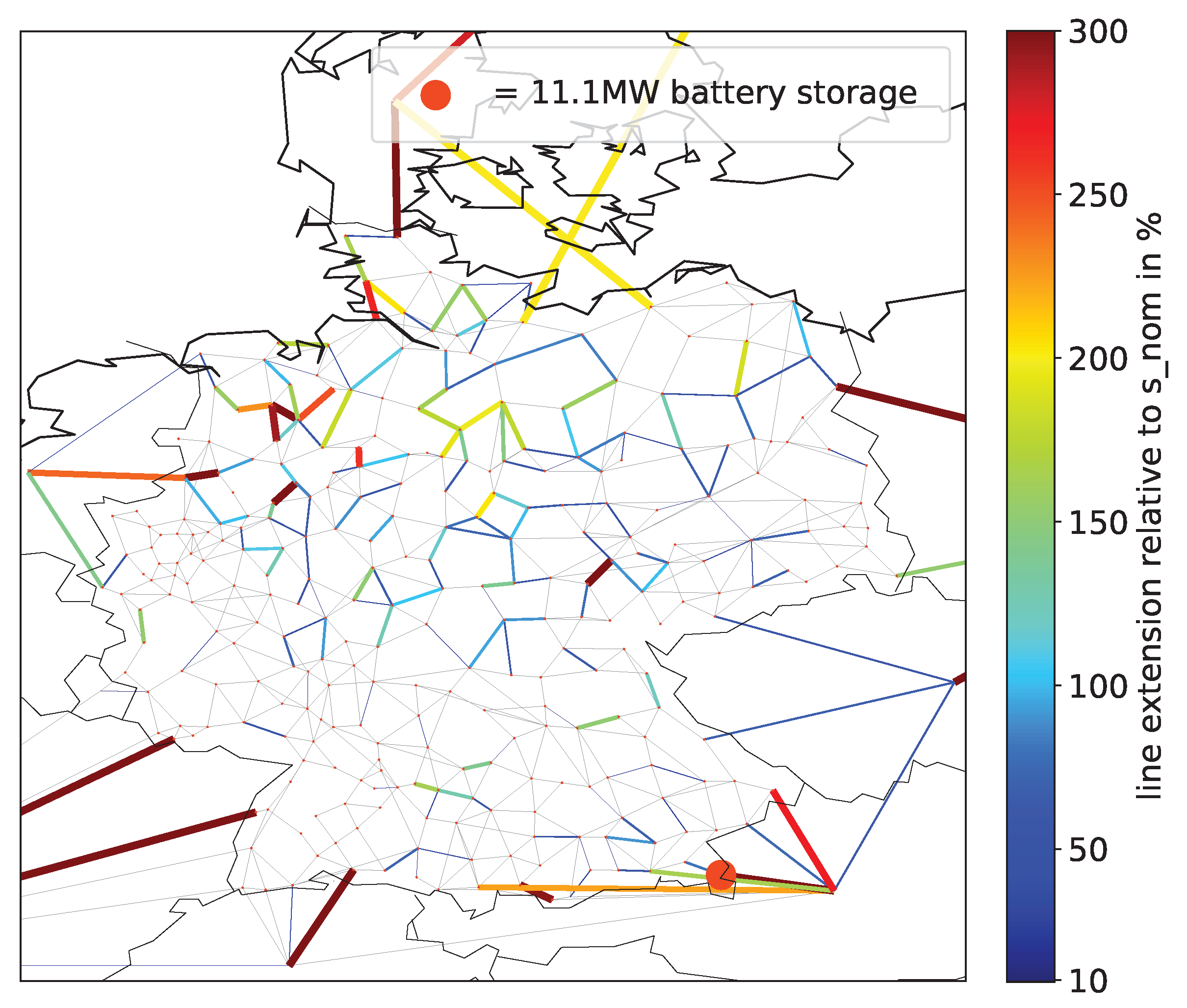
In a mid-term scenario for the year 2035, storage expansion is not an economically feasible option. For a 100% renewable power system in Germany 14 GW storage and 114 GVA grid expansion are co-optimal considering an EHV and HV grid model. Taking into account all voltage levels, total grid expansion investment of 18.6 bn EUR and storage expansion expenses of 11.1 bn EUR are cost-efficient.
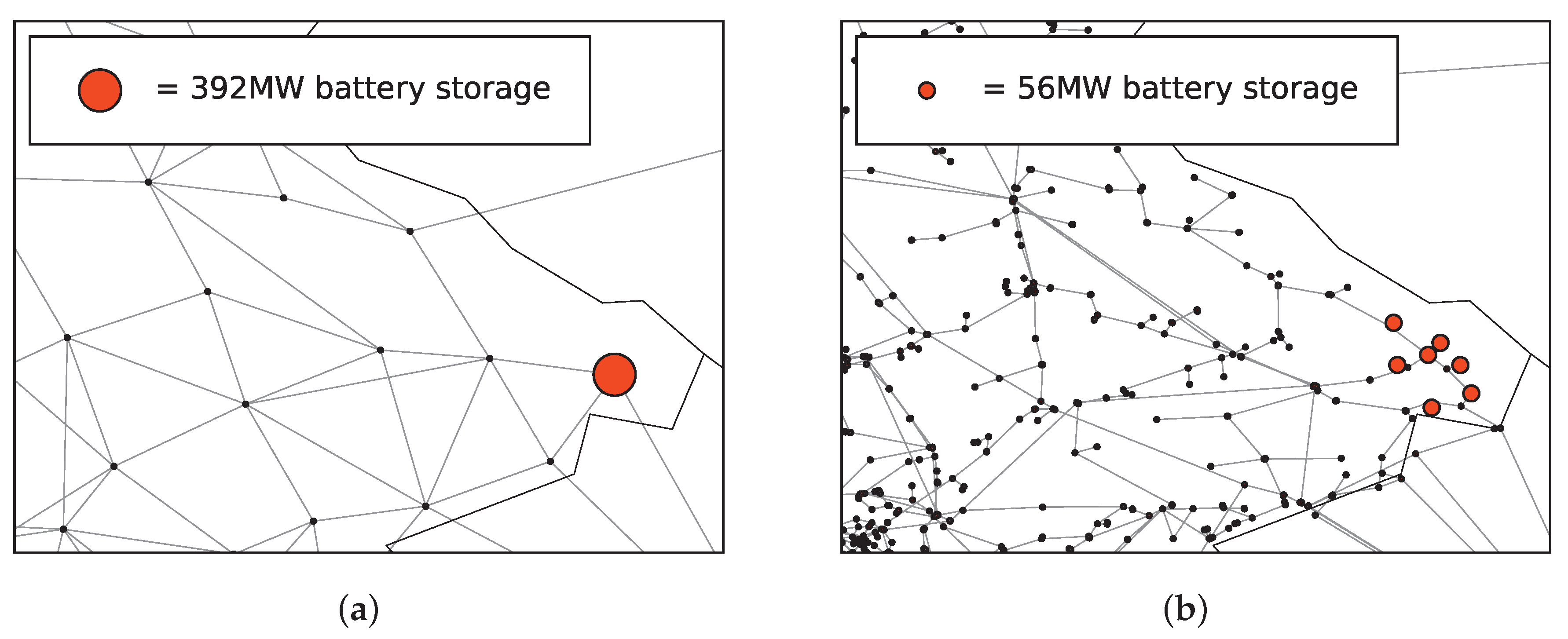
Due to the unidirectional top-down approach the cost-efficient usage of flexibility options i.e., storage expansion and curtailment is limited by the top-level results. Thus, the results for the MV and LV level are twofold. In the eGo 100 scenario the battery storage distribution method leads to a considerably high average reduction of grid expansion costs by 22% concerning the particular MV grids where the decentral battery storage units at the HV/MV connections are also economically feasible for the overall system. Only for 0.9% of all MV grids in Germany this prerequisite was given. Accordingly, the overall investment cost saving was only marginal. In this context, the optimal usage of curtailment did also not reduce the overall MV grid expansion costs significantly although in some grids the cost savings are reaching 30%. Reasons for this effect have been discussed and need to be further analysed.
Comparing the results to grid expansion costs derived by a state of the art worst-case approach, substantial savings depending on the scenario of about 50% were calculated. It can be concluded that the usage of realistic, spatially differentiated time series instead of using general simultaneity factors leads to significant saving potential for distribution grid planning. Nevertheless, this outcome is biased by a linear downscaling of the potential weather-dependent generation time series, minimizing potential and relevant worst cases. As a future research it will be a task to find a more sophisticated correction method which would reflect the weather behavior more accurately. Further research will also be directed toward including the expected electrification of the heat and mobility sectors in the future scenarios that might significantly increase the load in the distribution grids. This could further increase the relevance of an integrated grid planning in order to leverage the flexibility potential these new loads could provide and keep resulting grid expansion needs at a minimum.

Author Contributions

The first idea for the paper developed U.P.M. The further conceptualization was mainly realized by U.P.M. and G.P. The methods and models concerning the EHV and HV level were essentially developed by U.P.M., W.-D.B., J.B. B.S. and G.P. focused on the method and model development for the MV and LV level. M.S. being guided by U.P.M., B.S. and G.P. created the HV-MV interface. The software implementation was similarly distributed. In particular S.G. implemented the disaggregation method being instructed by U.P.M. The original draft was written by all authors except G.P. J.B. and B.S. drafted the state of the art, W.-D.B., U.P.M., M.S., S.G. and B.S. wrote the different parts of the Methods section. Introduction, Results, Discussion, Conclusion and Abstract was written by U.P.M. J.B., B.S. and U.P.M. critically reviewed the paper. Visualization was mainly done by U.P.M. and B.S. The research was coordinated by U.P.M. The funding for the underlying research project was originally acquired by U.P.M. and G.P. (among others).

Funding

This research was conducted as part of the open_eGo project (see also https://openegoproject.wordpress.com/), which was supported by the German Federal Ministry for Economic Affairs and Energy under the funding code: 0325881A-E.

Acknowledgments

The authors thank the many researchers and students who have contributed to the open_eGo project making this research possible. In particular we thank Ilka Cussmann, Clara Büttner, Jonathan Amme, Jochen Bühler, Ludwig Hülk, Martin Glauer and Lukas Wienholt.

Conflicts of Interest

The authors declare no conflict of interest.

References

  1. Bundesministerium für Wirtschaft und Energie. Gesetz für den Ausbau erneuerbarer Energien (Erneuerbare- Energien-Gesetz—EEG 2017); Bundesministerium für Wirtschaft und Energie: Berlin, Germany, 2017. [Google Scholar]
  2. Büchner, J.; Katzfey, J.; Floercken, O.D.; Moser, A.; Schuster, H.; Dierkes, S.; van Leeuwen, T.; Verheggen, L.; Uslar, M.; van Amelsvoort, M. Moderne Verteilernetze für Deutschland (Verteilernetzstudie). 2014. Available online: https://www.bmwi.de/Redaktion/DE/Publikationen/Studien/verteilernetzstudie.pdf?__blob=publicationFile&v=5 (accessed on 30 May 2019).
  3. Agricola, A.C.; Höflich, B.; Richard, P.; Völker, J.; Rehtanz, C.; Greve, M.; Gwisdorf, B.; Kays, J.; Noll, T.; Schwippe, J.; et al. Ausbau- und Innovationsbedarf der Stromverteilnetze in Deutschland bis 2030 (kurz: Dena-Verteilnetzstudie): Endbericht. 2012. Available online: https://shop.dena.de/fileadmin/denashop/media/Downloads_Dateien/esd/9100_dena-Verteilnetzstudie_Abschlussbericht.pdf (accessed on 30 May 2019).
  4. Van Leeuwen, T.; Dierkes, S.; Verheggen, L.; Schuster, H.; Köhne, F.; Moser, A. Ermittlung von Transitflüssen im Hochspannungsnetz durch mehrere Verknüpfungspunkte mit dem Übertragungsnetz. In Proceedings of the 13. Symposium Energieinnovation, Graz, Austria, 12–14 February 2014. [Google Scholar]
  5. Müller, U.P.; Cussmann, I.; Wingenbach, C.; Wendiggensen, J. AC Power Flow Simulations within an Open Data Model of a High Voltage Grid. In Advances and New Trends in Envrionmental Informatics; Wohlgemuth, V., Fuchs-Kittowski, F., Wittmann, J., Eds.; Springer International Publishing Switzerland: Zurich, Switwerland, 2016; pp. 181–191. [Google Scholar]
  6. Müller, U.; Wienholt, L.; Cussmann, I. The role of the high voltage power level in future power systems and their modelling. In Proceedings of the Smart Energy Systems and Technologies Conference, SEST 2018, Sevilla, Spain, 10–12 September 2018. [Google Scholar] [CrossRef]
  7. 50Hertz Transmission GmbH; Amprion GmbH; TenneT TSO GmbH; TransnetBW GmbH (ÜNB). Netzentwicklungsplan Strom 2025, Version 2015—Erster Entwurf der Übertragungsnetzbetreiber. 2015. Available online: https://www.netzentwicklungsplan.de/sites/default/files/paragraphs-files/NEP_2025_1_Entwurf_Teil1_0.pdf (accessed on 30 May 2019).
  8. Bruckner, H.K.T. Flexibility requirements of renewable energy based electricity systems—A review of research results and methodologies. Renew. Sustain. Energy Rev. 2016, 53, 10–22. [Google Scholar] [CrossRef]
  9. Hörsch, J.; Brown, T. The role of spatial scale in joint optimisations of generation and transmission for European highly renewable scenarios. In Proceedings of the 2017 14th International Conference on the European Energy Market (EEM), Dresden, Germany, 6–9 June 2017; pp. 1–7. [Google Scholar] [CrossRef]
  10. Brown, T.; Schlachtberger, D.; Kies, A.; Schramm, S.; Greiner, M. Synergies of sector coupling and transmission reinforcement in a cost-optimised, highly renewable European energy system. Energy 2018, 160, 720–739. [Google Scholar] [CrossRef] [Green Version]
  11. Pfenninger, S.; Hirth, L.; Schlecht, I.; Schmid, E.; Wiese, F.; Brown, T.; Davis, C.; Gidden, M.; Heinrichs, H.; Heuberger, C.; et al. Opening the black box of energy modelling: Strategies and lessons learned. Energy Strategy Rev. 2018, 19, 63–71. [Google Scholar] [CrossRef]
  12. Hilpert, S.; Günther, S.; Kaldemeyer, C.; Krien, U.; Pleßmann, G.; Wiese, F.; Wingenbach, C. Addressing energy system modelling challenges: The contribution of the Open Energy Modelling Framework (oemof). Preprints 2017. [Google Scholar] [CrossRef]
  13. Wiese, F.; Bökenkamp, G.; Wingenbach, C.; Hohmeyer, O. An open source energy system simulation model as an instrument for public participation in the development of strategies for a sustainable future. Wiley Interdiscip. Rev. Energy Environ. 2014, 3, 490–504. [Google Scholar] [CrossRef]
  14. Müller, U.; Wienholt, L.; Kleinhans, D.; Cussmann, I.; Bunke, W.D.; Pleßmann, G.; Wendiggensen, J. The eGo grid model: An open source approach towards a model of German high and extra-high voltage power grids. J. Phys.: Conf. Ser. 2018, 977, 012003. [Google Scholar] [CrossRef]
  15. Wingenbach, M. Integration sozial-ökologischer Faktoren in die Energiesystemmodellierung - am Beispiel von Entwicklungspfaden für den Windenergieausbau in Deutschland. Ph.D. Thesis, Europa-Universität Flensburg, Flensburg, Germany, 2018. Available online: https://www.zhb-flensburg.de/fileadmin/content/spezial-einrichtungen/zhb/dokumente/dissertationen/wingenbach/wingenbach-dissertation.pdf (accessed on 30 May 2019).
  16. 50Hertz Transmission GmbH; Amprion GmbH; TenneT TSO GmbH; TransnetBW GmbH. Netzentwicklungsplan Strom. 2018. Available online: https://www.netzentwicklungsplan.de/de/netzentwicklungsplaene (accessed on 30 May 2019).
  17. Chen, Y.; Glaesemann, K.; Fitzhenry, E. Contingency Analysis Post-Processing With Advanced Computing and Visualization. IFAC-PapersOnLine 2017, 50, 55–60. [Google Scholar] [CrossRef]
  18. Heylen, E.; Ovaere, M.; Proost, S.; Deconinck, G.; Hertem, D.V. A multi-dimensional analysis of reliability criteria: From deterministic N-1 to a probabilistic approach. Electr. Power Syst. Res. 2019, 167, 290–300. [Google Scholar] [CrossRef]
  19. Posser, H.; Bala, A. Praxishandbuch Netzplanung und Netzausbau: Die Infrastrukturplanung der Energiewende in Recht und Praxis; de Gruyter: Berlin, Germany, 2013. [Google Scholar]
  20. Natemeyer, H. Modellierung der Betriebsführung elektrischer Übertragungsnetze für Netzplanungsprozesse; Dissertation in Aachener Beiträge zur Hochspannungstechnik, Band 50; Verlagshaus Mainz GmbH: Aachen, Germany, 2017. [Google Scholar]
  21. Birbalta, S. Application of a Network Reduction Approach on an Energy System Model and the Impact of Different Node Aggregations on the Curtailment of Renewable Energy Generation. Bachelor’s Thesis, Karlsruhe Institute of Technology, Karlsruhe, Germany, 2015. [Google Scholar]
  22. Rüberg, S. Strategische Netzausbauplanung in vermaschten Drehstromnetzen unter besonderer Berücksichtigung der Hochspannungsgleichstromübertragung; Dissertation in Dortmunder Beiträge zu Energiesystemen, Energieeffizienz und Energiewirtschaft, Band 1; Shaker Verlag GmbH: Aachen, Germany, 2017. [Google Scholar]
  23. Eickmann, J.; Priebe, J.; Moser, A. Einfluss des Unit-Commitments im Redispatch. In Proceedings of the EnInnov 2016, 14. Symposium Energieinnovation, Technische Universität Graz, Graz, Austria, 10–12 February 2016. [Google Scholar]
  24. Scheufen, M. Mehrstufige Strukturoptimierung für Höchstspannungsnetze; Dissertation in Aachener Beiträge zur Hochspannungstechnik, Band 44; Verlagshaus Mainz GmbH: Aachen, Germany, 2016. [Google Scholar]
  25. Federal Ministry of Justice and Consumer Protection. Law on Electricity and Gas Supply (Energiewirtschaftsgesetz - EnWG). 2005. Available online: https://www.gesetze-im-internet.de/enwg_2005/BJNR197010005.html (accessed on 30 May 2019).
  26. German Institute for Standardisation (DIN). Voltage Characteristics of Electricity Supplied by Public Distribution Networks, German version EN 50160:2010 + Cor.: 2010; DIN: Berlin, Germany, 2011. [Google Scholar]
  27. Bundesverband der Energie- und Wasserwirtschaft e.V. (BDEW). Technische Richtlinie Erzeugungsanlagen am Mittelspannungsnetz; BDEW: Berlin, Germany, 2008. [Google Scholar]
  28. Verband der Elektrotechnik Elektronik Informationstechnik e. V. (VDE). VDE-Anwendungsregel; VDE-AR-N4105:2011-08; Erzeugungsanlagen am Niederspannungsnetz—Technische Mindestanforderungen für Anschluss und Parallelbetrieb von Erzeugungsanlagen am Niederspannungsnetz; VDE: Frankfurt am Main, Germany, 2011. [Google Scholar]
  29. Association for Electrical, Electronic & Information Technology (VDE). DIN EN 60076-1: Power Transformers—Part 2: Temperature Rise for Liquid-Immersed Transformers; Beuth Verlag: Berlin, Germany, 2011. [Google Scholar]
  30. Association for Electrical, Electronic & Information Technology (VDE). DIN VDE 0276-603: Power Cables—Part 603: Distribution Cables of Rated Voltage 0,6/1 kV; Beuth Verlag: Berlin, Germany, 2011. [Google Scholar]
  31. Rehtanz, C.; Greve, M.; Häger, U.; Hagemann, Z.; Kippelt, S.; Kittl, C.; Kloubert, M.L.; Pohl, O.; Rewald, F.; Wagner, C. Verteilnetzstudie für das Land Baden-Württemberg. 2017. Available online: https://um.baden-wuerttemberg.de/fileadmin/redaktion/m-um/intern/Dateien/Dokumente/5_Energie/Versorgungssicherheit/170413_Verteilnetzstudie_BW.pdf (accessed on 30 May 2019).
  32. Verordnung über die Anreizregulierung der Energieversorgungsnetze (Anreizregulierungsverordnung—ARegV). 2007. Available online: https://www.gesetze-im-internet.de/aregv/BJNR252910007.html (accessed on 30 May 2019).
  33. Harnisch, S.; Steffens, P.; Thies, H.H.; Monscheidt, J.; Münch, L.; Böse, C.; Gemsjäger, B. Planungs und Betriebsgrundsätze für ländliche Verteilungsnetze—Leitfaden zur Ausrichtung der Netze an ihren zukünftigen Anforderungen; Technical Report; Bergische Universität Wuppertal; Siemens AG: Munich, Germany, 2016. [Google Scholar]
  34. Agora Energiewende. Stromverteilnetze für die Energiewende. 2014. Available online: https://www.agora-energiewende.de/fileadmin2/Projekte/2013/Stromverteilnetze-fuer-die-zukunft/Agora_Stromverteilnetze_fuer_die_Energiewende_Stakeholder-Dialog_web.pdf (accessed on 30 May 2019).
  35. Patzak, S. Ermittlung von Planungsrelevanten Netznutzungsfällen für Elektrische Netze. Ph.D. Thesis, RWTH Aachen, Aachen, Germany, 2017. [Google Scholar]
  36. Pilo, F.; Jupe, S.; Silvestro, F.; Bakari, K.; Abbey, C. Planning and Optimization Methods for Active Distribution Systems; Technical Report August; CIGRE: Paris, France, 2014. [Google Scholar]
  37. Rippel, K.M.; Wiede, T.; Meinecke, M.; König, R. Netzentwicklungsplan Strom 2030, Version 2017—Erster Entwurf der Übertragungsnetzbetreiber. 2017. Available online: https://www.netzentwicklungsplan.de/sites/default/files/paragraphs-files/NEP_2030_1_Entwurf_Teil1_0.pdf (accessed on 30 May 2019).
  38. Kays, J. Agent-based Simulation Environment for Improving the Planning of Distribution Grids. Ph.D. Thesis, Technische Universität Dortmund: Sierke Verlag, Göttingen, Germany, 2014. [Google Scholar]
  39. Georgilakis, P.S.; Hatziargyriou, N.D. A review of power distribution planning in the modern power systems era: Models, methods and future research. Electr. Power Syst. Res. 2015, 121, 89–100. [Google Scholar] [CrossRef]
  40. Resch, M.; Bühler, J.; Klausen, M.; Sumper, A. Impact of operation strategies of large scale battery systems on distribution grid planning in Germany. Renew. Sustain. Energy Rev. 2017, 74, 1042–1063. [Google Scholar] [CrossRef] [Green Version]
  41. Hülk, L.; Wienholt, L.; Cußmann, I.; Müller, U.P.; Matke, C.; Koetter, E. Allocation of annual electricity consumption and power generation capacities across multi voltage levels in a high spatial resolution. Int. J. Sustain. Energy Plan. Manag. 2017, 13, 79–92. [Google Scholar] [CrossRef]
  42. Amme, J.; Pleßmann, G.; Bühler, J.; Hülk, L.; Kötter, E.; Schwaegerl, P. The eGo grid model: An open-source and open-data based synthetic medium-voltage grid model for distribution power supply systems. J. Phys.: Conf. Ser. 2018, 977, 012007. [Google Scholar] [CrossRef]
  43. Wienholt, L.; Müller, U.; Bartels, J. Optimal Sizing and Spatial Allocation of Storage Units in a High-Resolution Power System Model. Energies 2018, 11, 3365. [Google Scholar] [CrossRef]
  44. ZNES Flensburg and DLR VE Oldenburg. eTraGo—Optimization of Flexibility Options for Transmission Grids Based on PyPSA. 2018. Available online: https://github.com/openego/eTraGo (accessed on 30 May 2019).
  45. RLI Berlin. eDisGo—Optimization of Flexibility Options and Grid Expansion for Distribution Grids Based on PyPSA. 2018. Available online: https://github.com/openego/eDisGo (accessed on 30 May 2019).
  46. ZNES Flensburg. eGo—A Cross-Grid-Level Electricity Grid and Storage Optimization Tool. Available online: https://doi.org/10.5281/zenodo.2151842 (accessed on 30 May 2019).
  47. OpenStreetMap Contributors. OpenStreetMap. Available online: https://www.openstreetmap.org (accessed on 30 May 2019).
  48. IKS OvGU Mageburg and DLRVE Oldenburg and ZNES Flensburg and RLI Berlin. OpenEnergy-Platform (OEP). 2018. Available online: http://openenergy-platform.org (accessed on 30 May 2019).
  49. Glauer, M.; Günther, S.; Huelk, L.; Bunke, W.D. An Open Database Concept for Open Energy Modelling. In InviroInfo—From Science to Society: The Bridge Provided by Environmental Informatics: Adjunct Proceedings of the 31st Edition of the EnviroInfo; Otjacques, B., Hitzelberger, P., Naumann, S., Wohlgemuth, V.E., Eds.; Shaker Verlag: Aachen, Germany, 2017; p. 149. [Google Scholar]
  50. ZNES Flensburg, RLI Berlin, DLR VE Oldenburg and IKS OvGU Mageburg. Dataprocessing—Open_ego’s (geo)Data Processing, Database Setup, Data Validation, 2018. Available online: https://github.com/openego/data_processing (accessed on 30 May 2019).
  51. Amme, J.; Pleßmann, G. Dingo—Distribution Network Generator, 2018. Available online: https://github.com/openego/ding0 (accessed on 30 May 2019).
  52. Wuppertal Institute and DLR Institute of Networked Energy Systems. osmTGmod. Available online: https://github.com/openego/osmTGmod (accessed on 30 May 2019).
  53. Kerber, G. Aufnahmefähigkeit von Niederspannungsverteilnetzen für die Einspeisung aus Photovoltaikkleinanlagen. Ph.D. Thesis, Technische Universität München: Der Andere Verlag, Tönning, Germany, 2011. [Google Scholar]
  54. Bretschneider, P.; Karstädt, F.; Flemming, S.; Pflugradt, S. Studie zu lokalen Energiespeicherbedarfen: Analyse und Prognose der Technologien und Anwendungsfelder thermischer und elektrischer Energiespeicher auf Nieder und Mittelspannungsebene. 2014. Available online: http://www.thega.de/energiespeicherstudie/ (accessed on 18 April 2019).
  55. Krien, U.; Oemof Developing Group. Feedinlib—Time Series of Pv or Wind Power Plants, 2016. Available online: https://github.com/oemof/feedinlib (accessed on 30 May 2019).
  56. Geyer, B.; Rockel, B. CoastDat-2 COSMO-CLM Atmospheric Reconstruction, 2013. Available online: https://doi.org/10.1594/WDCC/coastDat-2_COSMO-CLM (accessed on 30 May 2019).
  57. Geyer, B. High-resolution atmospheric reconstruction for Europe 1948–2012: coastDat2. Earth Syst. Sci. Data 2014, 6, 147. [Google Scholar] [CrossRef]
  58. Bundesnetzagentur (BNetzA). EEG-Anlagenstammdaten (außer PV-Gebäudeanlagen); Bundesnetzagentur: Bonn, Germany, 2018. [Google Scholar]
  59. Bunke, W.D.; Söthe, M.; Christ, M.; Kaldemeyer, C. (Fl)ensburg (En)ergy (S)cenarios—Open_eGo Scenarios for 2014/2035/2050, 2017. Available online: doi:10.17605/OSF.IO/BPF36 (accessed on 30 May 2019).
  60. e Highway2050. e-HIGHWAY 2050 Modular Development Plan of the Pan-European Transmission System 2050—Database per Country. 2015. Available online: http://www.e-highway2050.eu/fileadmin/documents/Results/e-Highway_database_per_country-08022016.xlsx (accessed on 30 May 2019).
  61. Steffens, P. Innovative Planungsgrundsätze für ländliche Mittelspannungsnetze. Ph.D. Thesis, Bergischen Universität Wuppertal, 2018. Available online: http://elpub.bib.uni-wuppertal.de/servlets/DerivateServlet/Derivate-7535/de1801.pdf (accessed on 30 May 2019).
  62. Heuck, K.; Dettmann, K.D.; Schulz, D. Elektrische Energieversorgung: Erzeugung, Übertragung und Verteilung elektrischer Energie für Studium und Praxis; Springer Fachmedien Wiesbaden: Wiesbaden, Germany, 2013. [Google Scholar] [CrossRef]
  63. FGH. Technischer Bericht 302—Ein Werkzeug zur Optimierung der Störungsbeseitigung für Planung und Betrieb von Mittelspannungsnetzen. 2008. Available online: https://docplayer.org/39734520-Technischer-bericht-302.html (accessed on 30 May 2019).
  64. Pedregosa, F.; Varoquaux, G.; Gramfort, A.; Michel, V.; Thirion, B.; Grisel, O.; Blondel, M.; Prettenhofer, P.; Weiss, R.; Dubourg, V.; et al. Scikit-learn: Machine learning in Python. J. Mach. Learn. Res. 2011, 12, 2825–2830. [Google Scholar]
  65. VanderPlas, J. Python Data Science Handbook: Essential Tools for Working with Data; O’Reilly Media, Inc.: Sebastopol, CA, USA, 2016. [Google Scholar]
  66. Brown, T.; Hörsch, J.; Schlachtberger, D. PyPSA: Python for Power System Analysis. J. Open Res. Softw. 2018, 6, 4. [Google Scholar] [CrossRef]
  67. Erlach, B.; Lunz, B.; Merzkirch, M. Energiespeicher Technologiesteckbrief zur Analyse Flexibilitaetskonzepte für die Stromversorgung 2050. 2015. Available online: https://www.acatech.de/wp-content/uploads/2018/03/ESYS_Technologiesteckbrief_Energiespeicher.pdf (accessed on 30 May 2019).
  68. ACER/CEER. Annual Report on the Results of Monitoring the Internal Electricity Markets in 2015. 2016. Available online: http://www.acer.europa.eu/Official_documents/Acts_of_the_Agency/Publication/ACER%20Market%20Monitoring%20Report%202015%20-%20ELECTRICITY.pdf (accessed on 30 May 2019).
  69. Knorr, K.; Zimmermann, B.; Kirchner, D.; Speckmann, M.; Spieckermann, R.; Widdel, M.; Wunderlich, M.; Mackensen, R.; Rohrig, K.; Steinke, F.; et al. Kombikraftwerk 2—Abschlussbericht. 2014. Available online: http://www.kombikraftwerk.de/fileadmin/Kombikraftwerk_2/Abschlussbericht/Abschlussbericht_Kombikraftwerk2_aug14.pdf (accessed on 30 May 2019).
  70. Rendel, T. Erweiterung und Plausibilisierung eines Modells für die integrierte Simulation des europäischen Verbundnetzes und Strommarktes. Ph.D. Thesis, Gottfried Wilhelm Leibniz Universität Hannover, Hannover, Germany, 2015. [Google Scholar]
  71. Han, J.; Kamber, M.; Tung, A.K. Spatial Clustering Methods in Data Mining. 2001. Available online: https://www.comp.nus.edu.sg/~atung/publication/gkdbk01.pdf (accessed on 30 May 2019).
  72. Linsenmeier, M. Estimating costs of extending electricity distribution networks in Germany. Master’s Thesis, Humboldt-Universität zu Berlin, 2017. Available online: https://reiner-lemoine-institut.de/wp-content/publications/Abschlussarbeiten/2018_10_MA_Linsenmeier.pdf (accessed on 30 May 2019).
  73. Tonkoski, R.; Lopes, L.A.C.; El-Fouly, T.H.M. Coordinated active power curtailment of grid connected PV inverters for overvoltage. IEEE Trans. Sustain. Energy 2011, 2, 139–147. [Google Scholar] [CrossRef]
  74. Agricola, A.C.; Seidl, H.; Mischinger, S.; Rehtanz, P.C.; Greve, M.; Häger, U.; Hilbrich, D.; Kippelt, S.; Kubis, A.; Liebenau, V.; et al. Dena—Studie Systemdienstleistungen 2030. Sicherheit und Zuverlässigkeit einer Stromversorgung mit hohem Anteil erneuerbarer Energien: Endbericht. 2014. Available online: https://www.dena.de/fileadmin/dena/Dokumente/Pdf/9094_dena-Studie_Systemdienstleistungen_2030.pdf (accessed on 30 May 2019).
  75. Cebulla, F. Langfristiger Speicher-und Flexibilitätsbedarf in Europa; EUM Fachtagung; German Aerospace Center: Cologne, Germany, 2016. [Google Scholar]
  76. Droste-Franke, B. Future Storage and Balancing Demand—Ranges, Significance and Potential Improvements of Estimations. In Proceedings of the 8th IRES Conference, Berlin, Germany, 18–20 November 2013. [Google Scholar]
  77. Cebulla, F. Stromspeicherbedarf in europäischen Langfristszenarien- Eine Analyse des Einflusses unterschiedlicher energiewirtschaftlicher Rahmenbedingungen. In 11. VDI-Fachtagung Optimierung in der Energiewirtschaft; VDI-Berichte: Karlsruhe, Germany, 2015; Volume 2266, pp. 3–14. [Google Scholar]
  78. Braun, M.; Krybus, I.; Becker, H.; Bolgaryn, R.; Dasenbrock, J.; Gauglitz, P.; Horst, D.; Pape, C.; Scheidler, A.; Ulffers, J. Verteilnetzstudie Hessen 2024–2034: Studie im Auftrag des Hessischen Ministeriums für Wirtschaft, Energie, Verkehr und Landesentwicklung. 2018. Available online: https://www.house-of-energy.org/mm/2018_Verteilnetzstudie_Hessen_2024_bis_2034.pdf (accessed on 30 May 2019).
  79. Bundesministerium für Wirtschaft und Energie BMWi. Gesamtausgabe der Energiedaten—Datensammlung des BMWi (Sheet 20); Bundesministerium für Wirtschaft und Energie BMWi: Berlin, Germany, 2017. [Google Scholar]
  80. Schlemminger, M. Modellierung von Redispatch-Maßnahmen im deutschen Hoch- und Höchstspannungsnetz. Master’s Thesis, Europa-Universität Flensburg, Flensburg, Germany, 2018. [Google Scholar]
  81. Park, H.S.; Jun, C.H. A simple and fast algorithm for K-medoids clustering. Expert Syst. Appl. 2009, 36, 3336–3341. [Google Scholar] [CrossRef]
  82. Biener, W.; Senkpiel, C.; Shammugam, S.; Garcia Rosas, K.R.; Linke, M.; Eibl, O. Impact of grid reduction on modelling accuracy of line usage rates. J. Phys.: Conf. Ser. 2018, 977, 012001. [Google Scholar] [CrossRef]
  83. Hörsch, J.; Ronellenfitsch, H.; Witthaut, D.; Brown, T. Linear optimal power flow using cycle flows. Electr. Power Syst. Res. 2018, 158, 126–135. [Google Scholar] [CrossRef] [Green Version]
  84. Schlachtberger, D.; Brown, T.; Schramm, S.; Greiner, M. The benefits of cooperation in a highly renewable European electricity network. Energy 2017, 134, 469–481. [Google Scholar] [CrossRef] [Green Version]
  85. Milano, F. Power System Modelling and Scripting; Springer Science & Business Media: New York, NY, USA, 2010. [Google Scholar]
  86. Müller, U.P.; Schachler, B.; Bunke, W.D.; Bartels, J.; Glauer, M.; Büttner, C.; Günther, S.; Kötter, E.; Cußmann, I.; Hülk, L.; et al. Netzebenenübergreifendes Planungsinstrument—zur Bestimmung des optimalen Netz- und Speicherausbaus in Deutschland—integriert in einer OpenEnergyPlatform. 2019. Available online: https://www.uni-flensburg.de/fileadmin/content/abteilungen/industrial/dokumente/downloads/veroeffentlichungen/forschungsergebnisse/20190426endbericht-openego-fkz0325881-final.pdf (accessed on 30 May 2019).
Figure 1. Installed generation capacities for Germany (GER) and the entire model region (total) per scenario and technology/fuel [59].
Energies 12 02091 g001
Figure 2. The Status Quo grid topology model for the EHV and HV level (a). In (b) one of the 3376 underlying MV grid topologies and its connection to the HV level is displayed. Its location corresponds to the zoom box in (a). The connected generation (except for MV generators in (b)) and demand as well as transformers are not displayed for better visualization. A visualized bus which seems to connect two voltage levels is actually modelled as two buses connected by a transformer (see also [14]).
Energies 12 02091 g002
Figure 3. Exemplary visualization of the E–M algorithm for k-means clustering [65]. During the E-Step, all data points are assigned to the nearest (initially randomly set) cluster center. Afterwards each cluster center is reset to the centroid of its current cluster. These steps are repeated until convergence.
Energies 12 02091 g003
Figure 4. Exemplary allocation of battery storage expansion before (a) and after (b) disaggregation. In (a) the EHV and HV grid is reduced to 300 buses. In (b) the original complete complexity is displayed. For better visualization it was zoomed in to a subregion of southern Bavaria next to the border to the Czech Republic and Austria. The basic grid topology is visualized by grey lines and black buses.
Energies 12 02091 g004
Figure 5. Relative deviation of grid expansion costs of different k cluster approximations compared to the calculation of all MV grids using the simple worst-case method.
Energies 12 02091 g005
Figure 6. MV grid clusters with 600 representative MV grids (black-rimmed) and their weighting for the eGo 100 scenario. The MV grid districts are displayed without any grid topology.
Energies 12 02091 g006
Figure 7. Grid expansion measures to solve overloading and voltage issues in MV and LV grids based on [31].
Energies 12 02091 g007
Figure 8. Linear relation between relative curtailment and bus voltage used to allocate curtailment requirements.
Energies 12 02091 g008
Figure 9. Illustration of the approach of finding the storage size that minimizes the maximum load in a feeder.
Energies 12 02091 g009
Figure 10. Allocation of grid and storage expansion in the EHV and HV level for the scenario NEP 2035. s_nom refers to the original nominal thermal limit capacity of each line. A net 300% extension is synonymous with a new optimized capacity of four times the original capacity.
Energies 12 02091 g010
Figure 11. Allocation of grid and storage expansion in the EHV and HV level for the scenario eGo 100. s_nom refers to the original nominal thermal limit capacity of each line. A net extension of 300% is synonymous with a new optimized capacity of four times the original capacity.
Energies 12 02091 g011
Figure 12. Allocation of grid and storage expansion for a representative MV grid for the scenario eGo 100. Orange colored nodes represent battery storage units. Color of other nodes and lines represents expansion costs of stations and lines.
Energies 12 02091 g012
Table 1. Grid and storage expansion parameters for the scenarios NEP 2035 and eGo 100 1 based on [67] (storage units), [3] (HV grid) and [7] (EHV grid).
ComponentOvernight CostsUnit EUR/
Overhead Line, 380 kV85MVA*km
Overhead Line, 220 kV290MVA*km
Overhead Line, 110 kV230MVA*km
EHV DC-Link (underground)375MVA*km
DC-Converter200,000MVA
Transformer, 380–220 kV14,166MVA
Transformer, 380–110 kV17,333MVA
Transformer, 220–110 kV7,500MVA
Battery storage, P-E ratio: 1/6918,500/678,000 1 MW
Hydrogen storage, P-E ratio: 1/168890,600/650,600 1 MW
Table 2. Standard equipment for grid expansion in MV and LV grids [3]. a costs include earthwork costs in area with population density of ≤500 people/km 2 . b costs include earthwork costs in area with population density of >500 people/km 2 .
EquipmentOvernight Investment Costs in kEURUnit
MV cable, NA2XS2Y 3 × 1 × 185 RM/2520/80 a /140 b km
LV cable, NAYY 4 × 1 × 1509/60 a /100 b km
HV/MV Transformer, 40 MVA1000-
MV/LV Transformer, 630 kVA10-
Table 3. Allowed equipment load factors used to identify thermal overloading [31].
EquipmentLoad Factor in HLFLoad Factor in RPF
MV cable50%100%
LV cable100%100%
HV/MV Transformer50%100%
MV/LV Transformer100%100%
Table 4. Allowed voltage deviations used to identify voltage issues [31].
Voltage LevelVoltage Deviation in HLFVoltage Deviation in RPF
MV1.5%5.0%
MV/LV2.0%1.5%
LV6.5%3.5%
Table 5. Used Simultaneity factors of loads and generators in MV and LV grids for calculation of worst-case grid expansion costs based on [3].
Design CaseLoadGeneration
HLF100%0%
RPF15% (MV)/10% (LV)85% (Solar)/100% (Other)
Table 6. Comparison of grid expansion costs per scenario in the MV and LV level based on a calculation of 600 cluster grids. The costs of the transformation levels HV-MV and MV-LV are included in the MV and LV level.
ScenarioGrid Investment bn EUR per Voltage LevelComparison to Flex in %
MVLV
NEP 2035Flex8.171.69-
Reference8.171.70+0
Worst-Case-60012.62.60+54
Worst-Case-359112.52.40+51
eGo 100Flex10.22.39-
Reference10.32.42+0
Worst-Case-60015.33.76+51
Worst-Case-359115.23.62+49
Table 7. Overview of overnight investment costs for grid and storage expansion for each scenario and grid level.The MV+LV results refer to the Flex approach. Transformer costs are included in each aggregated grid level - HV/MV transformer are assigned to the MV+LV level.
ScenarioGrid LevelGrid Investment bn EURStorage Investment bn EUR
BatteryHydrogen
NationalCross-BorderAbroadNationalAbroadNationalAbroad
NEP 2035EHV+HV3.11.52.70.013000
MV+LV9.9------
eGo 100EHV+HV4.11.72.82.009.12.2
MV+LV12.6--0.014---

