Simulation-Based Comparison Between the Thermal Behavior of Coaxial and Double U-Tube Borehole Heat Exchangers

Abstract

In this study, the thermal behavior of the coaxial and double U borehole heat exchangers was investigated using numerical simulations in both the long- and short-term. As a reference for borehole heat exchanger specifications, the existing coaxial and double U probes of a geothermal heat pump installed within the Horizon 2020 research project named “Cheap GSHPs” were considered. Nine years of simulations revealed that when borehole heat exchangers are subjected to a balanced thermal load, and intermittent operating modes of the ground source heat pump system are set, the coaxial pipes’ configuration provides better thermal performance due to the higher thermal capacitance of the heat-carrier fluid and the lower borehole thermal resistance. The analysis was conducted considering two different types of ground with different thermal conductivity values. As result, the more conductive ground type highlights the higher yield of the coaxial probe.

1. Introduction

Technological innovations in the field of ground heat exchangers (GHEs) sizing and design can help improve their thermal performance and, consequently, to reduce the length necessary to satisfy building energy needs. This reduction decreases the installation costs, which are particularly high for vertical systems. Several works have recently been conducted on coaxial GHEs, which consist of an inner central pipe and an annular channel in direct contact with the surrounding ground. In the past, this coaxial geometry was studied by Oliver and Braud [1], who derived a closed form analytical solution under steady state operation considering an isothermal ground surface one meter away from the axis of the borehole heat exchanger. Field tests were performed on a 47.7 m vertical tube-in-tube by Mei and Fischer [2], who used the data collected to validate a mathematical model, and the computer model was then used to study the effects of variations in heat-exchanger length, diameter, and flow rate on the heat-exchanger performance. Other field tests on several closed and open annular coaxial GHEs with and without external pipes were described [3]. In particular, small-size coaxial heat exchangers (SCGHEs) with an external stainless steel tube, directly driven into the soil (no borehole is made to install them) up to a depth of about 20 m, were analyzed through finite-element numerical simulations performed using the software package COMSOL Multiphysics (COMSOL AB, Stockholm, Sweden) to evaluate the effects of thermal short-circuiting on the performance of SCGHEs and to determine the changes in the performance of a SCGHE if the flow direction is reversed [4].

The thermal performance of two pipe-in-pipe borehole heat exchangers (BHEs), with one having a partly insulated central pipe, was studied by Acuna and Palm [5] with regard to global and local borehole thermal resistances during several distributed thermal response tests. Both BHEs operated with similar efficiency. Global (effective) borehole resistance was about 0.03 K∙m/W, whereas local resistance was about 0.01 K∙m/W.

Most of the above mentioned research underlined the potential for efficiency improvements brought about by coaxial BHEs, so other authors comparatively analyzed the pipe-in-pipe GHE and the more conventional double U and single U-tube. Hydraulic performance tests performed by Wood et al. [6] showed that the U-tube achieved transitional-turbulent flow at a glycol flow rate of approximately 0.14 L/s, whereas the flow in the coaxial remained laminar across the glycol flow rate range of 0.05 to 0.25 L/s. Heat pump performance tests demonstrated that the U-tube achieved a COP of at least 0.08 greater than the coaxial loop across the range of glycol flow rates investigated, whereas the heat output was at least 12% greater when using the U-tube. Therefore, they concluded that the coaxial loop in its current form was not seen to provide any performance benefit compared to the U-tube.

Zarrella et al. [7] analyzed enhanced (steel pipes) coaxial heat exchangers in comparison with the common double U-tube using thermal response test measurements under the same conditions. The thermal performance of the enhanced coaxial heat exchanger was better than that of the double U-tube, due especially to a lower (about 83%) borehole thermal resistance. In the short-term, the simulations, performed with the numerical capacity resistance model (CaRM), showed the better thermal behavior of the coaxial heat exchanger due to the thermal capacitance of the heat-carrier fluid, which was six times greater than in the double U-tube.

Design calculations analytically performed by Raymond et al. [8] suggested that at a high flow rate, the borehole thermal resistance of the proposed coaxial GHEs can be below 0.05 K∙m/W, which is significantly below single U-pipe GHEs, but above double U-pipe GHEs. However, the large coaxial GHEs with a high heat storage capacity enabled greater bore length reduction than the double U-pipe GHEs.

Several analytical and numerical models have been developed that can be categorized with regard to the type of the source heat (infinite or finite, linear or not) [9]. Conti [10] conducted analyses to develop plain and convenient expressions to decide the most suitable analytical model for the thermal analysis of the ground in vertical ground-coupled heat pump applications, concluding that the finite line source model [11] can be used for a wide range of space and time scales.

The cylindrical heat source method is another analytical approach [12] that can be used to consider the finite diameter of the BHE. It provides an exact solution of a cylindrical heat source placed in an infinite homogeneous medium, i.e., the ground. In this case as well, the properties of the ground are assumed constant, the axial heat transfer is neglected, and a perfect contact between the cylinder wall and the ground is assumed.

Zanchini et al. [13] focused on improving the thermal performance of long coaxial borehole heat exchangers (CBHEs) by investigating the effects of thermal short-circuiting and flow rate, as well as the constituent materials and the geometrical configuration of the CBHE cross-section. The analysis was performed using finite element simulations, implemented through the software package COMSOL Multiphysics (COMSOL AB, Stockholm, Sweden).

Other numerical models were applied in the evaluation of Thermal Response Tests (TRTs) and in the design of BHEs, where the mean temperature of the fluid is usually approximated by the arithmetic average (T_m) of THE inlet and outlet temperatures. Marcotte and Pasquier [14] proved that considering T_m the borehole thermal resistance is overestimated. The resistance overestimation has a noticeable economic impact. Therefore, they demonstrated with a full three-dimensional (3D) numerical model [15] that a new estimator p-linear average (with parameter p → –1) closely fits the average fluid temperature computed with the model. Accurate 3D simulations of a typical double U-tube BHE working with a constant inlet fluid temperature have been completed by Zanchini et al. [16] through a finite element model implemented in COMSOL Multiphysics (COMSOL AB, Stockholm, Sweden). The results were qualitatively validated by applying the analytical method developed by Zeng et al. [17], and provided new relations that could be used to evaluate T_m.

However, all these analytical and numerical models do not consider the effect of the thermal capacitance of the heat-carrier fluid inside the pipes of the BHE and the variation in the weather conditions at the ground surface, which can significantly affect the thermal behavior, especially that of shallow BHEs. The current study set out to compare the long- and short-term performance of double U-tube and coaxial pipes subjected to a balanced annual thermal load profile over nine years and considering the intermittent operating of the heat pump. This analysis was conducted through simulations performed with a detailed calculation tool, CaRM [18], which considers the climatic conditions at the ground surface, axial heat transfer into both the grouting material and ground, the fluctuations in the heat load, and thus the dynamic thermal behavior of the BHE. This is possible because the model considers the thermal capacitance of both the grouting material and the heat-carrier fluid inside the pipes of the BHE.

2. Method

2.1. Case Study

As a case study, two existing borehole heat exchangers (an enhanced stainless steel 76.60-mm coaxial and a 32-mm double-U), 78 m deep each (L_bore), of a ground source heat pump located in a residential dwelling in Putte (North Belgium) were considered. This is where a real case study of the Cheap GSHPs project [19] is underway. The demonstration system includes four other BHEs (two stainless steel 48.30-mm coaxial, one 32-mm double-U and one stainless steel 76.60-mm coaxial). The layout of the GHEs is shown in Figure 1, in which the two analysed BHEs are represented by red dots.

These BHEs and solar collectors supply a water source heat pump with a nominal thermal capacity of 12 kW in heating mode, which provides the building heating, cooling, and domestic hot water production. The system is equipped with measuring and data logging equipment for online real time monitoring of the entire system. The local geology is presented in Figure 2a. The engineering layout of the system is shown in Figure 2b.

The enhanced coaxial probe consists of a concentric shape composed of two tubes: the inner one composed of polyethylene for the supply and the external one composed of stainless steel for the return. The characteristics of this BHE are reported in

Table 1. Characteristics of the coaxial borehole heat exchanger.

Description	Value
Inner pipe (1)
Inside diameter of pipe (mm)	26.8
Outside diameter of pipe (mm)	40
Thermal conductivity of pipe (W/(m∙K))	0.14
Outer pipe (2)
Inside diameter of pipe (mm)	68.9
Outside diameter of pipe (mm)	76.1
Thermal conductivity of pipe (W/(m∙K))	15.0
Borehole diameter (m)	0.101
Inlet pipe	inner pipe
Grouting material
Thermal conductivity (W/(m∙K))	1.5
Specific heat (J/(kg K))	2500.0
Density (kg/m3)	1400.0

.

The inner tube of this probe does not have the same characteristics of the traditional ones, as it features an insulating foam on the outer part of the inner tube. This foam allows better thermal insulation and consequently reduces the thermal short-circuit between the delivery section and the return annular section. The schematization of the cross-section of the coaxial pipe is shown in Figure 3.

The specifications of the double U-tube BHE, composed of PE-Xa pipes, are reported in

Table 2. Specifications of the double U heat exchanger.

Description	Value
Inside diameter of pipe (mm)	26.2
Outside diameter of pipe (mm)	32.0
Spacing between the pipes (mm)	82.6
Borehole diameter (m)	0.125
Thermal resistance between adjacent pipes (m∙K/W)	0.59
Thermal resistance between opposite pipes (m∙K/W)	0.8
Thermal resistance between the pipe and the bore wall (m∙K/W)	0.25
Grouting material
Thermal conductivity (W/(m∙K))	1.5
Specific heat (J/(kg∙K))	2500.0
Density (kg/m3)	1400.0
Connection 2 U	Parallel

.

2.2. Test Measurements

2.2.1. Thermal Response Test (TRT)

During the first testing phase, a TRT was performed in order to determine the equivalent thermal conductivity of the ground and the borehole thermal resistance (R_b). The test was conducted on both the double U-tube and coaxial pipes using the same boundary conditions in terms of heat injection rate, time duration, and total mass flow rate.

The TRT procedure is based on the infinite line source method to evaluate the equivalent thermal conductivity of the ground. For this, a constant heat injection/extraction rate into the borehole with known depth and radius is set. This heat rate is imposed by a circulating carrier fluid in the BHE, with a certain mass flow rate, so it is possible to determine the fluid temperature development over time at the inlet and outlet at the probe.

In

Table 3. Thermal Response Test (TRT) results.

BHE	Borehole Thermal Resistance, Rb ((m∙K)/W)	Ground Thermal Conductivity, λ (W/(m∙K))
Double U-tube	0.076	2.16
Coaxial pipes	0.036	2.06

, the calculated borehole thermal resistance indicates the improved energy performance of the coaxial BHE compared to the double-U BHE. The equivalent ground thermal conductivity values obtained from the analysis of this test, conducted over 5 days, are also presented.

2.2.2. Weekly Test

Then, a weekly test was performed to monitor the functioning of the two BHEs with the average flow rates and the associated values of Reynolds number (Re) presented in

Table 4. Average flow rates used to perform the tests and the resulting Reynolds number (Re) for the double U-tube and the coaxial pipes.

BHE	Average Flow Rate (L/min)	Re	Re in	Re out
Double U-tube	8.68	2603	-	-
Coaxial pipes	4.79	-	2832	688

.

The heat-carrier fluid (pure water) was moved by the circulator, while the inlet and outlet fluid temperatures at the top of the boreholes and the volumetric fluid flow rate were measured and recorded at 120 s time intervals. The temperatures were monitored with Pt 1000 Class A resistance thermometers (Ifm Electronic, Essen, Germany) (accuracy of ± (0.3 + 0.1% MS) in K), and the volumetric flow rate was measured using an electromagnetic flow meter (accuracy of ± (0.8% MW + 0.5% MEW) in L/min).

In this case study, the objective was to check if the results obtained via the numerical tool CaRM match the measured temperature values. To this purpose, the measured inlet fluid temperature profiles (Figure 4) of the coaxial pipes and the double U-tube were considered as input for CaRM calculation tool to simulate the thermal behavior of the BHEs. The inlet fluid temperature was measured for the real operating conditions of the heat pump; consequently, the heat pump was switched off for some time steps (about 22% of the time) and then started again.

The simulations were performed for a week in 120-s time-steps using at the ground level air temperature and solar radiation measured at the site. The mass flow rates of the heat-carrier fluid were set equal to the average values used for the weekly test (4.79 L/min for the coaxial pipes, 8.68 L/min for the double U-tube). Regarding the ground characteristics: thermal conductivity (λ) was assumed to be 2.11 W/(m∙K), which is the average value between the thermal conductivities obtained via TRT on coaxial pipes and double U- tube; and the volumetric heat capacity (C) was 2.42 MJ/(m³∙K). At the ground level, the following values were applied and assumed to be constant for the entire simulation time: absorptance (a): 0.7, emittance (ε): 0.9, and convection thermal resistance per unit area (R_ext): 0.04 (m²∙K)/W.

As result, the calculated and the experimental outlet fluid temperatures were compared for the coaxial (Figure 5) and the double U (Figure 6) probes. The fluctuations in the simulated outlet fluid temperature in the coaxial probe were greater than in double U-tube, which could be due to the different volumes of the grouting material. The heat transfer rate was plotted in both the figures to better determine the model’s accuracy; the average values of the heat transfer rate per unit borehole length are about 8 and 15 W/m for the coaxial and double U-tube probe, respectively.

It is important to remember that in the time steps, when the heat pump is switched off, the model still calculates the fluid temperatures according to the heat balance of the thermal nodes, and when it starts again, the CaRM tool is able to consider the influences on the ground throughout the previous time steps and the fluctuations of the heat load. The results obtained via CaRM replicate the fluctuations in the measured outlet fluid temperatures. The root mean square error (RMSE) in Equation (1) between the experimental outlet fluid temperature ($T_{out,exp}$) and the corresponding value calculated ($T_{out,sim}$) using CaRM was considered to evaluate the deviation.

$$\mathrm{RMSE}=\sqrt{\frac{{\sum }_{i=1}^{n_{step}}{(T_{out,exp,i}-T_{out,sim,i})}^2}{n_{step}}}$$

(1)

Regarding the 168 hours of simulations, the RMSE values calculated with Equation (1) are 0.37 and 0.23 for the coaxial pipes and double U-tube, respectively. If the first 72 h, characterized by high fluctuations in the experimental outlet fluid temperature, are not considered, the resulting RMSE values decrease to 0.16 and 0.13 for the coaxial pipes and double U-tube, respectively.

2.3. Computer Simulations

2.3.1. Long-Term Analysis

The yield differences between the ground heat exchangers were also determined under variable load conditions with computer simulations. We considered the annual ground load profile shown in Figure 7, representing the hourly heat load extracted or injected by the borehole heat exchanger. This profile is representative of a residential building located in Venice (Italy), with a floor area of around 150 m². The U values of the external walls and the roof were 0.3 W/(m²∙K) and 0.24 W/(m²∙K) respectively, and the glazed surfaces had a thermal transmittance of 1.5 W/(m²∙K). The entire glazed surface was around one-sixth of the floor area and its solar factor (ratio of the total solar energy flux entering through the glass to the incident solar energy flux) was 0.35 and was assumed to be constant during the entire simulation time. The data and shape of the building load profile denote an almost balanced profile.

The amounts of energy exchanged with the ground are similar in absolute value between summer (2200 kWh) and winter (2677 kWh), as shown in Figure 8, and the heating-cooling energy ratio is 1.22.

According to the Köppen-Geiger climate classification, Venice belongs to the group Cfa, so it is characterized by a humid, subtropical climate, with hot and muggy summers and moderately cold winters. The average temperature ranges from 3.5 °C in January to 23 °C in July.

The thermal load profile was considered as the input for CaRM to simulate the thermal behavior of the double U-tube. The simulation was performed for nine years, with a 5-minute calculation time-step.

This simulation was conducted using the following other inputs:

(1)

The mass flow rate of the heat-carrier fluid (pure water) was 0.23 kg/s. This flow develops a transient flow regime for both the double U-tube (since the Reynolds number is 5602) and the coaxial pipes (Re = 2696 in the annulus).

(2)

As main ground characteristics: the ground thermal conductivity (λ) was assumed to be 2.1 W/(m∙K) and the volumetric heat capacity (C) was 2.42 MJ/(m³∙K).

(3)

With regards to the mesh parameters, to model the borehole heat exchangers: (1) in the surface zone and the deep zone, the ground was split into vertical sub-regions with a thickness of 0.25 m each, whereas in the ground surrounding the borehole, the sub-regions were 1 m thick. (2) Each vertical sub-region of the borehole zone was divided into 20 annular regions from the borehole axis to the maximum radius (r_max) of 10 m.

(4)

At the ground level, the following values were applied and assumed to be constant for the entire simulation time: absorptance (a) was 0.7, emittance (ε) was 0.9, and specific surface convective thermal resistance (R_ext) was 0.04 (m²∙K)/W.

Among the results output from the CaRM tool, the temperatures of the heat-carrier fluid at the inlet of the probe were used, step by step, to obtain a profile of inlet temperature for nine years. This last profile (Figure 9) was considered as the input for both the CaRM simulations of coaxial and double U-tube ground heat exchangers, aimed at determining the thermal performance of these probes. As such, the same inlet temperature was assumed at the head of the probes in each time-step, starting with the thermal load profile reported in Figure 7. These simulations were performed with the same inputs as the previous one, but in addition to the 2.1 W/(m∙K), another value of the ground thermal conductivity, 1.1 W/(m∙K), was considered to analyze the thermal performance in two different types of ground.

2.3.2. Short-Term Analysis

A further simulation was performed for each borehole heat exchanger to investigate the thermal behaviors in short-term. In this case, the input signal alternates a one-month heat pump stop period with one operating month in which the fluid inlet temperature is constant at 3 °C (Figure 10). The one-month period “off” is necessary to ensure that the simulated temperature of the surrounding ground can conform to the considered climatic conditions and that the temperature of the transfer fluid inside the borehole heat exchangers can match that of the surrounding ground before starting the heat pump. The other inputs were the same as the simulations performed in the long-term analysis.

3. Results and Discussion

3.1. Long-Term Analysis

The distinct geometries of the two borehole heat exchangers lead to a different thermal behavior, and thereby to an unequal exchange of energy both in heating and cooling mode.

Table 5. Energy exchanged with the ground by the two BHEs during heating and cooling mode in the first, third, and ninth years, assuming λ = 1.1 $\mathrm{W}/\left(\mathrm{m}·\mathrm{K}\right).$

Simulation Year	Energy Exchanged with the Ground (kWh)
	Heating		Cooling
	Coaxial	Double U	Coaxial	Double U
1st	–2222	–2159	1742	1715
3rd	–2173	–2099	1768	1751
9th	–2139	–2027	1794	1808

and

Table 6. Energy exchanged with the ground by the two BHEs during heating and cooling mode of the first, third, and ninth years, assuming λ = 2.1 $\mathrm{W}/\left(\mathrm{m}·\mathrm{K}\right)$.

Simulation Year	Energy Exchanged with the Ground (kWh)
	Heating		Cooling
	Coaxial	Double U	Coaxial	Double U
1st	–3043	-–2863	2432	2307
3rd	–3036	–2876	2443	2304
9th	–3009	–2884	2465	2297

summarize the exchanged energy rates, determined by the simulations, considering the ground thermal conductivity of 1.1 and 2.1 W/(m∙K), respectively.

As a result, assuming λ = 1.1 W/(m∙K), throughout the first year, the energy exchanged with the ground by the coaxial probe was around 2.9% higher than that of the double U-tube considering the entire heating period. During the cooling season, this value was 1.6%. Over the course of the third year, the percentages were 3.5% in heating mode and 0.1% in cooling mode. During the ninth year, the values were 5.5% in heating mode and –0.01% in cooling mode (the energy rate exchanged by the coaxial probe was a little lower than that of the double U-tube).

Considering the ground thermal conductivity of 2.1 W/(m∙K), during the first year, the energy rate exchanged by the coaxial probe was 6.3% higher than the double U during the heating period; 5.4% higher in the cooling season. Over the course of the third year, the percentages were 5.5% in the heating period and 6% in the cooling period. During the ninth year, these values were 4.3% in heating mode; 7.3% in cooling mode.

To analyze in detail the performance of the borehole heat exchangers, the outlet temperature of the heat-carrier fluid at the head of the probes was considered as a relevant output of the CaRM. This was possible because, as mentioned, the mass flow rate, the specific heat, and the inlet fluid temperatures were the same, indicating which of the two probes exchanges more heat with the ground.

In Figure 11, the outlet temperatures of the heat-carrier fluid of the two probes are represented during the third simulated year with a value of ground thermal conductivity of 1.1 (Figure 11a) and 2.1 W/(m∙K) (Figure 11b).

To better understand the difference between the outlet fluid temperatures of the two probes, three reference periods of three hours were considered:

(1)

Period A: During the heating mode when the inlet fluid temperature at the head of the probe is equal to the minimum value (a critical condition because the absorption of energy has minimized the ground temperature).

(2)

Period B: During the end of the winter when the external air temperature starts to increase.

(3)

Period C: In cooling mode when the inlet fluid temperature at the head of the probe is equal to the maximum value (a critical condition because the heat injection into the ground has maximized the ground temperature).

3.1.1. Comparison BHEs in Heating Mode

Regarding the outlet fluid temperatures, the first diagram in Figure 12 is an enlargement of Figure 11a (i.e., with λ = 1.1 W/(m∙K)), and considers the time steps from 9:00 a.m. to 12:00 p.m. of March 5 (Period A) of the third simulated year. In this period, three starts and stops of the heat pump occur. At each start, the coaxial borehole heat exchanger is characterized by better thermal performance; its outlet fluid temperature is higher than that of the double U-tube for the first three to four time steps (i.e., 15–20 min). After this period, the coaxial BHE presents a worse thermal behavior than the double U probe until the heat pump stops.

In the second graph, the same parameter is analyzed considering the ground thermal conductivity of 2.1 W/(m∙K). The increased value of the ground thermal conductivity involves higher outlet fluid temperatures and more clearly highlights the best-performing borehole heat exchanger (i.e., the coaxial pipes).

These patterns characterize the BHEs in the period from early November to late March of each year. For March 5 of the ninth simulated year, the patterns repeat themselves, as shown in the two graphs above.

The trend in the mean temperature of the borehole wall along the depth of the probe is also presented in the Figure 12. The value corresponding to the coaxial pipes is higher than that of double U-tube as a result of the lower borehole thermal resistance, and it is more constant due to the larger thermal capacitance of the volume of heat-carrier fluid.

As confirmation of the analysis comparing the outlet fluid temperatures of the two boreholes heat exchangers, in Figure 13, the patterns of the specific heat flow are shown for each case considered.

In heating mode, the thermal behavior of the two probes differs from the period between late March and mid-April, and mid-October to early November. This is highlighted in Figure 14, which depicts an enlargement of the time steps from 9:00 a.m. to 12:00 p.m. of March 25 (Period B). In contrast with the previous case, at each start and during the different time steps, the outlet fluid temperatures of the probes are almost equal, but the various influences on the ground throughout the previous years (the difference between the energy injected and absorbed by the BHE, solar radiation, air temperature) can affect the performance of the probes, in particular for the ground thermal conductivity of 2.1 W/(m∙K).

The specific heat flows are shown in Figure 15 for each case considered.

3.1.2. Comparison BHEs in Cooling Mode

In cooling mode, lower values confirm a better thermal behavior, meaning that the heat-carrier fluid exchanges more heat with the ground.

The first diagram of Figure 16 provides an up-close perspective of the outlet fluid temperatures, considering the time steps from 7:00 to 10:00 p.m. of July 21 (Period C) of the third simulated year (λ = 1.1 W/(m∙K)). At each start of the heat pump, the coaxial borehole heat exchanger is characterized by better performance than the double U-tube for about the first four time steps (i.e., about 20 min). This improvement is remarkable in the first time step, then the temperatures become almost equal. A ground with an increased thermal conductivity determines lower outlet fluid temperatures and more clearly highlights the best-performing borehole heat exchanger (i.e., the coaxial pipes).

This trend repeats itself during the cooling mode for each year (the two diagrams in Figure 16 consider the ninth simulated year). The specific heat flows are reported in Figure 17.

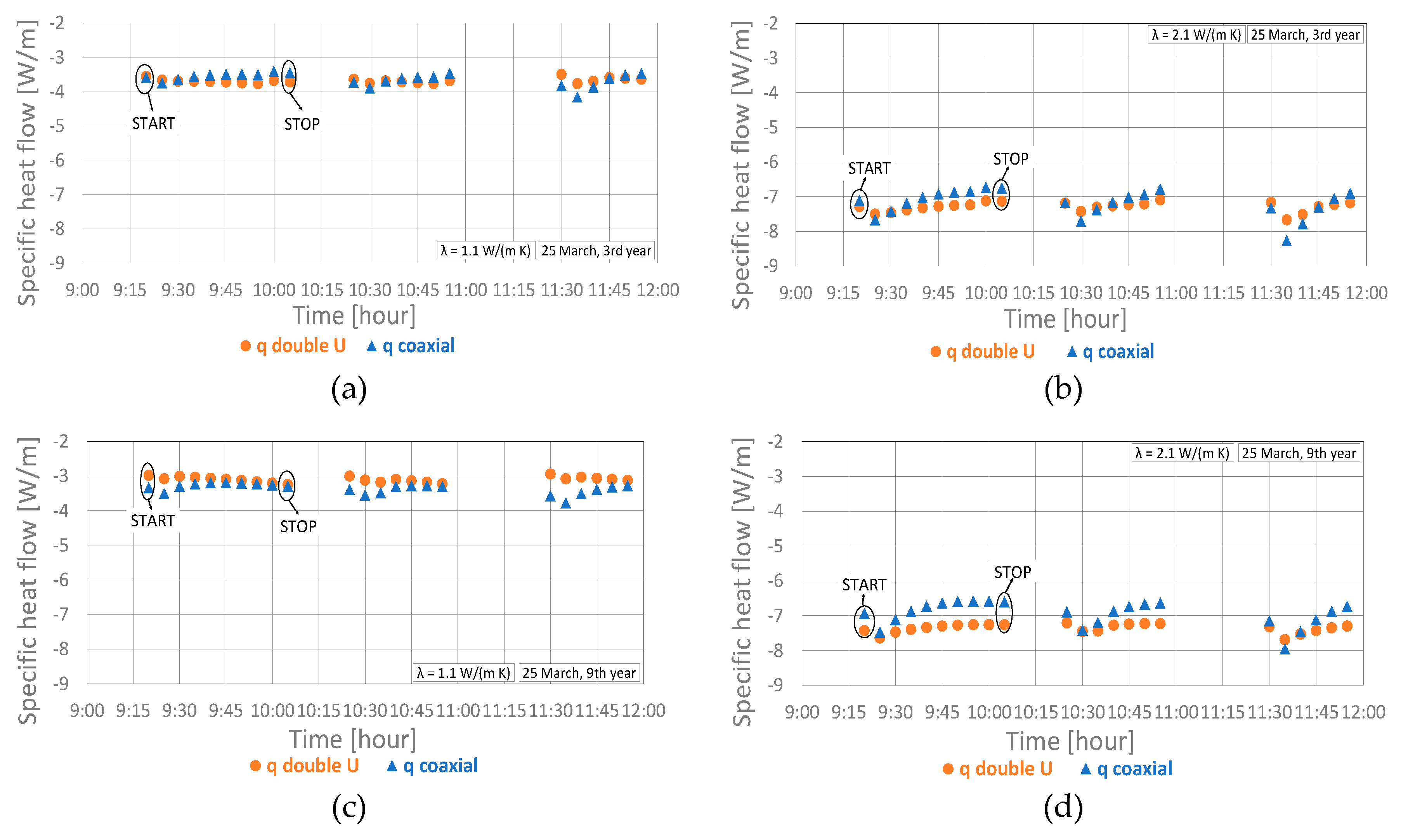
3.2. Short-Term Analysis

The following considerations are also relevant when a dynamic thermal load is applied; therefore, they are useful for explaining the thermal behaviors reported previously in the long-term analysis.

The first three operating hours of the heat pump (from the 744th to the 747th hour of simulation) are shown in Figure 18, and it is possible to divide the diagram into three parts:

(1)

At the start of the heat pump (first period) for the first six time steps (i.e., 30 min), the coaxial borehole heat exchanger is characterized by a higher outlet fluid temperature than that of the double U. This occurs due to the larger fluid volume of the coaxial probe (237 L). As a consequence, the thermal capacitance of its stationary transfer fluid is greater than that of the double U-tube, which has a volume of 168 L. This means that when the heat pump is switched on in the two BHEs, the same inlet fluid temperature solicits two different thermal capacitances (i.e., that of the heat-carrier fluid), and the coaxial probe, which has the greater capacitance, has a higher outlet fluid temperature. The thermal capacitance of the transfer fluid inside the probe is a key parameter for the first 30 minutes. Notably, the coaxial BHE shows a flatter pattern in the first time steps than the double U-tube because the transit time of the entire coaxial probe is longer (17 min vs. 12 min for the double U-tube). To better understand the difference between the performance of the BHEs, the outlet fluid temperatures are plotted against the natural logarithm of time in Figure 18.

(2)

In the second period (from the 30th minute until 1.5 h of operation) the thermal capacitance of the grouting material is the main factor affecting the thermal performance of the BHEs. The double U probe, with a grouting material volume (0.71 m³) greater than that of the coaxial probe (0.27 m³), has a higher outlet fluid temperature in this period.

(3)

In the third period, the thermal behavior of the coaxial borehole heat exchanger is better than that of the double U-tube. This occurs due to its lower borehole thermal resistance R_b of 0.03 (K∙m)/W, which is about half that of the double U-tube.

4. Conclusions

We analyzed the energy performance of two different types of vertical borehole heat exchangers: the double U-tube and the coaxial BHEs, subjected to a balanced thermal load for nine years using the CaRM tool. This detailed model was used to analyze the short-term variations in the thermal behavior of the ground heat exchanger with a dynamic thermal load.

Simulations revealed that the thermal performance of the borehole heat exchangers, when intermittent operating modes of the ground source heat pump system are set, significantly depend on the thermal capacitance of both the heat-carrier fluid and the grouting material and on the thermal resistance of the borehole heat exchanger.

Under equal boundary conditions, the coaxial borehole heat exchanger, due to a larger volume of the probe and a borehole thermal resistance lower than that of the double U-tube, exchanges of 2.9–5.5% more energy in heating mode and 0–1.6% in cooling mode with a ground thermal conductivity of 1.1 W/(m∙K). With a ground thermal conductivity of 2.1 W/(m·K), the rates are 4.3–6.3% in heating period and 5.4–7.3% in cooling. As result, a more conductive ground shows that the coaxial borehole heat exchanger provides better thermal performance.

References

- Oliver, H.; Braud, J. Thermal exchange to earth with concentric well pipes. Trans. ASAE 1981, 24, 906–910. [Google Scholar] [CrossRef]
- Mei, V.C.; Fischer, S.K. Vertical Concentric Tube Ground Couoled Heat Exchangers. ASHRAE Trans. 1983, 89, 391–406. [Google Scholar]
- Hellström, G. Ground Heat Storage, Thermal Analyses of Duct Storage Systems. Ph.D. Thesis, University of Lund, Lund, Sweden, 1991. [Google Scholar]
- Zanchini, E.; Lazzari, S.; Priarone, A. Effects of flow direction and thermal short-circuiting on the performance of small coaxial ground heat exchangers. Renew. Energy 2010, 35, 1255–1265. [Google Scholar] [CrossRef]
- Acuña, J.; Palm, B. Distributed thermal response tests on pipe-in-pipe borehole heat exchangers. Appl. Energy 2013, 109, 312–320. [Google Scholar] [CrossRef]
- Wood, C.J.; Liu, H.; Riffat, S.B. Comparative performance of ‘U-tube’ and ‘coaxial’ loop designs for use with a ground source heat pump. Appl. Therm. Eng. 2012, 37, 190–195. [Google Scholar] [CrossRef]
- Zarrella, A.; Scarpa, M.; de Carli, M. Short time-step performances of coaxial and double U-tube borehole heat exchangers: Modeling and measurements. HVAC R Res. 2011, 17, 959–976. [Google Scholar]
- Raymond, J.; Mercier, S.; Nguyen, L. Designing coaxial ground heat exchangers with a thermally enhanced outer pipe. Geotherm. Energy 2015, 3, 7. [Google Scholar] [CrossRef] [Green Version]
- Aresti, L.; Christodoulides, P.; Florides, G. A review of the design aspects of ground heat exchangers. Renew. Sustain. Energy Rev. 2018, 92, 757–773. [Google Scholar] [CrossRef]
- Conti, P. Dimensionless Maps for the Validity of Analytical Ground Heat Transfer Models for GSHP Applications. Energies 2016, 9, 890. [Google Scholar] [CrossRef]
- Zeng, H.Y.; Diao, N.R.; Fang, Z.H. A Finite Line-Source Model for Boreholes in Geothermal Heat Exchangers. Heat Trans. Asian Res. 2002, 31, 558–567. [Google Scholar] [CrossRef]
- Carslaw, J.C.; Jaeger, H.S. Conduction of Heat in Solids, 2nd ed.; Clarendon Press: Oxford, UK; Oxford University Press: New York, NY, USA, 1959. [Google Scholar]
- Zanchini, E.; Lazzari, S.; Priarone, A. Improving the thermal performance of coaxial borehole heat exchangers. Energy 2010, 35, 657–666. [Google Scholar] [CrossRef]
- Marcotte, D.; Pasquier, P. On the estimation of thermal resistance in borehole thermal conductivity test. Renew. Energy 2008, 33, 2407–2415. [Google Scholar] [CrossRef]
- Pasquier, P. Ghe3d: A 3d Transient Ground Heat Exchanger Numerical Model; Internal Technical Report; Golder Associates: Montreal, QC, Canada, 2007. [Google Scholar]
- Zanchini, E.; Jahanbin, A. Finite-element analysis of the fluid temperature distribution in double U-tube Borehole Heat Exchangers Ground-coupled heat pump systems View project. Artic. J. Phys. Conf. Ser. 2016, 745, 032002. [Google Scholar] [CrossRef]
- Zeng, H.; Diao, N.; Fang, Z. Heat transfer analysis of boreholes in vertical ground heat exchangers. Int. J. Heat Mass Transf. 2003, 46, 4467–4481. [Google Scholar] [CrossRef]
- Zarrella, A.; Scarpa, M.; de Carli, M. Short time step analysis of vertical ground-coupled heat exchangers: The approach of CaRM. Renew. Energy 2011, 36, 2357–2367. [Google Scholar] [CrossRef]
- Cheap-GSHPs. Cheap and Efficient Application of Reliable Ground Source Heat Exchangers and Pumps. Available online: https://cheap-gshp.eu/ (accessed on 17 April 2019).