Single and Multiobjective Optimal Reactive Power Dispatch Based on Hybrid Artificial Physics–Particle Swarm Optimization


1
Energy Systems Research Laboratory, Department of Electrical and Computer Engineering, Florida International University, Miami, FL 33174, USA
2
Department of Electrical and Computer Engineering, Taibah University, Medina 42353, Saudi Arabia
*
Author to whom correspondence should be addressed.
Energies 2019, 12(12), 2333; https://doi.org/10.3390/en12122333
Submission received: 23 April 2019
/
Revised: 10 June 2019
/
Accepted: 10 June 2019
/
Published: 18 June 2019
(This article belongs to the Special Issue Applications of Heuristic Methods to Electrical Power Engineering)
Abstract
:The optimal reactive power dispatch (ORPD) problem represents a noncontinuous, nonlinear, highly constrained optimization problem that has recently attracted wide research investigation. This paper presents a new hybridization technique for solving the ORPD problem based on the integration of particle swarm optimization (PSO) with artificial physics optimization (APO). This hybridized algorithm is tested and verified on the IEEE 30, IEEE 57, and IEEE 118 bus test systems to solve both single and multiobjective ORPD problems, considering three main aspects. These aspects include active power loss minimization, voltage deviation minimization, and voltage stability improvement. The results prove that the algorithm is effective and displays great consistency and robustness in solving both the single and multiobjective functions while improving the convergence performance of the PSO. It also shows superiority when compared with results obtained from previously reported literature for solving the ORPD problem.
1. Introduction
Optimal reactive power dispatch (ORPD) is an important problem in power system operation. The economy of grid operation has two main aspects to consider: active (Watt) and reactive (Var) power control problems. The Watt problem concerns regulating and controlling the output of the generation units to reduce the overall costs of production. On the other hand, the Var is considered a more complex problem due to the nature of control variables involved in its operation, where it focuses on different voltage control aspects of the grid components (i.e., tap-changing transformers, reactive compensators, etc.) to reduce the overall grid losses, and improve voltage balance. ORPD is considered a pivotal problem in this manner, which aims to solve highly constrained, nonconvex, and nonlinear optimization problems that possess both discrete and continuous control variables to achieve important goals, such as minimizing active power losses and voltage deviations, while improving the voltage stability index of the grid. These types of operational issues emerge due to the complexity arising in grid modernization. Specifically, an optimal reactive power dispatch is essential to help maintain the voltage level in loading conditions by reducing the voltage deviation and power quality issues that emerge from the stochastic fluctuations of the power output. The latter due to the unpredictability of sources such as renewable energy and electric vehicle integration.
Recent years have witnessed growing attention on the metaheuristics and population-based techniques to solve various problems in power system operation and control. These modern approaches have been widely recognized to overwhelm the traditional gradient-based optimization methodologies that have been used for a long time [1]. The gradient-based approaches to reactive power planning and operation have many valid drawbacks and criticisms. One is that solving a large number of gradient variables requires intensive computations and tends to converge very slowly [2]. Another aspect of its drawback is that the gradient solution to the objective function is utilized as a search method is based on too many assumptions. for example, the active and reactive power are not directly influenced by voltage levels and phase Angles ϴ [3]. This is unacceptable since ϴ is considered one of the factors that determine the active power loss due to its link to the variation of the real power in the system. Therefore, the inconsistencies in formulating its mathematical representation lack adequate modeling accuracy, leading to repercussions in its search juncture.
On the other hand, metaheuristic approaches allow abstract-level description that provide non-specificity, which is useful for solving a wide range of problems that are presided over by the metaheuristics’ upper-level strategies which influence greater search capabilities. They are based on utilizing search capabilities, mainly embodied as a form of memory, to be re-evaluated by successive iterations to steer their search process. This has helped to rapidly escalate its use in the literature to solve a variety of engineering and scientific-based, real-life problems. Many traditional and bio-inspired optimization algorithms have touched on different aspects of the ORPD problem in the literature, such as genetic algorithms (GA) [4,5], particle swarm optimization (PSO) [6,7,8,9], evolutionary programming (EP) [1,10], Tabu search [11], dynamic programming (DP) [12,13], harmony search optimization (HSO) [14], gravitational search algorithm (GSA) [15,16,17], and grey wolf optimizer (GWO) [18]. Some of these methodologies show superior performance in reaching a near-global optimum while greatly prevailing over the difficulty that arises due to the nonconvexity and nonlinearity nature of such problems.
The significant contribution of this paper is to develop a new hybridization of two naturally-inspired metaheuristics techniques, particle swarm optimization (PSO) and artificial physics optimization (APO), then solve and optimize the complexity and nonlinearity of the ORPD problem and test it on various IEEE test systems to evaluate its search capacity. The PSO is an evolutionary metaheuristic algorithm that imitates the complex social behavior of flocking birds or fish schooling and was firstly introduced by Kennedy and Eberhard [19]. It utilizes a set of potential solutions (known as particles) to explore the search space, where every possible solution (or particle) modifies its position via the learning-by-experience concept from the history of its position and its neighboring particles. The use of PSO, either as a stand-alone or by hybridization with another metaheuristic methodology, has been extensively considered to solve complex problems in various engineering disciplines, including studies related to optimal reactive power dispatch. However, in this paper, we present a new form of hybridization with the APO that has not been applied to the ORPD problem before. The APO is a probabilistic population-influenced algorithm inspired by physics-based swarm intelligence, also known as physicomimetics [20]. In APO, each solution is looked at as an individual that exhibits physical properties such as mass, force, velocity, and position. Derived mainly from Newton’s second law, every particle (solution) can be optimized as the best solution based on the iterative relocations of the population, where a particle’s movement is influenced by the force and inertia of other particles (possible solutions). Recent literature shows the powerful capabilities of APO in solving various kind of problems as a stand-alone algorithm or when hybridized with other algorithms [21,22,23] and it exhibits solid search performance and fast convergence. Hybrid APO–PSO has been used in a previous study to solve dynamic power security analysis [22], but has never been applied to the ORPD problem. Our overall goal is to produce an intact algorithm that combines the global search capabilities of APO with the strong local exploratory search performance of PSO, while improving its convergence characteristics. The APO exhibits flexible and wide-range search features that enhance its global population diversity, adding a powerful searching-mixture when combined with PSO. After building the mathematical representation of each algorithm, we validate the performance of the hybridized algorithm on the IEEE 30, IEEE 57, and IEEE 118 bus test systems, and compare with the results of previously published reports using other methods to verify its capabilities.
This paper is organized as follow. Section 1 presents literature on the metaheuristics methodologies used in power systems and provides insight into the problem. Section 2 provides the mathematical representation and modeling of the ORPD problem. Section 3 describes the mathematical representation and framework for the APO, the PSO, and the hybrid APO–PSO and its application to solve the ORPD problem. Section 4 provides an analysis of the results and compares them with the reported results in the literature. Section 5 concludes the paper and provides suggestions for future studies to be carried out in this area.
2. Mathematical Formulation of the ORPD
The hybrid APOPSO algorithm developed in this work aims to individually and simultaneously minimize three main objectives in the ORPD problem subjected to equality and inequality constraints, namely, minimizing total active power loss, reducing voltage deviations, and improving voltage stability index (the L-index).
2.1. General Optimization Problem Formulation
The general mathematical formulation of an objective function can be expressed as
subject to
where is the objective function to be minimized, E and I are nonlinear constraints represented as vectors that resemble both the independent (control) and dependent variables of the problem. Specifically, x is a vector containing the control variables of the ORPD which namely include the reactive power compensators GC, dynamic tap-setting of transformers T, and voltage levels at generation units Vg. x can be expressed as
y is a vector representing the dependent variables, which include slack generator , voltage levels at transmission lines VL, reactive power from generation units QG, and the apparent power SL. y can be expressed as
2.2. Single Optimization Function Formulation
2.2.1. Minimization of MW Losses Function
The fitness function formulated to reduce the overall MW losses in the system can be expressed as
where NTL is the number of transmission lines in the system, GM is the conductance of the transmission lines between the ith and the jth buses, and is the phase angle between buses i and j.
2.2.2. Minimization of Voltage Deviations
It is highly significant to record and notice all the voltage deviations across all the system’s buses from reference points. This is done to ensure proper consideration of the voltage limits in optimal reactive power planning and operations, and not only as constraints, as bus voltages may operate at their maximum limits without invoking any violation, yet leading to improper reactive power reserves that could cause outages and faults. The fitness function of voltage deviation minimization can be written as
where VLK is the load voltage at the kth load bus, is the desired load voltage at the kth load bus that is usually set to be 1.0 pu, is the reactive power from generators at the kth load bus, is the generator reactive power limit, while NLB and Ng are the number of the load buses and generation units in the system, respectively.
2.2.3. Minimization of Voltage Stability Index
The L-index is utilized in this work as a metric indicator of voltage stability performance. This index is newly introduced and presented in [24]. It assesses the steady-state voltage levels for any node in the test system and provides highly consistent results compared to other voltage stability indices, e.g., voltage collapse prediction index (VCPI), equivalent node voltage collapse index (ENVCI), fast voltage stability index (FASI), etc. [25]. Such indices are crucial factors to be considered in the planning and operation of an electrical network. L-index can be expressed as
such that
where is the number of the PV (generator type) buses in the system.
2.3. System Constraints (Independent and Dependent Variables)
2.3.1. Equality Constraints
Equality constraints of the ORPD are the usual nonlinear power flow equations which provide voltage levels and angles at each node in the test system, expressed as
where PGi and PDi are the real power generation and demand at the system respectively while and are the real and imaginary entries of the bus admittance matrix corresponding with the ith row and jth column, for i = 1, …,
where QGi and QDi are the reactive power generation and demand at the system respectively, for i = 1, .
2.3.2. Inequality Constraints
It should be noted that both dependent and independent variables must operate within specific limits imposed on them to ensure proper operation. Therefore, we carefully consider both equality and inequality constraints in our modeling. The boundary of operation for the independent (control) variables applies to (i) the slack generator output limit, (ii) reactive power limit of the generation units, (iii) the load buses voltage limits, and (iv) the apparent power flow limit. These operational inequalities can be represented as
where Ng, NLB, and NTL are the numbers of generators, load buses, and transmission lines in the system. The dependent variables, such as (i) the generation unit voltage levels, (ii) reactive power compensators, (iii) the position of the tap transformers, are also operationally restricted and limited as follows
where NC and NRT are the numbers of the compensator devices and regulating transformers, respectively.
2.4. Multiobjective Fitness Function
The previous fitness functions are incorporated into a multiobjective optimization function with penalty factors established to consider the dependent variables into the objective function minimization:
where , , and are penalty factors incorporated to enforce the limits on the control variables to avoid any violation to the voltage deviation and stability index levels, assumed in this work to be 100. The limit values are defined as
3. Mathematical Framework of the Metaheuristic Algorithms
A thorough discussion on the APO and PSO algorithms and their hybridization is presented in this section.
3.1. Artificial Physics Optimization (APO)
APO, as a naturally inspired metaheuristic methodology, is well presented in [20,26]. APO is based on the idea that an exerted force may result in either attractive or repulsive aggregation of physical entities (namely the particles or solutions) leading to a movement that represents the search to find local and global optima. Specifically, the process is based on three main observations: initializations, calculation of force, and motion of particles. At the initialization step, particles are sampled stochastically within a multidimensional decision space. The central presumption of APO is based on treating the particles (possible solutions) as physical entities that exhibit mass, position, and velocity, with the mathematical representation of the mass mapped as the fitness function. The mathematical representation of the mass (fitness) function is expressed as follow:
when f(x) € [−, ], then;
Equations (24) and (25) can be mapped into the interval (0, 1) through an elementary transformation function. The mass functions can be rewritten as
where the function f () is the objective function value at the position of the best received value for the individual (swarm particle), while f () refers to the function value of the worst individual swarm reported:
where S = {1; population of N agents}
Once each particle’s mass is identified, a velocity vector will be produced. The inevitable changes in velocity in the iteration process are controlled by the level and amount of force exerted on the particle, which is the second stage of the algorithm; calculation of the force, which is based on the mass of the particle and its distance from its neighbors. The force exerted on a particle i via another particle j can be found via:
where is the kth force quantity enforced on particle i via particle j in their dimensions; and are the kth dimension coordinates for the swarm particles i and j; is the distance between these coordinates. Sgn(r) represents the signum function, while G(r) denotes the gravitational factor that follow the changes iteratively with . Both of them can be expressed as:
The g can be assumed as any value to provide simplicity and flexibility when experimenting. In our studies, we assumed these values based on studies presented in [25]. The total force exerted on all particles can be rewritten mathematically as:
The third stage is understanding the motion principles of the particles in the decision space, where the computed force is utilized to determine the velocity of the particles that are used to find (and then update iteratively) the respective positions of the particles. Such motions are set in either two- or three-dimensional space, in which particles can be locally spotted, and can be mathematically represented as
where and are the kth components of particle i’s velocity and distance at iteration t. Beta is a uniformly distributed random number distributed on the interval (0, 1), while w is the user-specified inertia weight that can be iteratively updated, usually between 0.1 to 0.99. The inertia influences how two velocity values iteratively change. Larger values of w is a good indication of greater velocity changes, while small values is only used when we only want to facilitate a local search. Each particle identifies the information of its neighbors, while the physical attractiveness/repulsiveness rule serves as the search strategy in this algorithm to guide the population to search within the region of a possible solution in accordance with their fitness function. The high accuracy and ability to map the particle’s mass as a fitness function influence the whole optimization process, to which the relationship is proportionally related; the more accurately the objective function is designed, the bigger mass will be produced, which leads to a higher level of attractiveness, or in other words, more optimized searching strength, as particles will be naturally attracted to higher masses.
The iteration process in the APO leads to the updating of all particles’ positions, and accordingly, the objective fitness function is adjusted to those new positions. Then, the fitness function identifies a new best individual and marks its position vector as the best solution. In this way, the second and third steps of the algorithm, force calculation and motion, are iteratively performed until a stopping criterion is achieved. Such criteria may be a predetermined number of executed iterations or reaching several successive iterations with no difference in the value of the best obtained particle position.
3.2. Particle Swarm Optimization (PSO)
PSO is a population-based, bio-inspired metaheuristic algorithm that was established by Kennedy and Eberhart in 1995 [19]. It is based on the concept of evolutionary computational method, where a system of study is started with an initial population of randomized solutions, updated iteratively in the process of searching for the local and global optima. The candidate solutions, known as particles, fly in the decision space with the velocity obtained in its previous best solutions, as well as its group’s best results. Both the velocity and position of each particle are updated accordingly using the following mathematical formulas:
where (t) and (t) are vector representations in the solution space for both the velocity and position of particle i, while Pbest and gbest are the best individual and global optimal obtained solutions. The performance of PSO as a validated and well-proven metaheuristic technique is widely spread in the literature in different fields of study. This is due to its powerful searching capacity and premature convergence without the need to find local optimal. Figure 1 shows the basic concept of the searching methodology and motion principle for particle i in PSO, where V(t), Xm, and X are three vectors describing the coordinates of the best solution in the decision space.
3.3. Hybridization of APO and PSO to Solve the ORPD Problem
The primary goal of establishing a hybridization of APO and PSO is to combine their individual strengths to form an optimized algorithm that utilizes the global search capabilities of APO with the strong local exploratory search performance of PSO, while improving its convergence performance. In other words, such hybridization aims to form a successful partnership among the local and global searching capabilities of the two algorithms to overcome any shortages each one may face if performed alone. Talbi et al. (2009) provide extensive analysis of the concept of integrating two metaheuristic techniques, which can be achieved on either lowly or highly heterogeneous integration [27,28]. This work combines the two algorithms as a low-heterogeneity routine. Successful implementation of the hybridization requires modifying the particles’ velocity and position equations, as follows:
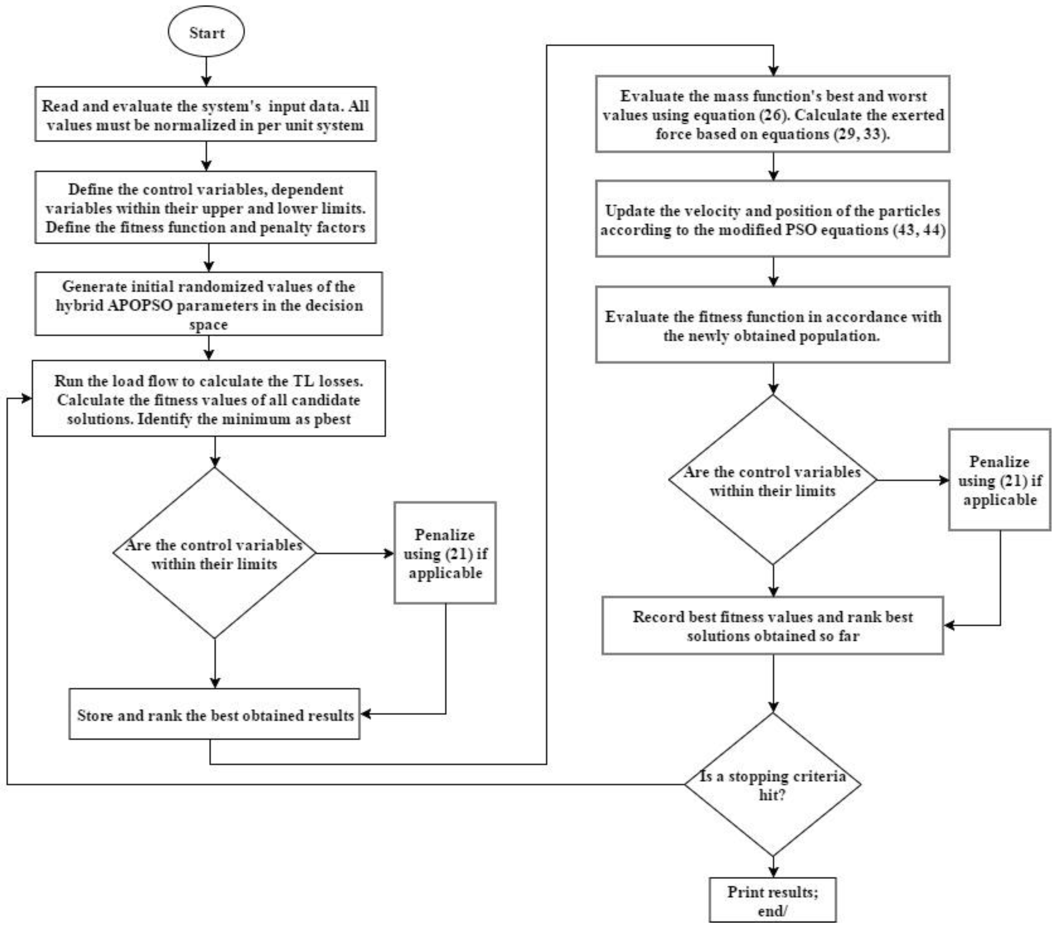
In our proposed APOPSO to solve the ORPD, we first define the dependent and control variables with their respective limits over a defined fitness function. Then, we randomly initialize the input values of the population (particles or swarms). Each particle represents a candidate solution. After the initialization step, we establish the best and worst values of the load flow and rank the obtained results. After that, the mass function given in Equation (26) will be assessed according to those results, and a force calculated using Equations (29) and (33) will be exerted on the particles, then their velocity and positions are updated based on Equations (36) and (37) and the distance between them according to (30), then ranking the newly produced results according to their fitness values. The process is repeated iteratively, and in each iteration we check whether there is a violation that occurred at any level to ensure proper operation within the limits. The iteration process stops updating the velocities and positions once an ending criterion is met. Figure 2 shows the flowchart of the proposed APOPSO algorithm. The pseudocode of the combined algorithm is as follows:
Step 1: Read and evaluate the input data [Tr, Qc, ….]. All values must be normalized in per unit system.
Step 2: 2.1: Define the independent (control) variables X within their specific boundary levels; 2.2: Define the dependent variables Y within their specific boundary levels; 2.3: Define the fitness function with its associated penalty factors.
Step 3: Generate an initial randomized population with N agents in the decision space. Specify the desired number of iterations to be performed. It should be noted that the initial positions of the population must be strictly within their boundary levels.
The initialized value of the kth control parameter in an ith particle (candidate solution) can be found using the following mathematical expression:
Rand is a number randomly allocated in the interval [0–1], while and are the boundary limits of the control variable d. The ith particles corresponding to the optimal dispatch problem can be rearranged in a vector form as follows:
At i = 1, 2, ……, N.
Step 4: Run the system’s load flow to calculate the transmission line losses. Calculate the fitness values of all candidate solutions using the mass function. Select the minimally obtained result as best.
Step 5: Check if the control variables are within their boundary limits. If yes, proceed to step 6. If no, then penalize using the penalty function in Equation (21). The penalization is considered only for the multiobjective case studies.
Step 6: Evaluate the mass function’s best and worst values using Equation (26). Calculate the force based on as in Equation (33).
Step 7: Update the velocity and position of the particles according to the modified PSO Equations (38) and (39).
Step 8: Evaluate the fitness function by newly obtained population information. Check if the control variables are within their boundary limits. If yes, proceed to Step 9. If no, then penalize using the quadratic penalty function in Equation (21).
Step 9: Record the best fitness values and rank the best obtained solutions.
Step 10: Repeat Steps 4–9 until a stopping criterion is achieved.
Step 11: Print best results and end.
4. Simulation and Results
This section provides an analysis of the obtained results on the three (IEEE 30, IEEE 57, and IEEE 118) test systems to verify the capacity of the proposed algorithm to solve the ORPD problem. Table 1 shows the parameters of the test systems used in our study. The test system’s detailed line data and parameters can be found in [29,30,31]. The results were obtained utilizing a developed Matlab code that was run in an i7 Core, 3 GHz, 16 GB RAM computer with Matlab 2018-b. For each test system, the main outcomes to be recorded is the influence of the algorithm on the minimization of the MW losses, the minimization of the voltage deviation, and the voltage stability index (VSI) improvement (L-index), first individually and then concurrently. We implemented the APOPSO algorithm on a total population of 200 particles, with a maximum iteration run of 100.
4.1. IEEE 30 Bus Test System
The IEEE 30-bus test system has a total of six synchronous generators located at buses 1 (the slack bus), 2, 5, 8, 11, and 13, 41 transmission lines, four power transformers with off-nominal tap-settings at lines 6–9, 6–10, 4–12, and 28–27, and nine reactive power compensators at buses 10, 12, 15, 17, 20, 21, 23, 24, and 29, respectively. This test system has a total active and reactive consumption of 2.834 and 1.262 per unit on a 100-MVA base. It has a total of 19 control variables that we considered in our study: six generator voltage inputs, four transformers tap-settings, and nine reactive power compensation devices. For this study to be precise, we constrained the level of the system’s voltages to be strictly within limits of 0.95 and 1.10 p.u. The lower and upper limits of the transformer’s tap settings are set to be between 0.9 and 1.1 p.u., whereas the reactive compensation devices should be ranged from 0 to 5 MVAR. Failure for a result to be within these limits will result in the use of the penalty factors we introduced in the multiobjective fitness function in Equation (21). The test system data was obtained from [29].
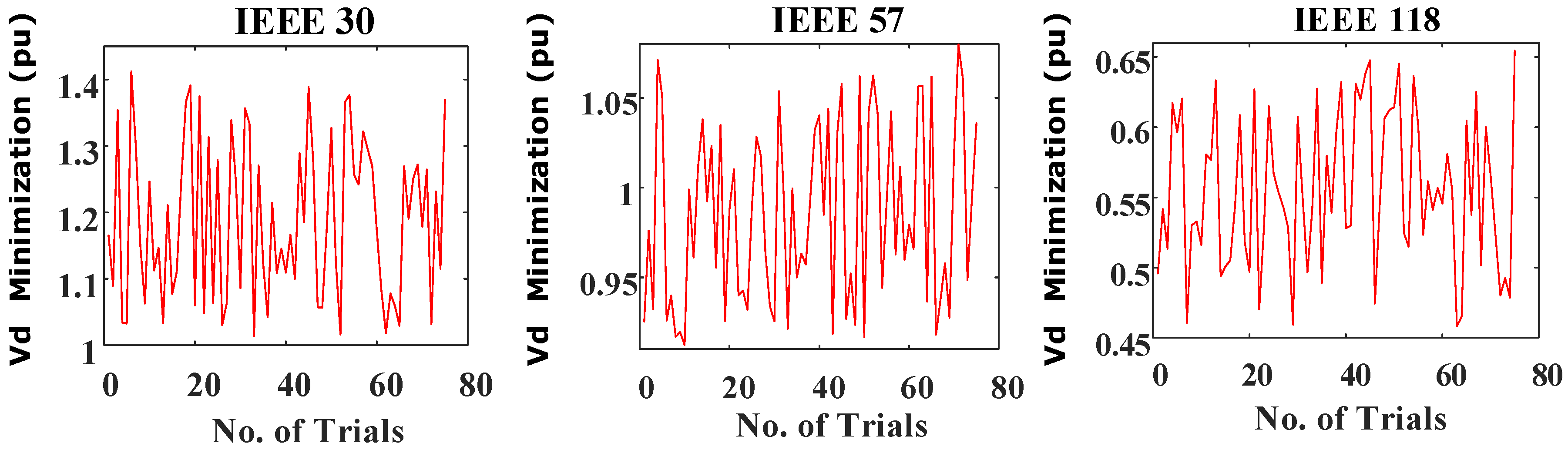
We measure the strength of our proposed algorithm by initially investigating each targeted objective (loss minimization, Vd minimization, and VSI improvement) individually. Table 2 shows the results obtained for the hybrid APOPSO when applied on the IEEE 30 bus system. The table illustrates the results when the simulation performed via APO and PSO separately at first before their hybridization. The results show great robustness over their integration throughout 100 consecutive trials. The initial values were proposed from previous literature conducted on the same test system, yet for different studies [32,33,34]. The optimal results obtained are then compared with previous findings reported in the literature in an attempt to illustrate the high consistency and power of the APOPSO algorithm. Table 3 presents the values for the three obtained objectives in comparison with other results reported by differential evolution algorithm (DE) [10], gravitational search algorithm (GSA) [15], particle swarm optimization with agent leader algorithm (ALCPSO) [8], and comprehensive learning particle swarm optimization (CLPSO) [35] in regard to the control variables of this study. The results show the superiority of the APOPSO algorithm over the reported results from these studies. For example, the power flow results in [8,15] specify values that are not considered optimal at some buses in the system. For instance, reactive power outputs from compensators at buses 15, 17, 20, 21, and 23 are either at or near the violation of their minimum limits, where they are too small to be operationally feasible, compared with the values obtained in DE, CLPSO, and APOPSO. The overall findings for each case study considered demonstrate APOPSO to be superior to the reported algorithms. The final values at 100, 80, and 50 trials, respectively, for a population of 200 objects are as follow: Ploss = 4.3982 MW; Vd = 1.0477; L-index = 0.1267. Table 4 shows the statistical analysis of our simulation, with the best, worst, mean, and standard deviations over 100 trials. Figure 3 illustrates the Vd throughout these trials for the three test systems. The convergence performance of the PSO significantly improved with the hybridization, and Figure 4 shows the algorithm’s fast convergence characteristic towards the optimal results considering the loss minimization case on the IEEE 30 bus system, while Figure 5 provides an insight into the statistical accuracy of the algorithm, presenting the Weibull distribution of the VSI values in 100 trials around the mean value.
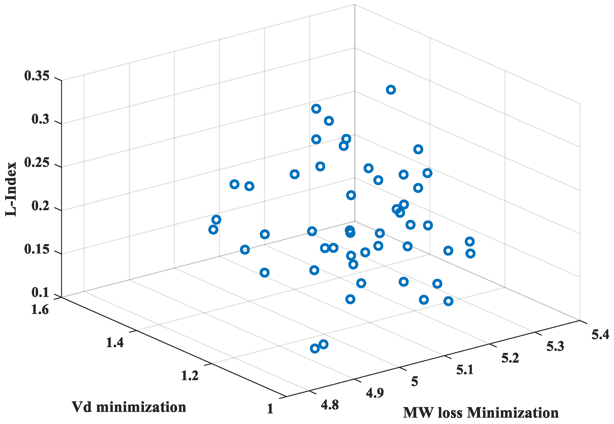
The multiobjective values obtained for MW loss, voltage deviation and L-index are simultaneously shown in the rightmost column in Table 3, whereas Figure 6 depicts the produced Pareto optimal values for the multiobjective fitness function on the IEEE 30 test system. In addition to its superiority compared in the reported literature, the results obtained from APOPSO show no violations at any dependent variables in the system. It should be mentioned that we considered the nondomination criteria in the sorting and crowding of the distances when it comes to solving the multiobjective equation. Specifically, fuzzification of each fitness function incorporated in Equation (21) and applied on particle Z can be carried according to:
where the maximum and minimum limits correspond to the objective function of the ith objective function, respectively. The normalization of contribution from each fitness function on particle Z can be calculated as:
where R is the number of nondominated obtained results, and N is the total number of fitness (objective) functions.
4.2. IEEE 57 Bus Test System
The IEEE 57-bus system consists of seven synchronous generators located at buses 1, 2, 3, 6, 8, 9, and 12, 80 transmission lines, three reactive power compensators located at buses 18, 25, and 53, and 15 transformers with off-nominal tap ratio. Line data, bus data, variable limits, and the initial values of the control variables are given in [30,31]. Twenty-five variables are set within the decision space to be investigated using the APOPSO algorithm, which are seven generator voltages, three reactive compensators, and 15 power transformers’ tap-settings. Details about the tests system parameters are shown in Table 1. Table 5 presents the values obtained when applying the APOPSO algorithm on the IEEE 57 test system. It also shows the multiobjective results in the rightmost column when implementing the algorithm over the defined multi-objective function MOF function in Equation (21) to solve for the three cases with defined penalties for violation of the limits. It shows the capacity of APOPSO to efficiently optimize nonlinear, constrained problems in complex systems.
As the results show, APOPSO demonstrates greater search capabilities in finer results obtained compared with GSA [15], multiobjective differential evolution algorithm (MODE) [36], and chaotic krill herd optimization (CKHA) [37]. Further comparisons show the dominance of APOPSO over other reported findings that are not presented for simplicity of presentation. Table 4 shows the statistical analysis of the obtained results for the IEEE 57 test system over 100, 75, and 50 trials for MW loss minimization, Vd minimization, and voltage stability improvement respectively. While Figure 3 plots the Vd minimization values obtained over the trials, Figure 7 presents the Pareto optimal obtained for the IEEE 57 test system. The eminence search capabilities of the APOPSO is perfectly illustrated in the Weibull distribution presented in Figure 5, which shows the precision of the algorithm to determine the optimum values around the mean obtained over 50 trials.
4.3. IEEE 118 Bus Test System
For us to confirm the capacity performance and robustness of the proposed APOPSO algorithm for solving the ORPD problem on a large scale, we applied it on the IEEE 118 test system. This system’s line data and parameters were adopted from [31]. It has 54 synchronous generator-buses, 64 load-buses, 12 reactive power compensators, nine tap-setting power transformers, and 186 transmission lines. The bus voltages levels are constrained to remain within the strict boundary of the per unit range [0.95, 1.1]. Details of the test system’s parameters are shown in Table 1. The table presents the values of the simulation results on the IEEE 118 test system.
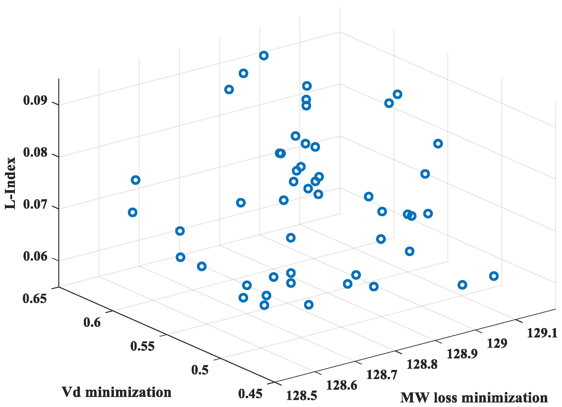
The results for the multiobjective function in Equation (21) after its fuzzification are presented in the rightmost column of the table, and its Pareto optimal is shown in Figure 8. The results present evidence of the strength and robustness of APOPSO in solving real-life, highly complex scenarios, as the produced outcomes show good optimization for the highly-constrained, nonlinear, multiobjective fitness function in a large complex system like the IEEE 118. Table 4 presents the statistical analysis of the simulation process for each objective, while Table 6 shows the results obtained for each fitness function when simulated individually and simultaneously. No violations have been recorded in the dependent variables throughout the study. Figure 9 presents an illustration of the range of values obtained over the 100 trials for the MW loss reduction objective for this test system. The results show superior consistency in getting the results within a close range over a large number of iterations.
5. Conclusions
A new hybrid technique for solving the ORPD problem was established in this paper. The proposed APOPSO algorithm was tested and verified on three IEEE test systems: the 30, 57, and 118 bus systems. The results demonstrated the excellent search capacity of the PSO and APO algorithms when they are integrated. This process creates a robust hybrid algorithm to solve the ORPD optimization problem. Furthermore, the consistency of the optimized results in large complex systems such as the IEEE 57 and 118 bus systems prove that the combined algorithm overcomes some of the difficulties the PSO traditionally faces. For instance, being trapped in local optima, which usually lead to slower convergence. Comparison with previously reported ORPD results based on different metaheuristic methodologies verified the obtained results of the APOPSO algorithm, which shows superiority in most of the obtained results for MW loss minimization, voltage deviations minimization, and voltage stability improvement. The results obtained were based on the solution of both single and multiobjective fitness functions. The results of the hybrid algorithm produced no violations of any of the constraints placed on the dependent variables. Overall, the APOPSO algorithm shows great potential for various types of studies. Future studies may include the incorporation of electric vehicles to improve the voltage profiles’ test system during specific operation criteria of the ORPD problem. The results of [38,39,40] could be used for such a study. Another aspect to investigate is the integration of flywheel energy storage systems (FESS) in the ORPD problem when integrated into the grid [41].
Author Contributions
Conceptualization, A.T. and E.A.; Methodology, A.T. and E.A. Software, A.T. and E.A.; Validation, A.T. and E.A. and M.O.A.; Formal Analysis, A.T.; Investigation, A.T.; Resources, A.T.; Data Curation, A.T.; Writing-Original Draft Preparation, A.T.; Writing-Review & Editing, A.T. and E.A. and M.O.A.; Visualization, E.A.; Supervision, M.O.A.; Project Administration, M.O.A.; Funding Acquisition, A.T.
Funding
This research received no external funding.
Conflicts of Interest
The authors declare no conflict of interest.
Glossary
| ORPD | Optimal Reactive Power Dispatch |
| PSO | Particle Swarm Optimization |
| APO | Artificial Physics Optimization |
| APOPSO | Artificial Physics-Particle Swarm Optimization |
| OPF | Optimal Power Flow |
| GA | Genetic Algorithm |
| EP | Evolutionary Programming |
| GSA | Gravitational Search Algorithm |
| DE | Differential Evolution Algorithm |
| HSO | Harmony Search Optimization |
| DP | Dynamic Programming |
| GWO | Grey Wolf Optimizer |
| ALCPSO | Particle Swarm Optimization with Agent Leader Algorithm |
| CLPSO | Comprehensive Learning Particle Swarm Optimization |
| MODE | Multiobjective Differential Evolution |
| CKHA | Chaotic Krill Herd Algorithm |
| MW | Mega Watt |
| MV | Mega Volt Ampere |
| PU | Per Unit |
| OF | Objective Function |
| VD | Voltage Deviation |
| VSI | Voltage Stability Improvement |
| Gc | Reactive Power Compensator Devices |
| T | Tap-setting of Transformers |
| Vg | Voltage levels at the generation units |
| PGSlack | The Slack Generator |
| VL | Voltage levels at the transmission lines |
| QG | Reactive Power from Generation Units |
| SL | Apparent Power at the System |
| NC | Number of the compensator devices |
| NRT | Number of the regulating transformers |
| Ng | Number of the generation units in the system |
| NLB | Number of the load buses in the system |
| NTL | Number of the transmission lines in the system |
| The number of the PV (generator type) buses | |
| The kth force quantity enforced on particle i via particle j in their dimensions | |
| The total force exerted on all particles | |
| The kth component of particle i ’s velocity at iteration t | |
| The kth component of particle i ’s distance at iteration t | |
| The normalization (fuzzification) factor from each fitness function on particle Z | |
| Pbest | Individual swarm’s best local solution |
| gbest | Best global obtained solution |
| VLK | The load voltage at the kth load bus |
| The desired load voltage at the kth load bus | |
| GM | The conductance of the transmission lines between the ith and the jth buses |
| The phase angle between buses i and j |
References
- Wu, Q.H.; Ma, J.T. Power system optimal reactive power dispatch using evolutionary programming. IEEE Trans. Power Syst. 1995, 10, 1243–1249. [Google Scholar] [CrossRef]
- Belegundu, A.D.; Chandrupatla, T.R. Optimization Concepts and Applications in Engineering; Chapter 3; Prentice Hall: Upper Saddle River, NJ, USA, 1999. [Google Scholar]
- Shoults, R.R.; Sun, D.T. Optimal power flow based upon P-Q decomposition. IEEE Trans. Power Appar. Syst. 1982, 101, 397–405. [Google Scholar] [CrossRef]
- Chen, C.R.; Lee, H.S.; Tsai, W. Optimal Reactive Power Planning Using Genetic Algorithm. In Proceedings of the IEEE International Conference on Systems, Man and Cybernetics, Taipei, Taiwan, 8–11 October 2006; Volume 6, pp. 5275–5279. [Google Scholar]
- Subbaraj, P.; Rajnarayanan, P.N. Optimal reactive power dispatch using self-adaptive real coded genetic algorithm. Electr. Power Syst. Res. 2009, 79, 374–381. [Google Scholar] [CrossRef]
- Le, D.A.; Vo, D.N. Optimal reactive power dispatch by pseudo-gradient guided patiicle swarm optimization. In Proceedings of the 2012 10th International Power & Energy Conference (IPEC), Ho Chi Minh City, Vietnam, 12–14 December 2012; pp. 7–12. [Google Scholar]
- Yoshida, H.; Kawata, K.; Fukuyama, Y.; Takayama, S.; Nakanishi, Y. A particle swarm optimization for reactive power and voltage control considering voltage security assessment. IEEE Trans. Power Syst. 2000, 15, 1232–1239. [Google Scholar] [CrossRef]
- Singh, R.P.; Mukherjee, V.; Ghosal, S.P. Optimal reactive power dispatch by particle swarm optimization with an aging leader and challengers. Appl. Soft Comput. 2015, 2, 298–309. [Google Scholar] [CrossRef]
- Liu, Z.F.; Ge, S.Y.; Yu, Y.X. Optimal reactive power dispatch using chaotic particle swarm optimization algorithm. Dianli Xitong Zidonghua (Autom. Electr. Power Syst.) 2005, 29, 53–57. [Google Scholar]
- El Ela, A.A.; Abido, M.A.; Spea, S.R. Differential evolution algorithm for optimal reactive power dispatch. Electr. Power Syst. Res. 2011, 81, 458–464. [Google Scholar] [CrossRef]
- Yutian, L.; Li, M. Reactive Power Optimization based on Tabu Search Approach. Autom. Electr. Power Syst. 2000. Available online: http://en.cnki.com.cn/Article_en/CJFDTOTAL-DLXT200002014.htm (accessed on 28 March 2019).
- Lu, F.C.; Hsu, Y.Y. Reactive power/voltage control in a distribution substation using dynamic programming. IEE Proc. Gener. Transm. Distrib. 1995, 142, 639–645. [Google Scholar] [CrossRef] [Green Version]
- Lu, F.C.; Hsu, Y.Y. Fuzzy dynamic programming approach to reactive power/voltage control in a distribution substation. IEEE Trans. Power Syst. 1997, 12, 681–688. [Google Scholar]
- Khazali, A.H.; Kalantar, M. Optimal reactive power dispatch based on harmony search algorithm. Int. J. Electr. Power Energy Syst. 2011, 33, 684–692. [Google Scholar] [CrossRef]
- Duman, S.; Sönmez, Y.; Güvenç, U.; Yörükeren, N. Optimal reactive power dispatch using a gravitational search algorithm. IET Gener. Transm. Distrib. 2012, 6, 563–576. [Google Scholar] [CrossRef]
- Niknam, T.; Narimani, M.R.; Azizipanah-Abarghooee, R.; Bahmani-Firouzi, B. Multi objective optimal reactive power dispatch and voltage control: A new opposition-based self-adaptive modified gravitational search algorithm. IEEE Syst. J. 2013, 7, 742–753. [Google Scholar] [CrossRef]
- Roy, P.K.; Mandal, B.; Bhattacharya, K. Gravitational search algorithm based optimal reactive power dispatch for voltage stability enhancement. Electr. Power Compon. Syst. 2012, 40, 956–976. [Google Scholar] [CrossRef]
- Sulaiman, M.H.; Mustaffa, Z.; Mohamed, M.R.; Aliman, O. Using the gray wolf optimizer for solving optimal reactive power dispatch problem. Appl. Soft Comput. 2015, 32, 286–292. [Google Scholar] [CrossRef] [Green Version]
- Kennedy, J.; Eberhart, R. Particle Swarm Optimization. In Proceedings of the IEEE International Conference on Neural Networks, Perth, WA, Australia, 27 November–1 December 1995; pp. 1942–1948. [Google Scholar] [CrossRef]
- Spears, W.M.; Gordon, D.F. Using artificial physics to control agents. In Proceedings of the 1999 International Conference on Information Intelligence and Systems (Cat. No. PR00446), Bethesda, MD, USA, 31 October–3 November 1999; pp. 281–288. [Google Scholar]
- Zhan, X.; Xiang, T.; Chen, H.; Zhou, B.; Yang, Z. Vulnerability assessment and reconfiguration of microgrid through search vector artificial physics optimization algorithm. Int. J. Electr. Power Energy Syst. 2014, 62, 679–688. [Google Scholar] [CrossRef]
- Teeparthi, K.; Kumar, D.V. Multi-objective hybrid PSO-APO algorithm-based security constrained optimal power flow with wind and thermal generators. Eng. Sci. Technol. Int. J. 2017, 20, 411–426. [Google Scholar] [CrossRef]
- Teeparthi, K.; Kumar, D.V. Dynamic Power System Security Analysis Using a Hybrid PSO-APO Algorithm. Eng. Technol. Appl. Sci. Res. 2017, 7, 2124–2131. [Google Scholar]
- Huang, G.M.; Nair, N.K.C. Detection of dynamic voltage collapse. IEEE Power Eng. Soc. Summer Meet. 2002, 3, 1284–1289. [Google Scholar]
- Durairaj, S.; Kannan, P.S. Improved genetic algorithm approach for multi-objective contingency constrained reactive power planning. In Proceedings of the 2005 Annual IEEE India Conference-Indicon, Chennai, India, 11–13 December 2005; pp. 510–515. [Google Scholar]
- Xie, L.; Zeng, J.; Cui, Z. General framework of artificial physics optimization algorithm. In Proceedings of the 2009 World Congress on Nature & Biologically Inspired Computing (NaBIC), Coimbatore, India, 9–11 December 2009; pp. 1321–1326. [Google Scholar]
- Talbi, E.G. Metaheuristics: From Design to Implementation; John Wiley & Sons: Hoboken, NJ, USA, 2009; Volume 74. [Google Scholar]
- Talbi, E.G. A taxonomy of hybrid metaheuristics. J. Heuristics 2002, 8, 541–564. [Google Scholar] [CrossRef]
- Illinois Center for a Smarter Electric Grid (ICSEG). Available online: https://icseg.iti.illinois.edu/ieee-30-bus-system/ (accessed on 25 February 2019).
- The IEEE 57-Bus Test System. Illinois Center for a Smarter Electric Grid (ICSEG). Available online: https://icseg.iti.illinois.edu/ieee-57-bus-system/ (accessed on 25 February 2019).
- The IEEE 118-Bus Test System. Available online: http://labs.ece.uw.edu/pstca/pf118/pg_tca118bus.htm (accessed on 25 February 2019).
- Lee, K.Y.; Park, Y.M.; Ortiz, J.L. Optimal real and reactive power dispatch. Electr. Power Syst. Res. 1984, 7, 201–212. [Google Scholar] [CrossRef]
- Lee, K.Y.; Park, Y.M.; Ortiz, J.L. A united approach to optimal real and reactive power dispatch. IEEE Trans. Power Appar. Syst. 1985, 104, 1147–1153. [Google Scholar] [CrossRef]
- Ayan, K.; Kılıc, U. Artificial bee colony algorithm solution for optimal reactive power flow. Appl. Soft Comput. 2012, 12, 1477–1482. [Google Scholar] [CrossRef]
- Mahadevan, K.; Kannan, P.S. Comprehensive learning particle swarm optimization for reactive power dispatch. Appl. Soft Comput. 2010, 10, 641–652. [Google Scholar] [CrossRef]
- Basu, M. Multi-objective optimal reactive power dispatch using multi-objective differential evolution. Int. J. Electr. Power Energy Syst. 2010, 82, 213–224. [Google Scholar] [CrossRef]
- Mukherjee, A.; Mukherjee, V. Solution of optimal reactive power dispatch by chaotic krill herd algorithm. IET Gener. Transm. Distrib. 2015, 9, 2351–2362. [Google Scholar] [CrossRef]
- Aljohani, T.; Beshir, M. Distribution System Reliability Analysis for Smart Grid Applications. Smart Grid Renew. Energy 2017, 8, 240–251. [Google Scholar] [CrossRef] [Green Version]
- Aljohani, T.; Beshir, M. Matlab Code to Assess the Reliability of the Smart Power Distribution System Using Monte Carlo Simulation. J. Power Energy Eng. 2017, 5, 30–44. [Google Scholar] [CrossRef] [Green Version]
- Aljohani, T.; Mohammed, O. Modeling the Impact of the Vehicle-to-Grid Services on the Hourly Operation of the Power Distribution Grid. Designs 2018, 2, 55. [Google Scholar] [CrossRef]
- Aljohani, T.M. The flywheel energy storage system: A conceptual study, design, and applications in modern power systems. Int. J. Electr. Energy 2014, 2, 146–153. [Google Scholar] [CrossRef]
Figure 1.
Criteria of the searching in the particle swarm optimization (PSO).

Figure 2.
The proposed algorithm to solve the optimal reactive power dispatch (ORPD) problem.

Figure 3.
The obtained results of voltage deviation (Vd) for 80 trials.

Figure 4.
Convergence performance of the proposed algorithm on the IEEE 30 test system.

Figure 5.
The Weibull distribution of the obtained voltage stability improvement (VSI) values around the mean in 50 trials.
Figure 5.
The Weibull distribution of the obtained voltage stability improvement (VSI) values around the mean in 50 trials.

Figure 6.
Pareto optimal front for the IEEE 30 test system.

Figure 7.
Pareto optimal front for the IEEE 57 test system.

Figure 8.
Pareto optimal front for the IEEE 118 test system.

Figure 9.
Megawatt (MW) loss minimization for the IEEE 118 test system over 100 trials.


Table 1.
The test system’s main parameters.
| Description | IEEE 30 | IEEE 57 | IEEE 118 |
|---|---|---|---|
| Buses, NB | 30 | 57 | 118 |
| Generators, NG | 6 | 7 | 54 |
| Transformers, NT | 4 | 15 | 9 |
| Shunts, NQ | 9 | 3 | 14 |
| Branches, NE | 41 | 80 | 186 |
| Equality constraints | 60 | 114 | 236 |
| Inequality constraints | 125 | 245 | 572 |
| Control variables | 19 | 27 | 77 |
| Discrete variables | 6 | 20 | 21 |
| The base case for Ploss, MW | 5.66 | 27.8637 | 132.45 |
| Base case for VD, pu | 0.58217 | 1.23358 | 1.439337 |
Table 2.
Results obtained for the proposed algorithm on the IEEE 30 bus test system.
| Variables | Initial Values | MW Loss Minimization | Vd Minimization | Voltage Stability Improvement | ||||||
|---|---|---|---|---|---|---|---|---|---|---|
| APO | PSO | APOPSO | APO | PSO | APOPSO | APO | PSO | APOPSO | ||
| VG1 | 1.04 | 1.1000 | 1.1000 | 1.100 | 1.0211 | 1.0299 | 1.012 | 1.0922 | 1.0679 | 1.044 |
| VG2 | 1.05 | 1.1200 | 1.0844 | 1.084 | 1.0110 | 1.0390 | 1.001 | 1.0992 | 1.074 | 1.061 |
| VG5 | 1.01 | 1.0710 | 1.0748 | 1.056 | 1.0180 | 1.0110 | 1.014 | 1.0988 | 1.068 | 1.061 |
| VG8 | 1.01 | 1.0772 | 1.0768 | 1.076 | 0.9981 | 1.0522 | 1.009 | 1.0991 | 1.0799 | 1.057 |
| VG11 | 1.05 | 1.1400 | 1.1310 | 1.091 | 1.0411 | 0.9854 | 0.954 | 1.0987 | 1.0699 | 1.048 |
| VG13 | 1.05 | 1.1430 | 1.1100 | 1.100 | 0.9814 | 0.9910 | 1.000 | 1.098 | 1.091 | 1.089 |
| QC10 (MVAr) | 0 | 5.0000 | 3.5717 | 5.000 | 4.9652 | 1.9754 | 4.102 | 0.0019 | 0.0411 | 0.040 |
| QC12 (MVAr) | 0 | 5.0000 | 3.0984 | 5.000 | 0.0000 | 0.4245 | 2.124 | 0.0255 | 0.0422 | 0.039 |
| QC15 (MVAr) | 0 | 5.0000 | 3.2925 | 4.879 | 4.9681 | 2.2103 | 4.512 | 0.0004 | 0.0413 | 0.038 |
| QC17 (MVAr) | 0 | 5.0000 | 4.0166 | 4.976 | 4.9967 | 2.8845 | 0.000 | 0.0001 | 0.0462 | 0.040 |
| QC20 (MVAr) | 0 | 3.4130 | 3.0309 | 3.821 | 4.8456 | 4.0412 | 5.000 | 0 | 0.049 | 0.037 |
| QC21 (MVAr) | 0 | 5.0000 | 4.0339 | 4.541 | 4.8745 | 3.2412 | 5.000 | 0.0001 | 0.018 | 0.009 |
| QC23 (MVAr) | 0 | 5.0000 | 2.9874 | 2.354 | 4.9964 | 2.4120 | 5.000 | 0 | 0.0191 | 0.019 |
| QC24 (MVAr) | 0 | 5.0000 | 4.3100 | 4.654 | 4.9974 | 2.6612 | 5.000 | 0.007 | 0.04 | 0.010 |
| QC29 (MVAr) | 0 | 2.2233 | 2.7120 | 2.175 | 4.9781 | 2.8456 | 4.120 | 0 | 0.0014 | 0.0011 |
| T11 (6–9) | 1.080 | 1.0377 | 1.0320 | 1.029 | 1.0512 | 0.9721 | 0.998 | 0.9712 | 0.9285 | 0.919 |
| T12 (6–10) | 1.072 | 0.9200 | 0.9200 | 0.911 | 0.8912 | 0.8450 | 0.822 | 0.8999 | 0.9301 | 0.924 |
| T15 (4–12) | 1.039 | 0.9910 | 0.9827 | 0.952 | 0.9327 | 0.9144 | 0.954 | 0.9489 | 0.9478 | 0.938 |
| T36 (28–27) | 1.068 | 0.9541 | 0.9699 | 0.958 | 0.9612 | 0.9601 | 0.958 | 0.9488 | 0.9311 | 0.924 |
| Ploss (MW) | 5.8223 | 4.5388 | 4.5515 | 4.398 | 5.4890 | 5.6980 | 5.698 | 4.9011 | 5.4111 | 4.478 |
| VD (pu) | 1.1500 | 2.0521 | 1.9421 | 1.047 | 0.1001 | 0.1189 | 0.087 | 1.9781 | 1.8497 | 1.857 |
| L-index (pu) | 0.145 | 0.127 | 0.1277 | 0.1267 | 0.1482 | 0.1479 | 0.1377 | 0.1239 | 0.1234 | 0.1227 |
Table 3.
Comparison with different metaheuristic algorithms reported in the literature for the IEEE 30 bus system.
Table 3.
Comparison with different metaheuristic algorithms reported in the literature for the IEEE 30 bus system.
| Variables | MW Loss Minimization | Vd Minimization | Voltage Stability Improvement | MO APOPSO | ||||||||||||
|---|---|---|---|---|---|---|---|---|---|---|---|---|---|---|---|---|
| DE | GSA | ALCPSO | CLPSO | APOPSO | DE | GSA | ALCPSO | CLPSO | APOPSO | DE | GSA | TLBO | CLPSO | APOPSO | ||
| VG1 | 1.1 | 1.071 | 1.05 | 1.1 | 1.100 | 1.01 | 0.983 | 0.998 | 1.1 | 1.011 | 1.09 | 1.1 | 1.06 | 1.09 | 1.043 | 1.020 |
| VG2 | 1.09 | 1.022 | 1.038 | 1.1 | 1.084 | 0.99 | 1.044 | 1.011 | 1.1 | 1.001 | 1.09 | 1.1 | 1.08 | 1.06 | 1.061 | 1.033 |
| VG5 | 1.07 | 1.040 | 1.010 | 1.07 | 1.056 | 1.02 | 1.020 | 0.996 | 1.07 | 1.014 | 1.09 | 1.1 | 1.07 | 1.07 | 1.061 | 1.000 |
| VG8 | 1.07 | 1.051 | 1.021 | 1.1 | 1.076 | 1.02 | 0.999 | 1.001 | 1.08 | 1.009 | 1.04 | 1.1 | 1.08 | 1.08 | 1.057 | 1.004 |
| VG11 | 1.1 | 0.977 | 1.05 | 1.1 | 1.091 | 1.01 | 1.077 | 1.011 | 1.05 | 0.954 | 1.09 | 1.1 | 1.07 | 1.02 | 1.048 | 1.032 |
| VG13 | 1.1 | 0.968 | 1.05 | 1.1 | 1.100 | 1.03 | 1.044 | 1.001 | 1.1 | 1.000 | 0.95 | 1.1 | 1.09 | 1.05 | 1.091 | 1.028 |
| QC10 (MVAr) | 5 | 1.653 | 0.009 | 4.92 | 5.000 | 4.94 | 0 | 0.009 | 0.72 | 4.102 | 0.69 | 5 | 0.03 | 3.58 | 0.040 | 0.051 |
| QC12 (MVAr) | 5 | 4.372261 | 0.0126 | 5 | 5.000 | 1.0885 | 0.473512 | 0.0073 | 1.6812 | 2.124 | 4.7163 | 5 | 0.0466 | 3.306 | 0.039 | 0.002 |
| QC15 (MVAr) | 5 | 0.119957 | 0.0209 | 5 | 4.879 | 4.9985 | 5 | 0.0088 | 2.6462 | 4.512 | 4.4931 | 5 | 0.0392 | 4.617 | 0.038 | 0.044 |
| QC17 (MVAr) | 5 | 2.087617 | 0.05 | 5 | 4.976 | 0.2393 | 0 | 0.0399 | 3.4105 | 0.000 | 4.51 | 5 | 0.0464 | 4.945 | 0.040 | 0.009 |
| QC20 (MVAr) | 4.41 | 0.357 | 0.003 | 5 | 3.821 | 4.99 | 5 | 0 | 1.98 | 5.000 | 4.48 | 5 | 0.0051 | 3.814 | 0.037 | 0.048 |
| QC21 (MVAr) | 5 | 0.2602 | 0.0293 | 5 | 4.541 | 4.90 | 0 | 0.0432 | 0.476 | 5.000 | 4.60 | 5 | 0.02 | 5 | 0.009 | 0.041 |
| QC23 (MVAr) | 2.8004 | 0 | 0.0226 | 5 | 2.354 | 4.9863 | 4.999834 | 0 | 3.5896 | 5.000 | 3.8806 | 5 | 0.0101 | 4.8723 | 0.019 | 0.033 |
| QC24 (MVAr) | 5 | 1.383953 | 0.05 | 5 | 4.654 | 4.9663 | 5 | 0.0269 | 2.9998 | 5.000 | 3.8806 | 5 | 0.0043 | 5 | 0.011 | 0.050 |
| QC29 (MVAr) | 2.5979 | 0.000317 | 0.0107 | 5 | 2.175 | 2.2325 | 5 | 0 | 1.1098 | 4.120 | 3.2541 | 5 | 0.0016 | 5 | 0.001 | 0.015 |
| T11 (6–9) | 1.04 | 1.0985 | 0.9521 | 0.915 | 1.029 | 1.02 | 0.9 | 1.0103 | 1.018 | 0.998 | 0.90 | 0.9 | 0.93 | 1.01 | 0.919 | 1.042 |
| T12 (6–10) | 0.9097 | 0.982481 | 1.0299 | 0.9 | 0.911 | 0.9038 | 1.1 | 1.0818 | 0.9738 | 0.822 | 0.9029 | 0.9 | 0.9318 | 0.9469 | 0.924 | 0.909 |
| T15 (4–12) | 0.98 | 1.095 | 0.972 | 0.9 | 0.952 | 1.01 | 1.051 | 1.019 | 1.02 | 0.954 | 0.90 | 0.9 | 0.95 | 0.99 | 0.938 | 1.023 |
| T36 (28–27) | 0.9689 | 1.059339 | 0.9657 | 0.9397 | 0.958 | 0.9635 | 0.961999 | 1.0151 | 0.9896 | 0.958 | 0.936 | 1.019538 | 0.9331 | 0.968 | 0.924 | 0.958 |
| Ploss (MW) | 4.555 | 4.51431 | 4.4793 | 4.5615 | 4.398 | 6.4755 | 6.911765 | 6.28 | 4.6969 | 5.698 | 7.0733 | 4.975298 | 5.4129 | 4.676 | 4.478 | 4.842 |
| VD (pu) | 1.9589 | 0.87522 | 0.8425 | 0.4773 | 1.047 | 0.0911 | 0.067633 | 0.0437 | 0.245 | 0.087 | 1.419 | 0.215793 | 1.8586 | 0.5171 | 1.8579 | 1.009 |
| L-index (pu) | 0.5513 | 0.14109 | NA | NA | 0.1267 | 84.352 | 0.134937 | NA | 0.1247 | 0.1377 | 0.1246 | 0.136844 | 0.1252 | 0.0866 | 0.1227 | 0.1192 |
Table 4.
Statistical analysis of the APOPSO algorithm for three test system.
| Test System | Best | Worst | Mean | SD | No. of Trials |
|---|---|---|---|---|---|
| MW Loss Minimization | |||||
| IEEE 30 | 4.398 | 5.252 | 5.037379 | 0.1093 | 100 |
| IEEE 57 | 19.212 | 21.131 | 20.1194 | 0.5488 | 100 |
| IEEE 118 | 128.591 | 129.129 | 128.86098 | 0.1595 | 100 |
| Vd Minimization | |||||
| IEEE 30 | 1.009 | 1.421 | 1.1875 | 0.1189 | 75 |
| IEEE 57 | 0.911 | 1.081 | 0.9855 | 0.05 | 75 |
| IEEE 118 | 0.455 | 0.659 | 0.5554 | 0.05452 | 75 |
| VSI | |||||
| IEEE 30 | 0.1192 | 0.3372 | 0.2246 | 0.05725 | 50 |
| IEEE 57 | 0.1455 | 0.1927 | 0.1686 | 0.01522 | 50 |
| IEEE 118 | 0.0587 | 0.0918 | 0.072236 | 0.01015 | 50 |
Table 5.
Analysis and comparison of results for the IEEE 57 test system.
| Variables | MW Loss Minimization | Vd Minimization | Voltage Stability Improvement | MO APOPSO | |||||||||
|---|---|---|---|---|---|---|---|---|---|---|---|---|---|
| GSA | MODE | CKHA | APOPSO | GSA | MODE | CKHA | APOPSO | GSA | MODE | CKHA | APOPSO | ||
| VG1 | 1.1 | 1.04 | 1.06 | 1.04 | 1.1 | 1.04 | 1.023 | 1.02 | 1.06 | 1.04 | 1.0125 | 1.02 | 0.998 |
| VG2 | 1.1 | 1.0101 | 1.059 | 1.021 | 1.1 | 1.0099 | 1.012 | 1.009 | 1.0553 | 1.0103 | 1.0111 | 1.099 | 1.001 |
| VG3 | 1.08981 | 0.9849 | 1.048 | 1.001 | 1.07379 | 0.9851 | 1.003 | 0.977 | 1.0348 | 0.9847 | 1.0145 | 0.981 | 0.979 |
| VG6 | 1.08422 | 0.9805 | 1.043 | 0.980 | 1.04227 | 0.9803 | 1.005 | 0.976 | 1.0246 | 0.98 | 1.0014 | 0.992 | 0.879 |
| VG8 | 1.1 | 1.0054 | 1.06 | 0.998 | 1.05239 | 1.0051 | 1.018 | 1.044 | 1.0418 | 1.005 | 1.0014 | 0.992 | 0.879 |
| VG9 | 1.08467 | 0.9803 | 1.0447 | 0.989 | 1.04551 | 0.9804 | 1.0427 | 1.001 | 1.0253 | 0.9805 | 1.0345 | 0.996 | 0.997 |
| VG12 | 1.08006 | 1.0147 | 1.041 | 1.02 | 1.04682 | 1.0152 | 1.003 | 1.012 | 1.0232 | 1.015 | 1.0041 | 1.009 | 1.001 |
| QC18 (MVAr) | 0 | 0.0488 | 0.089 | 0.098 | 0.08 | 0 | 0.074 | 0.02 | 0.0898 | 0.0401 | 0.0519 | 0.033 | 0.025 |
| QC25 (MVAr) | 0.156 | 0.0012 | 0.045 | 0.048 | 0.108 | 0.0008 | 0.051 | 0.097 | 0.0588 | 0.059 | 0.0545 | 0.052 | 0.045 |
| QC53 (MVAr) | 0.15 | 0.0001 | 0.063 | 0.110 | 0.078 | 0.0583 | 0.058 | 0.042 | 0.063 | 0.0166 | 0.0456 | 0.060 | 0.049 |
| T4–18 | 1.1 | 1.0987 | 0.918 | 1.022 | 1.01 | 0.9831 | 0.965 | 0.998 | 0.9348 | 0.9801 | 0.9647 | 0.922 | 0.919 |
| T4–18 | 1.01 | 1.082 | 1.026 | 1.009 | 1.01 | 0.951 | 0.988 | 0.944 | 0.9939 | 0.9526 | 0.9818 | 0.944 | 0.933 |
| T21–20 | 1.1 | 0.9221 | 0.9 | 0.982 | 1.03 | 0.9507 | 0.958 | 0.959 | 1.0017 | 0.9501 | 0.9415 | 0.978 | 0.934 |
| T24–26 | 1.1 | 1.0171 | 0.902 | 0.992 | 0.98 | 1.0043 | 1.009 | 0.980 | 1.0058 | 1.0045 | 1.0047 | 0.999 | 1.000 |
| T7–29 | 0.97 | 0.996 | 0.910 | 0.995 | 0.98 | 0.9769 | 1.011 | 0.968 | 0.9681 | 0.9777 | 1.0104 | 0.980 | 0.979 |
| T34–32 | 1.1 | 1.0999 | 0.901 | 0.996 | 1.02 | 0.9139 | 0.9 | 0.931 | 0.9718 | 0.9138 | 0.9007 | 0.899 | 0.921 |
| T11–41 | 1.1 | 1.075 | 0.9 | 1.005 | 1 | 0.9461 | 0.978 | 0.922 | 0.9008 | 0.9465 | 0.9747 | 0.882 | 0.821 |
| T15–45 | 0.9 | 0.9541 | 0.9 | 0.942 | 1 | 0.9258 | 0.9 | 0.911 | 0.9604 | 0.9269 | 0.9111 | 0.919 | 0.891 |
| T14–46 | 0.9 | 0.937 | 1.071 | 0.922 | 0.98 | 0.9957 | 0.971 | 0.979 | 0.9476 | 0.9962 | 0.9814 | 0.939 | 0.919 |
| T10–51 | 0.98 | 1.016 | 0.995 | 1.021 | 1.02 | 1.0379 | 1.042 | 1.001 | 0.9571 | 1.0385 | 1.0314 | 1.022 | 1.001 |
| T13–49 | 0.97 | 1.0998 | 0.981 | 0.998 | 1 | 0.9053 | 0.914 | 0.882 | 0.9195 | 0.9052 | 0.9145 | 0.901 | 0.821 |
| T11–43 | 0.98 | 1.098 | 0.973 | 1.000 | 0.99 | 0.9229 | 0.922 | 0.871 | 0.9477 | 0.924 | 0.9014 | 0.884 | 0.872 |
| T40–56 | 0.94 | 0.9799 | 0.900 | 0.966 | 1.01 | 0.9868 | 0.976 | 0.966 | 1.0017 | 0.9875 | 0.9415 | 0.977 | 0.991 |
| T39–57 | 1.09 | 1.0246 | 1.014 | 0.995 | 0.99 | 1.0095 | 1.030 | 0.951 | 0.9621 | 1.0098 | 1.0141 | 0.944 | 0.950 |
| T9–55 | 1.03 | 1.0371 | 1.009 | 1.011 | 1.02 | 0.9367 | 0.915 | 0.911 | 0.9628 | 0.9373 | 0.9045 | 0.929 | 0.910 |
| Ploss (MW) | 23.46 | 15.843 | 23.41 | 14.992 | 24.441 | 29.917 | 28.94 | 23.989 | 24.388 | 34.969 | 27.14 | 24.011 | 19.212 |
| VD (pu) | 1.09 | 3.6588 | 1.052 | 0.988 | 1.11 | 0.6634 | 0.660 | 0.943 | 0.21895 | 1.0947 | 0.6514 | 0.9221 | 0.911 |
| L-index (pu) | NR | 0.1625 | 0.412 | 0.1597 | NR | 2.7554 | 0.197 | 0.1827 | NA | 0.0977 | 0.1897 | 0.1134 | 0.1455 |
Table 6.
Results of the single and multiobjective fitness functions of the APOPSO algorithm on the IEEE 118 test system.
Table 6.
Results of the single and multiobjective fitness functions of the APOPSO algorithm on the IEEE 118 test system.
| Variable | MW Loss Mini | Vd Mini | VSI | Multiobjective | Variable | MW Loss Mini | Vd Mini | VSI | Multiobjective |
|---|---|---|---|---|---|---|---|---|---|
| Vg1 (pu) | 1.019 | 1.091 | 0.978 | 1.002 | Vg99 (pu) | 1.049 | 0.959 | 0.971 | 0.998 |
| Vg4 (pu) | 10.344 | 0.998 | 0.998 | 0.998 | Vg100 (pu) | 1.059 | 1.047 | 1.045 | 0.989 |
| Vg6 (pu) | 1.032 | 0.982 | 0.982 | 1.008 | Vg103 (pu) | 1.038 | 0.961 | 1.087 | 1.001 |
| Vg8 (pu) | 1.072 | 0.949 | 0.998 | 0.971 | Vg104 (pu) | 1.021 | 1.099 | 0.990 | 1.019 |
| Vg10 (pu) | 1.082 | 1.019 | 1.019 | 1.028 | Vg105 (pu) | 1.029 | 0.988 | 1.022 | 0.999 |
| Vg12 (pu) | 1.022 | 1.032 | 0.979 | 1.029 | Vg107 (pu) | 1.001 | 1.087 | 1.016 | 0.998 |
| Vg15 (pu) | 0.019 | 1.011 | 1.042 | 1.089 | Vg110 (pu) | 1.021 | 1.021 | 1.071 | 0.990 |
| Vg18 (pu) | 1.090 | 0.961 | 1.029 | 1.031 | Vg111 (pu) | 1.034 | 0.957 | 1.039 | 0.992 |
| Vg19 (pu) | 1.011 | 1.042 | 1.011 | 1.009 | Vg112 (pu) | 1.011 | 1.098 | 0.990 | 0.982 |
| Vg24 (pu) | 1.050 | 0.978 | 1.039 | 0.989 | Vg113 (pu) | 1.051 | 1.002 | 1.033 | 0.998 |
| Vg25 (pu) | 1.100 | 1.029 | 1.078 | 0.995 | Vg116 (pu) | 1.109 | 0.990 | 1.062 | 0.992 |
| Vg26 (pu) | 1.082 | 1.019 | 1.041 | 1.011 | QC5 (pu) | 0.002 | −0.323 | −0.291 | −0.298 |
| Vg27 (pu) | 1.042 | 1.011 | 1.032 | 0.981 | QC34 (pu) | 0.087 | 0.079 | 0.011 | 0.149 |
| Vg31 (pu) | 1.031 | 0.998 | 1.035 | 1.001 | QC37 (pu) | 0.019 | −0.192 | −0.163 | −0.255 |
| Vg32 (pu) | 1.029 | 0.987 | 1.078 | 1.012 | QC44 (pu) | 0.098 | 0.099 | 0.091 | 0.104 |
| Vg34 (pu) | 1.029 | 0.989 | 1.077 | 1.012 | QC45 (pu) | 0.098 | 0.098 | 0.099 | 0.094 |
| Vg36 (pu) | 1.028 | 1.008 | 1.011 | 0.997 | QC46 (pu) | 0.019 | 0.052 | 0.043 | 0.092 |
| Vg40 (pu) | 1.021 | 1.009 | 1.043 | 1.019 | QC48 (pu) | 0.089 | 0.012 | 0.004 | 0.009 |
| Vg42 (pu) | 1.098 | 1.010 | 1.074 | 1.020 | QC74 (pu) | 0.123 | 0.029 | 0.119 | 0.098 |
| Vg46 (pu) | 1.043 | 1.058 | 1.099 | 1.035 | QC79 (pu) | 0.192 | 0.018 | 0.129 | 0.010 |
| Vg49 (pu) | 1.050 | 0.998 | 1.051 | 0.999 | QC82 (pu) | 0.182 | 0.198 | 0.345 | 0.192 |
| Vg54 (pu) | 1.021 | 1.033 | 1.098 | 1.029 | QC83 (pu) | 0.091 | 0.099 | 0.062 | 0.085 |
| Vg55 (pu) | 0.020 | 1.018 | 1.097 | 1.012 | QC105 (pu) | 0.190 | 0.087 | 0.104 | 0.011 |
| Vg56 (pu) | 1.021 | 1.041 | 0.961 | 0.982 | QC107 (pu) | 0.001 | 0.022 | 0.075 | 0.017 |
| Vg59 (pu) | 1.038 | 1.034 | 0.959 | 0.998 | QC110 (pu) | 0.041 | 0.056 | 0.045 | 0.045 |
| Vg61 (pu) | 1.042 | 1.019 | 0.970 | 1.002 | T8-5 | 1.037 | 0.929 | 0.956 | 0.943 |
| Vg62 (pu) | 1.034 | 0.957 | 1.090 | 0.974 | T26-25 | 1.089 | 0.998 | 1.098 | 1.087 |
| Vg65 (pu) | 1.087 | 0.968 | 1.021 | 1.092 | T30-17 | 1.029 | 1.081 | 1.026 | 1.092 |
| Vg66 (pu) | 1.042 | 1.040 | 0.990 | 1.089 | T38-37 | 1.031 | 1.009 | 0.989 | 0.981 |
| Vg69 (pu) | 1.054 | 0.949 | 0.987 | 1.072 | T63-59 | 1.033 | 0.981 | 1.092 | 1.029 |
| Vg70 (pu) | 1.024 | 0.971 | 0.993 | 1.056 | T64-61 | 1.088 | 1.014 | 0.921 | 0.944 |
| Vg72 (pu) | 1.055 | 0.998 | 1.076 | 1.044 | T65-66 | 0.998 | 1.042 | 1.058 | 0.900 |
| Vg73 (pu) | 1.039 | 1.058 | 1.062 | 0.992 | T68-69 | 0.956 | 1.098 | 0.919 | 1.001 |
| Vg74 (pu) | 1.043 | 1.035 | 1.076 | 0.998 | T81-80 | 1.029 | 0.995 | 0.999 | 0.953 |
| Vg76 (pu) | 1.039 | 1.018 | 1.034 | 1.022 | |||||
| Vg77 (pu) | 1.055 | 1.016 | 1.009 | 1.001 | |||||
| Vg80 (pu) | 1.098 | 1.011 | 0.998 | 1.010 | |||||
| Vg85 (pu) | 1.100 | 1.010 | 1.019 | 1.015 | |||||
| Vg87 (pu) | 1.101 | 1.001 | 0.998 | 0.998 | |||||
| Vg89 (pu) | 1.098 | 1.008 | 1.075 | 1.018 | |||||
| Vg90 (pu) | 1.078 | 0.960 | 1.097 | 0.997 | |||||
| Vg91 (pu) | 1.088 | 1.098 | 0.976 | 0.998 | |||||
| Vg92 (pu) | 1.082 | 0.998 | 1.008 | 0.997 | |||||
| Ploss (MW) | 111.873 | 182.091 | 281.920 | 128.591 | |||||
| VD (pu) | 1.711 | 0.198 | 1.198 | 0.455 | |||||
| L-index (pu) | 0.09882 | 0.0721 | 0.0692 | 0.0587 |
© 2019 by the authors. Licensee MDPI, Basel, Switzerland. This article is an open access article distributed under the terms and conditions of the Creative Commons Attribution (CC BY) license (http://creativecommons.org/licenses/by/4.0/).
Share and Cite
MDPI and ACS Style
Aljohani, T.M.; Ebrahim, A.F.; Mohammed, O. Single and Multiobjective Optimal Reactive Power Dispatch Based on Hybrid Artificial Physics–Particle Swarm Optimization. Energies 2019, 12, 2333. https://doi.org/10.3390/en12122333
AMA Style
Aljohani TM, Ebrahim AF, Mohammed O. Single and Multiobjective Optimal Reactive Power Dispatch Based on Hybrid Artificial Physics–Particle Swarm Optimization. Energies. 2019; 12(12):2333. https://doi.org/10.3390/en12122333
Chicago/Turabian StyleAljohani, Tawfiq M., Ahmed F. Ebrahim, and Osama Mohammed. 2019. "Single and Multiobjective Optimal Reactive Power Dispatch Based on Hybrid Artificial Physics–Particle Swarm Optimization" Energies 12, no. 12: 2333. https://doi.org/10.3390/en12122333
Note that from the first issue of 2016, this journal uses article numbers instead of page numbers. See further details here.