Ancillary Services Provided by Hybrid Residential Renewable Energy Systems through Thermal and Electrochemical Storage Systems

Abstract

Energy Management System (EMS) optimal strategies have shown great potential to match the fluctuating energy production from renewables with an electric demand profile, which opens the way to a deeper penetration of renewable energy sources (RES) into the electric system. At a single building level, however, handling of different energy sources to fulfill both thermal and electric requirements is still a challenging task. The present work describes the potential of an EMS based on Model Predictive Control (MPC) strategies to both maximize the RES exploitation and serve as an ancillary service for the grid when a Heat Pump (HP) coupled with a Thermal Energy Storage (TES) is used in a residential Hybrid Renewable Energy System (HRES). Cost savings up to 30% as well as a reduction of the purchased energy unbalance with the grid (about 15%–20% depending on the season) have been achieved. Moreover, the thermal energy storage leads to a more efficient and reliable use of the Heat Pump by generally decreasing the load factor smoothing the power output. The proposed control strategy allows to have a more stable room temperature, with evident benefits also in terms of thermal comfort.

1. Introduction

In 2016, the residential sector accounted for 25.4% of final European energy consumptions [1,2] and about 65% was employed for heating and cooling purposes. According to Eurostat 2017, the thermal demand is mainly met with fossil fuel contributing to greenhouse gas emissions. The European Union (EU) has already launched a number of initiatives in order to reduce the environmental impact of thermal loads and increase the energy efficiency of buildings [3]. These objectives can be achieved by improving heat losses performances of envelopes, with a lever effect on efficiency in the final use.

A possible solution to reduce the impact of thermal energy production on fossil fuel consumptions while decreasing emissions is to exploit the thermal power generation potential from renewables. Nevertheless, the massive deployment of Renewable Energy Systems (RES) introduces few critical issues to maintain system reliability, and, thus, programmable energy sources and Energy Storage Systems (ESS) represent effective means to optimize the systems.

In this context, Hybrid Renewable Energy Systems (HRES) with Heat Pumps (HP) could be a viable solution to decarbonize the heating system and exploit the fluctuating generation profiles from renewable sources. However, in order to effectively match the instantaneous user thermal and electric demand with the stochastic production and minimize at the same time the operative costs, a proper design of the Energy Management System (EMS) control strategy taking into account the smart use of renewable heating is key [4,5,6,7,8,9].

Studies in literature have extensively proven Model Predictive Control strategies to be suitable control methods for EMS, allowing taking control actions by considering the evolution of the state variables of the systems over a time horizon rather than instantaneously [10,11,12,13,14,15,16,17]. The decision variables are in fact optimized by considering not only the current state, but also future predictable events, which can affect the system behavior. According to the literature, the most influential parameters to take into account are the weather conditions and the users’ energy consumption profiles/characteristics [18]. The former affect the system reliability whenever RES are used due to the fluctuating production patterns. The latter introduce variability and forecast errors in the load profile, making coupling between load and production challenging. To overcome those issues, several research studies on MPC strategy for thermal management purposes have been carried out in the last decade, focusing on different aspects [19,20,21,22,23,24,25,26,27,28,29].

Energy demand control by setting a variable room temperature set-point has been often suggested due to the relatively easy implementation [19,20]. Different approaches have been presented, dealing mainly with parameters and selection of control variables, according to the objective function defined. Bruni et al. in Reference [19] proposed a MPC strategy aimed at minimizing the total energy consumption and, as a consequence, the total operating costs of the system, while limiting the comfort violations. Killian et al. in Reference [20] developed a flexible control scheme, which allows us to tune the weight of the cost function in a multi-objective optimization framework. The control variables have been optimized according to the users’ decisions for either minimizing the total operation cost, the environmental impact, or the comfort violations. As the authors in References [19,20] showed, the minimization of costs and of comfort violations are traded-off one each other. Therefore, the performance of the EMS is strictly dependent on the optimal control problem formulation and the target chosen.

Few works [21,22,23,24] have investigated the flexibility offered by optimally controlled hybrid generators including a heat pump and a gas boiler for residential applications. The second generator can, in fact, prevent the heat pump from operating at inefficient operating conditions, with a clear advantage in terms of efficiency. However, D’Ettorre et al. in Reference [25] showed that only the presence of a Thermal Energy Storage (TES) allows for a consistent cost reduction (up to 8% gain) and in the consumption of primary energy. In fact, it enables the decoupling between heat demand and production, moving the heat generation to off-peak hours, or to periods with RES overproduction, or to periods with high efficiency HP operation. Authors in Reference [25] performed a sensitivity analysis of cost savings with respect to both the horizon used in the MPC strategy and the storage capacity. They showed that, for a given forecast window, there is an optimum tank capacity to achieve the maximum cost savings when taking into account losses of the storage system to the environment.

Some studies [26,27,28,29] have focused on the flexibility potential of coupling the thermal and the electric load, when both are optimally controlled by an EMS. Authors in Reference [27] and Reference [28] illustrated how building thermal dynamics and an ESS can be managed in order to reduce the renewable energy curtailment, mitigate the energy unbalance penalty, and increase the expected profit of a given microgrid. However, they did not consider TES as an additional source of flexibility to avoid the curtailment of the energy produced by renewables for maintaining the target comfort conditions. Comodi et al. in Reference [29] demonstrated that more consistent yearly energy-savings and higher level of self-consumption could be achieved by increasing the integration of electrical and thermal storage. Moreover, they implemented a design tool for a residential microgrid with different storage strategies and system configurations, not taking into account the potential of the system to provide ancillary services to the grid while maintaining comfort conditions.

The purpose of this study is then to fill the gap between the studies presented in the literature, identifying an optimal economic solution while maintaining the comfort requirements and attending a predefined energy exchange profile with the grid. To this aim, special focus has been given to the representation of both the thermal and electric load profiles to lever on the flexibility of time-deferrable appliances for demand response features, extending the validity of the previous work presented [30].

Similarly to most of the cited papers, the optimization algorithm used in the Model Predictive controller is a Mixed-Integer-Linear-Programming (MILP), since, as demonstrated by Gelleschus et al. in Reference [31], this technique is characterized by high accuracy and computational efficiency. The MILP-based optimization framework, despite the mandatory simplification to linearize the system, allows to speed up, which is key to perform relatively long simulations. In this work, two representative months for the winter and the summer season are studied, to identify two opposite operating conditions for the HP and then the overall HRES.

The following structure is adopted in this work. The residential HRES and the different system configurations are described in Section 2. Section 3 describes the mathematical modelling of the building thermal system and the input data used to run the simulations. Section 4 and Section 5 are dedicated to the discussion of the results and to comment on the main findings of the work, respectively.

2. HRES Description

The layout of the system considered in this paper is shown in Figure 1. It refers to a residential building connected to the electric grid and equipped with smart metering sensors, renewable power supply systems (PV panels), and an Electrochemical Energy Storage system (EES). A hydrogen fueled Proton Exchange Membrane (PEM) Fuel Cell is used as controllable power supply. Fuel cells are, in fact, ideal for residential applications since they are characterized by low noise and near zero emissions. An air-source heat pump and a Thermal Energy Storage system meet the heating and cooling loads.

A Micro Grid Central Controller (MGCC) is in charge of the optimal management of the energy fluxes of the HRES based on the current state of the system (actual energy demand and production, State of Charge of the EES, temperature of water in the TES, and power output of the Fuel Cell and power absorption of the Heat Pump), on the information collected from the weather station (ambient temperature and solar irradiance) and on the energy exchanged with the grid.

The electric load model of the system is presented in Reference [30] and only a detailed description of the thermal circuit is outlined in the following sections.

Thermal Model of Building and System

Special attention has been given to represent the thermal load as a function of the ambient temperature by taking into account the thermal inertia of the building. To this aim, the heat flux between each apartment and the surrounding environment has been defined by considering the thermophysical properties (density, heat capacities, and heat exchange coefficients) of the building envelope materials as well as the properties of the radiant heating/cooling floor (Figure 2). The internal room temperature is determined by evaluating the parallel heat fluxes from the external ambient via the roof, the walls, and the windows, and from the ground pipe via the floor. The thermal inertia of the building has been modelled by lumped mass blocks, operating as thermal storage systems.

The occupancy load has been neglected in this study since the focus is on the control of the thermal load and its effects on electric energy production and electric load matching. Predicted and real thermal load profiles have been calculated with the simulation of the same model with forecasted and real weather conditions, respectively. The differences between forecasted and real thermal load are due to the differences between the expected and the real weather profiles. The thermal demand profile generated for a typical week in the summer and winter is reported in Figure 3.

Two different configurations have been considered (Figure 4) to evaluate the effect of the TES on the HRES operation flexibility and its capability to provide ancillary services to the grid. In the first one, the heat pump feeds directly the thermal load without the TES (a), while, in the second one, HP and TES are connected in series to the load (b).

Without thermal storage, the heat pump works with constant outlet water temperature setpoint and variable mass flow rate, as defined by a PI controller. Constraints to the maximum and minimum power output of the HP have been considered as well.

In the second configuration, the heat pump feeds the thermal storage at variable temperature and fixed maximum flow rate. The HP thermal energy delivered to the TES is controlled by the MGCC at each time step of the optimization in agreement with the operative constraints, while the thermal fluxes between the TES and the house are controlled with the same PI considered and used for the case (a).

3. HRES Control Strategy

Electric and thermal energy fluxes of the HRES are managed by the MGCC featuring an MPC strategy. In a general MPC approach, control actions are defined with the aim of minimizing—or maximizing—objective functions, whose evaluation is predicted using a mathematical model of the system behavior. In particular, the controller solves the set of optimal control variables for a period of time from t (current state) and t + CP (where CP is the control period), based on the initial state and on an estimation of the external disturbance parameters (in this paper weather and load forecasts). Control actions determine the evolution of the system state at the time t + 1, used as input for the forthcoming optimization process. The effectiveness of the optimization is highly dependent on the definition of the constraints and of the objective function. The first ones are needed in order to ensure the physical and technical feasibility of the optimal solution found. For this study, a minimization of the operative costs and penalties for unbalanced energy is proposed as a target of the controller system. In particular, the unbalance energy is evaluated as the difference between a reference profile—communicated to the grid operator the day ahead—and the actual energy exchanged. Details of the implementation of this control strategy have been discussed in Reference [32], but, for the sake of completeness, the description of the mathematical formulation of the optimization algorithm is presented in Appendix A; an overview of the models of the heat pump and the Thermal Energy Storage is reported in the following sections.

3.1. Heat Pump Model

The characteristic performance parameter of a Heat Pump is the Coefficient Of Performance (COP) (named as Energy Efficiency Ratio (EER) when the HP is in the cooling operating mode), which is defined as the ratio between the thermal power output and the electrical power input. The COP depends on the operative conditions of the HP, in terms of external air temperature, water setpoint temperature, inlet water temperature and load factor. The relationship between these variables is not linear and a simplification has to be performed to reduce the complexity of the model without affecting its accuracy. In this study, the COP has been considered dependent only on external temperature, since the HP performance is mostly sensitive to this parameter. However, the HP has been operated at a maximum flow rate in order to guarantee the minimum output water temperature and, as a consequence, the maximum value of the COP for a given thermal load and ambient condition. In the MILP algorithm constraints related to HP (Equations (1) and (2)) are formulated according to the manufacturer’s datasheet [20].

$$P_{HP,t}=\frac{Q_{HP,t}}{COP\left(t_{amb}\right)}$$

(1)

$${\delta }_{on}·P_{HP,min}\left(t_{amb}\right)\le P_{HP,t}\le P_{HP,max}\left(t_{amb}\right)·{\delta }_{on}$$

(2)

The electric power required by the HP is a control variable of the MILP algorithm defined in the range between a minimum and a maximum load factor (40% and 100% respectively). These limits are input variables of the control strategy, since they are temperature dependent, and they are updated at each time step of the optimization based on actual ambient conditions.

The operating status of the HP at each time step is described by a binary variable δ_on. Two further binary variables have been considered (δ_startup, δ_shutdown) with a penalization cost to limit the number of start-ups and shutdowns.

3.2. Thermal Energy Storage System Model

The thermal energy storage system is modelled as a perfectly-mixed storage tank and all thermal losses are neglected. According to these assumptions, the thermal energy balance in the TES, expressed as a linear finite difference equation, can be calculated using the equation below.

$$t_{TES,t}=t_{TES,t-1}+\frac{Q_{HP,t}}{m_{TES}·c_p}·\Delta t-\frac{Q_{load,t}}{m_{TES}·c_p}·\Delta t$$

(3)

The charging process is controlled by the MILP algorithm, which defines the thermal energy to be delivered to the tank (Q_HP,t). The discharging process, instead, is controlled with a PI controller, which is in charge to calculate the water mass flow rate in the underfloor heat exchanger in order to maintain the target indoor temperature. $Q_{load,t}$ represents the thermal power request of the building at the time step t.

Temperature limits (Equation (4)) have been set in the range of the operative working conditions for radiant floor heating and cooling system.

$$t_{TES,min}\le t_{TES,t}\le t_{TES,max}$$

(4)

3.3. Simulation Specifications

The residential HRES considered is an eight-apartment building (90 m² each) located in Rome. A PV system of 34.2 kWp powers the whole building, while a Fuel Cell system with rated power 1.2 kW and an EES with maximum power 3.5 kW and a storage capacity of 280Ah@48V is installed in each apartment. The electrically-driven thermal energy source is an air-water heat pump with 19.4 kW and 19.5 kW nominal heating and cooling thermal power, respectively. The TES is a tank of 2000 L of water and a thermal capacity (evaluated according to Equation (5)) of 27 kWh in the winter and 20 kWh in the summer.

$$Q_{cap}=\frac{V_{TES}·{\rho }_w·c_p·\left(t_{TES,max}-t_{TES,min}\right)}{3600}$$

(5)

Three test cases have been studied to analyze the performances of the two different configurations presented in the HRES description section.

Effects of the TES may be studied comparing a first case, with no TES installed, and a second case, with the TES installed, and the COP value used in the optimization fixed and equal to 3.

A third case has been considered to evaluate the impact of a variable COP on the optimal control actions taken by the MILP algorithm. In particular, the dependence of the COP on ambient temperature has been taken into account, which is in agreement with the values reported in the manufacturer datasheet (

Table 1. Manufacturer datasheet [33] of the COP and EER as a function of the ambient air temperature.

Heating		Cooling
Tamb (°C)	COP	Tamb (°C)	EER
−10/−10.5	1.98	20	5.23
−7/−8	2.13	25	4.40
0/−0.6	2.47	30	3.73
2/1.1	2.59	35	3.13
7/6	3.23	40	2.64
10/8.2	3.40	45	2.30
15/13	3.84
18/14	3.81

[33]). Figure 5 shows the values the EER for a typical ambient temperature pattern in a summer day.

A setpoint indoor temperature of 20 °C in the winter and 24 °C in the summer has been chosen, and the total thermal energy demand for all the simulated cases is equal to 2023 kWh in the summer and 6941 kWh in the winter. The maximum and minimum storage temperatures have also been kept the same among the different tests: in the range of 7 °C to 16 °C in cooling mode and 28 °C to 40 °C in the heating mode. These values have been chosen inside the operative range of the heat pump, as reported in the manufacturer datasheet.

The simulations have been run for a time-period of a month for the winter and the summer season, using data collected at the weather station located at the University of Rome “Tor Vergata” as real-time inputs, whereas data provided by the meteorological Service of the Italian Air Force have been used as weather forecast [34]. Specific information about the numerical weather prediction model used has been given in Appendix B.

It is worth highlighting the role of the influence of temperature prediction accuracy on system behavior, as it directly affects the thermal demand of the apartments as well as the operating limits of the heat pump. As a direct consequence, inaccurate temperature forecast would give different thermal loads and heat pump requests for the day-ahead and real time simulations, penalizing the match of power demand and attending the predefined energy profile to be exchanged with the grid.

The minimization of the operative costs has been performed by the MILP algorithm according to Equation (6), considering a two-rate time-of-day tariff in Italy for the purchasing cost ($c_{buy})$ of electricity from the grid (0.17 €/kWh from 8 p.m. to 8 a.m. and 0.21 €/kWh for the remaining hours), and assuming a selling ($c_{sell})$ and unbalancing cost ($c_{unb})$ equal to half of the purchased energy price. As suggested in Reference [35], the operating cost associated with the battery discharge ($c_{dch})$ is 0.035 €/kWh, whereas hydrogen has been considered at 6.5 €/kg when assuming an average efficiency of 46% of the Fuel Cell. In order to avoid frequent startup and shutdown of the Heat Pump, a cost of 0.25 €/kWh has been associated to the switch on the binary variable ($c_{HP,startup})$.

$$\begin{array}{cc}\hfill Objectivefunction& =c_{buy}·P_{buy}-c_{sell}·P_{sell}+c_{unb}·P_{unb}+c_{dch}·P_{dch}+c_{FC}·P_{FC}\hfill \\ & +c_{HP,startup}·{\delta }_{HP,startup}\hfill \end{array}$$

(6)

4. Analysis of Results

Since the objective function of the optimization algorithm is the minimization of the total operational costs, in the first analysis, the three system configurations have been compared in terms of economic performances. Figure 6 shows the cash flow for the winter and summer season. The contribution of the grid, the battery, and the Fuel Cell to the total amounts are reported in

Table 2. Cost composition for the three test cases in the winter and the summer season.

Season	Test Case	Grid Sold (€)	Grid Bought (€)	Battery (€)	Fuel Cell (€)
Winter
	No TES	−5.6	206.8	49.4	227.6
	Fixed COP	−6.8	238.8	42.3	96.9
	Variable COP	−19.1	220.7	42	91.1
Summer
	No TES	−722.4	2.1	58	15.7
	Fixed COP	−749.5	15.4	52.2	9.8
	Variable COP	−750.8	7	52.8	10.3

.

The monthly winter cost has been decreased by 22.4% and 30% with respect to the first test case for fixed and variable COP, respectively. This result is due to the reduced use of the Fuel Cell when the heat pump operation is controlled by the MILP algorithm, which is thus able to take full advantage of the flexibility offered by the thermal storage, shifting and modulating the HP power. This difference in cost savings is less evident during the summer season as the day-ahead scheduling of the heat pump is more accurate than in the winter case, and the system does not need to use the programmable energy source to avoid the energy unbalance with the grid. However, in the summer, there is a 4% and 5% net income increase for the fixed and variable COP case with respect to the no TES case. The greater revenue is due to the more effective use of the thermal and electric energy storage systems. As shown in Table 2, in the second and in the third case the operational costs of battery and Fuel Cell are lower while the energy sold to the grid are greater than in the first case. The economic analysis highlights another important outcome considering the dependence of the COP on the external temperature to improve the HRES performance. In fact, lower total operational costs and higher profits for both the winter and summer tests have been obtained for the variable COP case. This result, which is also confirmed in Reference [36], is due to the capability of the MPC to schedule the HP operation to exploit the best operative conditions.

The increased adaptability of the system to weather uncertainty with a TES has also been evaluated in terms of energy unbalance with the grid. Figure 7 shows such a parameter in terms of the percentage of (a) the total amount of energy exchange with the grid and (b) of the energy sold and purchased in the summer (absolute values reported in

Table 3. Energy sold, purchased, and exchanged with the grid for all the test cases.

Season	Test Case	Energy Sold (kWh)	Energy Purchased (kWh)
Winter
	No TES	24.5	2405.5
	Fixed COP	32.2	2772
	Variable COP	90.8	2563.6
Summer
	No TES	3441.4	23.9
	Fixed COP	3571.1	180.5
	Variable COP	3578.1	81.9

).

In the winter, the integration of the thermal storage gives a noteworthy reduction of the energy unbalance, in the order of 20%. In the summer, the overall energy unbalance exchanged with the grid is lower for the “No TES” case, but this is mainly due to the greater amount of energy sold for the “TES” cases. Figure 7b shows the percentage of energy unbalance with respect to the overall energy sold and purchased. It can be observed that the greater unbalance for the “TES” cases is due to the energy sold while confirming the increased capability of absorbing load fluctuations, as indicated by the lower percentage of energy corresponding to the energy purchased.

The load forecast accuracy is also important toward the obtainment of high HRES performance, as already demonstrated in a previous work [30]. In this study, this aspect is related to the fact that thermal load depends on the ambient temperature. As shown in Figure 8, in the winter season, the real ambient temperature profile is rather different than the expected one, due to high weather condition variability in this period of the year in Rome. Thus, the thermal load forecast can easily get compromised. This difference in the load prediction is the main reason why a high energy unbalance occurs.

The number of HP startups and the statistical distributions of the load factor have been analyzed in order to evaluate the MGCC performance in terms of HP operation strategy (Figure 9).

In the winter, a TES allows for reducing the number of HP startups (Figure 9a) and decreasing the average HP load factor, as shown in Figure 9b. The statistical trend is similar in the summer, while the number of HP startups is increased for the TES installed cases with respect to a No TES case.

These differences can be motivated by the capability of the thermal storage to decouple the thermal load from the HP operation. Without TES, the HP is forced by the PI controller to follow the thermal power request, which results in a greater variability of the HP operating conditions, often falling in high power setpoints. As a result, the HP works at a higher load factor if compared with the TES cases.

This HP behavior affects the indoor ambient temperature fluctuating around the setpoint, as illustrated in Figure 10a. With TES, the thermal heating power is continuously drawn from the water tank, according to the PI signals. Thus, the indoor temperature pattern results smoother. The performance of the system to comply with the comfort conditions has been evaluated in terms of a standard deviation of the real indoor temperature if compared with the reference profile. Figure 10b shows that, in the second and in the third case, the comfort conditions are attended more accurately than in the first case for both the winter and the summer cases.

5. Conclusions

A study on the potential of optimally controlled residential Hybrid Renewable Energy System to serve as ancillary services to the grid while guaranteeing comfort conditions has been presented. Particular focus has been given to the representation of both thermal and electric load profiles, to exploit the flexibility of time-deferrable appliances and systems for demand response features, and to the effects of the inclusion of a Thermal Energy Storage (TES). The main findings of the work can be listed as follows.

• The installation of a TES in the microgrid allows for cost savings up to 30% in the winter and give increased profits in the order of 5% in the summer.
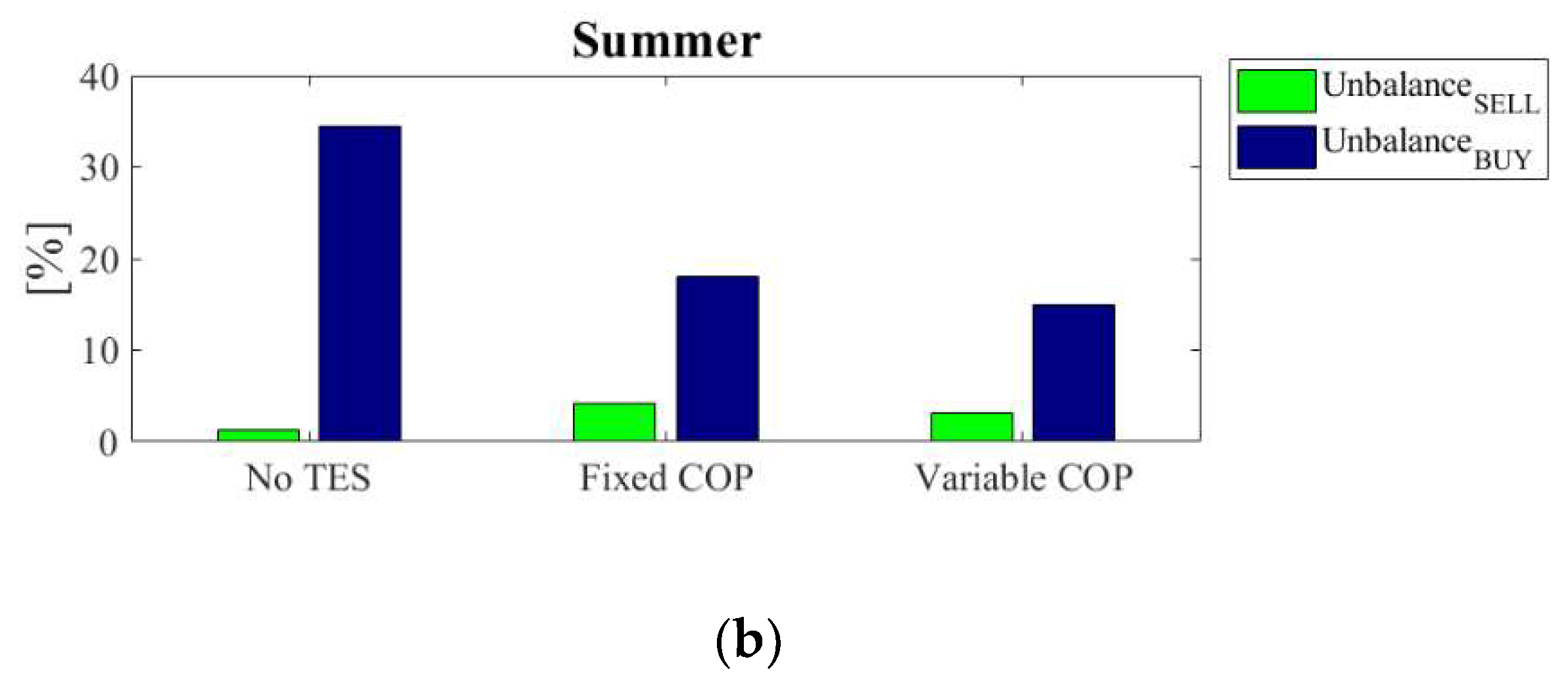
• In the winter, a strong reduction of energy unbalance (in the order of 20%) has been achieved including a TES. In the summer, despite the overall unbalanced energy exchanged with the grid is lower for the “No TES” case, a greater value in terms of unexpected energy purchased is observed.
• In the winter, the TES leads to reduce the number of HP startups while decreasing the average load factor. The load factor trend is similar in the summer, while the number of HP startups is increased for the TES cases with respect to the cases without TES.
• Benefits in the stabilization of comfort conditions have also been achieved thanks to the TES. Room temperature has more stable profiles as standard deviation gets lower by a margin of 2% to 5%.

References

1. Eurostat, Consumption of Energy, Statistics Explained Website, Data extracted in June 2017. Available online: http://ec.europa.eu/eurostat/statistics-explained/index.php/Consumption_of_energy (accessed on 1 March 2019).
2. Energy Consumption in Households. Available online: https://ec.europa.eu/eurostat/statistics-explained/index.php?title=Energy_consumption_in_households (accessed on 1 March 2019).
3. European Parliament and Council. Directive 2010/31/EU on the Energy Performance of Buildings; European Parliament and Council: Brussels, Belgium, 2010. [Google Scholar]
4. Kim, N.K.; Shim, M.H.; Won, D. Building Energy Management Strategy Using an HVAC System and Energy Storage System. Energies 2018, 11, 2690. [Google Scholar] [CrossRef]
5. Hafeez, G.; Javaid, N.; Iqbal, S.; Khan, F.A. Optimal Residential Load Scheduling Under Utility and Rooftop Photovoltaic Units. Energies 2018, 11, 611. [Google Scholar] [CrossRef]
6. Javaid, N.; Ahmed, F.; Ullah, I.; Abid, S.; Abdul, W.; Alamri, A.; Almogren, A.S. Towards Cost and Comfort Based Hybrid Optimization for Residential Load Scheduling in a Smart Grid. Energies 2017, 10, 1546. [Google Scholar] [CrossRef]
7. Aslam, S.; Iqbal, Z.; Javaid, N.; Khan, Z.A.; Aurangzeb, K.; Haider, S.I. Towards Efficient Energy Management of Smart Buildings Exploiting Heuristic Optimization with Real Time and Critical Peak Pricing Schemes. Energies 2017, 10, 2065. [Google Scholar] [CrossRef]
8. Iqbal, Z.; Javaid, N.; Mohsin, S.M.; Akber, S.M.A.; Afzal, M.K.; Ishmanov, F. Performance Analysis of Hybridization of Heuristic Techniques for Residential Load Scheduling. Energies 2018, 11, 286. [Google Scholar] [CrossRef]
9. Park, L.; Jang, Y.; Bae, H.; Lee, J.; Park, C.Y.; Cho, S. Automated Energy Scheduling Algorithms for Residential Demand Response Systems. Energies 2017, 10, 1326. [Google Scholar] [CrossRef]
10. He, M.F.; Zhang, F.X.; Huang, Y.; Chen, J.; Wang, J.; Wang, R. A distributed demand side management algorithm for smart grid. Energies 2019, 12, 426. [Google Scholar] [CrossRef]
11. Lemus, F.D.S.; Minor Popocatl, O.; Aguilar Mejia, R. Tapia Olvera, Optimal Economic Dispatch in Microgrids with Renewable Energy Sources. Energies 2019, 12, 181. [Google Scholar] [CrossRef]
12. Ruiz, G.R.; Segarra, E.L.; Bandera, C.F. Model Predictive Control Optimization via Genetic Algorithm Using a Detailed Building Energy Model. Energies 2019, 12, 34. [Google Scholar] [CrossRef]
13. Kontes, G.D.; Giannakis, G.I.; Sanchez, V.; de Augustin Chamacho, P.; Romero Amortrortu, A.; Panagiotidou, N.; Rovas, D.V.; Steiger, S.; Mutschler, C.; Gruen, G. Simulation-Based Evaluation and Optimization of Control Strategies in Buildings. Energies 2018, 11, 3376. [Google Scholar] [CrossRef]
14. Barata, F.; Igreja, J. Energy Management in Buildings with Intermittent and Limited Renewable Resources. Energies 2018, 11, 2748. [Google Scholar] [CrossRef]
15. Izawa, A.; Fripp, M. Multi-Objective Control of Air Conditioning Improves Cost, Comfort and System Energy Balance. Energies 2018, 11, 2373. [Google Scholar] [CrossRef]
16. Jin, D.; Christopher, W.; James, N.; Teja, K. Occupancy-Based HVAC Control with Short-Term Occupancy Prediction Algorithms for Energy-Efficient Buildings. Energies 2018, 11, 2427. [Google Scholar] [Green Version]
17. Serale, G.; Fiorentini, M.; Capozzoli, A.; Bernardini, D.; Bemporad, A. Model Predictive Control (MPC) for Enhancing Building and HVAC System Energy Efficiency: Problem Formulation, Applications and Opportunities. Energies 2018, 11, 631. [Google Scholar] [CrossRef]
18. Robillart, M.; Schalbart, P.; Chaplais, F.; Peuportier, B. Model reduction and model predictive control of energy-efficient buildings for electrical heating load shifting. J. Process. Control. 2018, 74, 23–34. [Google Scholar] [CrossRef]
19. Bruni, G.; Cordiner, S.; Mulone, V.; Rocco, V.; Spagnolo, F. A study on the energy management in domestic micro-grids based on Model Predictive Control strategies. Energy Convers. Manag. 2015, 102, 50–58. [Google Scholar] [CrossRef]
20. Killian, M.; Zauner, M.; Kozek, M. Comprehensive smart home energy management system using mixed-integer quadratic-programming. Appl. Energy 2018, 222, 662–672. [Google Scholar] [CrossRef]
21. D’Ettorre, F.; de Rosa, M.; Conti, P.; Schito, E.; Testi, D.; Finn, D.P. Economic assessment of flexibility offered by an optimally controlled hybrid heat pump generator: A case study for residential building. Energy Procedia 2018, 148, 1222–1229. [Google Scholar] [CrossRef]
22. di Perna, C.; Magri, G.; Giuliani, G.; Serenelli, G. Experimental assessment and dynamic analysis of a hybrid generator composed of an air source heat pump coupled with a condensing gas boiler in a residential building. Appl. Therm. Eng. 2015, 76, 86–97. [Google Scholar] [CrossRef]
23. Klein, K.; Huchtemann, K.; Müller, D. Numerical study on hybrid heat pump systems in existing buildings. Energy Build. 2014, 69, 193–201. [Google Scholar] [CrossRef]
24. Bagarella, G.; Lazzarin, R.; Noro, M. Annual simulation, energy and economic analysis of hybrid heat pump systems for residential buildings. Appl. Therm. Eng. 2016, 99, 485–494. [Google Scholar] [CrossRef]
25. D’Ettorre, F.; Conti, P.; Schito, E.; Testi, D. Model predictive control of a hybrid heat pump system and impact of the prediction horizon on cost-saving potential and optimal storage capacity. Appl. Therm. Eng. 2019, 148, 524–535. [Google Scholar] [CrossRef]
26. Mohammadi, S.; Mohammadi, A. Stochastic scenario-based model and investigating size of battery energy storage and thermal energy storage for micro-grid. Int. J. Electr. Power Energy Syst. 2014, 61, 531–546. [Google Scholar] [CrossRef]
27. Nguyen, D.T.; Le, L.B. Optimal Bidding Strategy for Microgrids Considering Renewable Energy and Building Thermal Dynamics. IEEE Trans. Smart Grid 2014, 5, 1608–1620. [Google Scholar] [CrossRef]
28. Korkas, C.D.; Baldi, S.; Michailidis, I.; Kosmatopoulos, E.B. Occupancy-based demand response and thermal comfort optimization in microgrids with renewable energy sources and energy storage. Appl. Energy 2016, 163, 93–104. [Google Scholar] [CrossRef]
29. Comodi, G.; Giantomassi, A.; Severini, M.; Squartini, S.; Ferracuti, F.; Fonti, A.; Cesarini, D.N.; Morodo, M.; Polonara, F. Multi-apartment residential microgrid with electrical and thermal storage devices: Experimental analysis and simulation of energy management strategies. Appl. Energy 2015, 137, 854–866. [Google Scholar] [CrossRef]
30. Bartolucci, L.; Cordiner, S.; Mulone, V.; Santarelli, M. Short-therm forecasting method to improve the performance of a model predictive control strategy for a residential hybrid renewable energy system. Energy 2019, 172, 997–1004. [Google Scholar] [CrossRef]
31. Gelleschus, R.; Böttiger, M.; Stange, P.; Bocklisch, T. Comparison of optimization solvers in the model predictive control of a PV-battery-heat pump system. Energy Procedia 2018, 155, 524–535. [Google Scholar] [CrossRef]
32. Bartolucci, L.; Cordiner, S.; Mulone, V.; Rocco, V.; Rossi, J.L. Renewable source penetration and microgrids: Effects of MILP–Based control strategies. Energy 2018, 152, 416–426. [Google Scholar] [CrossRef]
33. ELFOEnergy Extended Inverter, SERIE WSAN-XIN 81-171. Available online: http://portal.clivet.it/products/app.jsp# (accessed on 1 March 2019).
34. Available online: http://www.meteoam.it/ta/previsione/482/ROMA (accessed on 1 March 2019).
35. Sousa, T.; Morais, H.; Castro, R.; Vale, Z. Evaluation of different initial solution algorithms to be used in the heuristics optimization to solve the energy resources scheduling in smart grid. Appl. Soft Comput. 2016, 48, 491–506. [Google Scholar] [CrossRef]
36. Verhelst, C.; Logist, F.; Impe, J.V.; Helsen, L. Study of the optimal control problem formulation for modulating air-to-water heat pumps connected to a residential floor heating system. Energy Build. 2012, 45, 43–53. [Google Scholar] [CrossRef]
37. Available online: http://www.meteoam.it/page/verifiche-modelli (accessed on 1 March 2019).
Figure 1. Scheme of the residential hybrid renewable energy system.
Energies 12 02429 g001
Figure 2. Thermal physical model.
Energies 12 02429 g002
Figure 3. Weekly thermal load profiles for the winter and summer season.
Energies 12 02429 g003
Figure 4. Scheme of the thermal subsystem of the HRES. (a) System configuration without the TES. (b) System configuration with TES.
Energies 12 02429 g004
Figure 5. Daily value of the EER as a function of a typical temperature pattern in the summer season.
Energies 12 02429 g005
Figure 6. Cash flow for the three test cases: without TES, with TES and fixed COP, and with TES and variable COP.
Energies 12 02429 g006
Figure 7. (a) Total energy unbalance for the three cases for the winter and the summer season. (b) Energy unbalance sold and bought for the three test cases for the summer season.
Energies 12 02429 g007aEnergies 12 02429 g007b
Figure 8. Difference between real and expected (forecast) ambient temperature in the winter and the summer.
Energies 12 02429 g008
Figure 9. (a) Number of startups of the Heat Pump for the three cases in the winter and the summer. (b) Statistical Distribution of the Load Factor of the Heat Pump for the three cases in the winter and the summer.
Energies 12 02429 g009aEnergies 12 02429 g009b
Figure 10. (a) Real indoor ambient temperature for the three test cases in the winter and the summer. (b) Ambient temperature deviation from the reference temperature for the three test cases in the winter and the summer.
Energies 12 02429 g010